This is an accepted manuscript of an article published by Elsevier in Journal of Transport
Geography on May 13 2017, available at https://doi.org/10.1016/j.jtrangeo.2017.05.002 This manuscript version is made available under de CC-BY-NC-ND 4.0 license
http://creativecommons.org/licenses/by-nc-nd/4.0/ Please cite as:
Devaux, N., Dubé, J., & Apparicio, P. (2017). Anticipation and post‐construction impact of a metro extension on residential values: The case of Laval (Canada), 1995– 2013. Journal of Transport Geography, 62, 8‐19. doi:10.1016/j.jtrangeo.2017.05.002
ANTICIPATION AND POST‐CONSTRUCTION IMPACT OF THE METRO EXTENSION ON RESIDENTIAL VALUES: THE CASE OF LAVAL (CANADA), 1995‐2013. ___________________________ Abstract
The application of hedonic pricing models has a long history in estimating the externalities associated with urban infrastructure, such as public transportation. However, results accuracy crucially depends on methodological and empirical considerations such as: i) presence of spatial latent component (spatial autocorrelation); ii) temporal breaks related to different periods over which the infrastructure is built; and iii) heterogeneity of the effect along the line and stations. This paper aims to assess the impact of Montréal’s metro extension to the suburb city of Laval (announced in 1998 and started operating in 2007). A spatial difference‐in‐difference (SDID) estimator based on a repeated sales approach is used to isolate the impact of the proximity to the new infrastructure on single‐family house prices depending on the implementation phases and the stations. The results suggest that among the three new infrastructures, only one shows a positive impact of proximity after the first operation of the transit service. The study results tend to relativize the sometimes high expectations in terms of economic impacts of such a project, at least for residential properties. Keywords Hedonic Pricing Model; Public Transportation; Housing Values; Spatial difference‐in‐ differences (SDID) Estimator; Repeated Sales Approach; Spatiotemporal Analysis
1. INTRODUCTION
Derived from Ricardo and von Thünen’s seminal work, the Alonso (1964) model allows explaining the urban price gradient as a function of the distance to a central business area (McMillen, 2006). In its first version of the paper, the bid‐rent location curves explicitly introduce the importance of transportation cost has a factor that shape land prices. Transportation cost implicitly includes the possibility that urban infrastructures, such as public transport, can shape land and real estate prices. This has also been recognized previously through the work of Wingo (1961). A reduction in transportation costs through the development of new public transport infrastructure should, consequently, be translated into land and property values (Kim and Lahr, 2014). Thus, location rent can be isolated using proximity to mass transit lines or stations, depending on the type of public transportation. Yet, it must be admitted that the assessment of the expected impacts by planners and policymakers remains a complex task (Higgins and Kanaroglou, 2016). Despite abundant literature on the topic, varying results are observed between studies (Debrezion et al., 2007) ranging from negative to positive effects (Kim and Lahr, 2014).
The latent spatial components of the price determination process (Lancaster, 1966; Rosen, 1974) invalidate standard regression assumptions of independence (Anselin and Griffith, 1988; Legendre, 1993) and, by extension, conclusions drawn by empirical applications. From a methodological perspective, it is well recognized that real estate values are location dependent, which can result in spatial autocorrelation among residuals of pricing equations (Can, 1992; Dubin, 1998). Spatial autocorrelation is a central concept in empirical spatial research (Getis, 2008) and is defined as the coincidence between measures depending on location (Anselin and Bera, 1998; Lesage and Pace, 2009). It may be associated with the omission of significant spatial variables (Mcmillen, 2010) or with spatial dependence processes structuring a data generating process (Le Gallo, 2002).
Other methodological challenges emerge when trying to isolate the effect of accessibility to a mass transit (MT) system on real estate values. The impact may be heterogeneous and varies over time according to the implementation phases of the development of new MT lines, but also among the stations serving the line. For a major MT development project, the development and construction of infrastructures can be broken down into distinct implementation phases (announcement, construction, operation) during which the impacts on real estate values can fluctuate according to anticipation effects of the market. Stated otherwise, the impact measured during the planning periods can well be different from the final impact according to possible speculation or anticipation effects (Mcdonald and Osuji, 1995; Mcmillen and Mcdonald, 2004; Agostini and Palmucci, 2008; Atkinson‐Palombo, 2010). While a global assessment of the effect is often realized for the whole transportation system once in operation, station effects are also likely to generate localized premium distinctions (Hess
and Almeida, 2007) due to station characteristics, services quality or landscaping and urban development choices.
The paper aims to assess the impact of the extension of Montreal’s subway on the (suburban) island of Laval (on the north side) using 5,422 repeated (pairs of) transactions collected between 1995 and 2013. Repeated‐sales approach (Bailey et al., 1963; Case and Shiller, 1987) is used and matched with a spatial difference‐in‐difference model (SDID) (Dubé et al., 2014) to deal with possible spatial omitted variables and control for spatial spillovers over transaction prices. For comparison purposes, two model specifications are estimated. The first assesses the premium associated with each project implementation phase from a global perspective (all stations combined) while the second breaks down this periodic effect for each new station. Additional statistical tests for homogeneity and cumulative significance effect over the implementation phases are performed. Moreover, the impact is not homogenous along the transport line and implementation periods, with only positive significant effect being estimated for one of the three stations observed after the first operation.
The paper is divided into five sections. The first section is dedicated to literature review presenting previous empirical studies and paying special attention to the variation of study results depending on the project implementation phases and contextual factors. The second section covers the proposed modeling approach. The third section presents the data used to estimate the model, while the fourth section presents the estimation results. The last section covers a discussion and a conclusion closes the paper. 2. LITERATURE REVIEW
The bid‐rent theory, first introduced by (Alonso, 1964; Mills, 1969; Muth, 1969), suggests that land prices are a decreasing function of distance to the center (or central business district ‐ CBD). According to the complex structure of actual cities, theory needs to be considered according to realities such as urban sprawl and polycentric forms (Heikkila, 1989). In this context, the development of the transportation infrastructures contributes to supplant the notion of physical proximity to the benefit of accessibility and modifies the distribution of socio‐economic profiles across urban space (Glaeser et al., 2008). According to Burgess (2008), an increased mobility acts as a catalyst of change in a city and land values are “one of the most sensitive indexes of mobility” (idem: 344) explaining the consideration for hedonic pricing modeling using property values to isolate the impact of mobility through proxies such as distance to mass transit system and infrastructure. As such, high expectations are associated with mass transit systems in terms of urban and economic developments (Dittmar and Ohland, 2004; Hess and Lombardi, 2004; Landis et al., 1994; Calthorpe, 1993). Since the early work of Dewees (1976) and Bajic (1983), our capacity to predict the impact of those development policies is still limited (Handy, 2005) and the extensive literature reflects great results variability due to spatial and temporal considerations.
Regarding spatial consideration, each station is different and can produce a distinctive impact (Hess and Almeida, 2007). In fact, from an urban development perspective, each station can be perceived as a singular infrastructure with service, structural and landscaping particularities. The premium measured may not be homogenous over the whole transportation system’s line and may vary due to station characteristics effects. One source of station‐related result variation could be associated with the complementarity between transportation modes (Voith, 1993; So et al., 1997; Ryan, 2005), and other transportation modes may even impact the premium due to substitution effects (Ryan, 1999; Baum‐Snow et al., 2005).
As exposed by Bowes and Ihlanfeldt (2001) the presence of parking facilities positively affects the sales prices. By studying Hamburg's transit system, Brandt and Maennig (2012) state that subterranean stations significantly increase the impact on condominium prices. The location of the station has also been noted as a factor influencing the premium. According to Cervero (2006) and Mulley et al. (2016), the most important premium is for residential and commercial values near downtown stations, with the impact varying among the MT system, with the higher effect related to commuter rail services (Debrezion et al., 2007). Of course, the effect may not be linear over space (Chen et al., 1997), but follow an inverse U‐shape. Empirical works noted that the effect of proximity may be lowered by negative externality predominance such as noise, pollution or criminality (Bajic, 1983; Diaz and Mclean, 1999; Bowes and Ihlanfeldt, 2001).
An additional challenge related to evaluating the impact of such infrastructures relies on the fact that the development of a new MT system takes a considerable amount of time and money to be built. Agostini and Palmucci (2008) suggested that the impact can be decomposed into three distinct phases: announcement period; construction period; and operation period. The announcement period refers to the moment the project is publicized. During this period a speculation effect may be observed indicating a first market response (anticipation) to an MT system development. The second phase, the construction period, marks the realization of the project. At that time the location of the future stations is concretely observed by the public, where the anticipation effect can be exacerbated. McMillen and McDonald (2004) considered the Chicago transit system and pointed out that house prices were affected even before the stations were built but after the project plans were known. Bae et al. (2003) also identified anticipation effects for the construction of a subway line in Seoul. Knaap et al. (2001) and Atkinson‐Palombo (2010) identified capitalisation benefits from the time the project was publicly known. Studying Santiago’s metro system, Agostini and Palmucci (2008) have noted that the average apartment price rises after the project has been announced, and that there is smaller, but positive and significant, impact after the identification of the station location. On the opposite side, Yan et al. (2012) did not
observe any anticipation effect of the project proximity on home prices before the rail system began operation in Charlotte (North Carolina).
After the MT comes into operation, the maturity of the service is another plausible source of impact variation. While a number of studies note a positive impact of fully developed light rail systems on real estate values (Cervero and Duncan, 2002; Weinstein et al., 2002), Gatzlaff and Smith (1993) did not find any relationship for a semi‐ developed rail system. Mohammad et al. (2013) illustrate those conclusions by citing the example of the Metropolitan Atlanta Rapid Transit rail system (MARTA) whose impact was first studied 10 years after its initial operation by Nelson and McCleskey (1989). The authors only found a minimal effect while, a few years later Bowes and Ihlanfeldt (2001) identified positive and negative effects depending on the location. On the opposite side, Cervero and Landis (1997) assessed the impact of the Bay Area Rapid Transit (BART) system during its first 20 years of operation. The results for the fully developed service are consistent with those previously obtained after the first operation (Dyett et al., 1979).
Considering spatial and temporal dimensions, the decomposition and isolation of a proximity effect of a new transportation station per project implementation phase and station implies devising an appropriate econometric model. 3. METHODOLOGY AND RESEARCH STRATEGY
Hedonic theory and price function is one of the most used methodologies to break down the value of a complex good into its characteristics’ implicit prices (Rosen, 1974). The approach is based on revealed preferences: actual sale price reflects an equilibrium reached where both agents (buyer and seller) agree on a given amount (pay and receive) for a given bundle of goods according to the composition of the bundle. Widely documented in the urban and real estate literature, the hedonic pricing model therefore allows modeling the price of a real estate good as a function of its intrinsic and extrinsic attributes. The former relate to the elements describing the property sold while the latter are associated with environmental or location factors.
The log‐linear functional form is described as one of the most used and best linear specifications (Cropper, 1988; Rasmussen, 1990, Dubé et al., 2013)1. The hedonic pricing model expresses the sale price (in logarithmic transformation) of a property i at time , stacked in a vector of dimension 1 , where corresponds to the total number of observations ( ∑ ), as a function of the amenities of the goods, intrinsic and extrinsic, stacked in matrices and , respectively of sizes and , where is the total number of intrinsic amenities and is the total number
1 The proper functional form has been tested using a Box‐Cox transformation on the sale and resale prices.
of extrinsic amenities. To account for the fact that prices are usually expressed in nominal terms, a set of temporal dummy variables, stacked in a matrix of dimension N 1 , is usually added to the model specification. Finally, it is current to explicitly account for a spatial spillover effect in real estate markets by using a spatial autoregressive specification based on the spatial lag of the dependent variable (Equation 1).
(1)
Where is a row‐standardized spatial weights matrix, of dimension , and the resulting spatial variable, , expresses the mean sale price of properties in the direct vicinity. The vectors of parameters, , , and are, respectively, of dimension 1 1 , 1 and 1 , with , and measuring the implicit prices of the amenities, while the parameters and are scalars measuring, respectively, the constant term and the strength of the transaction price's spatial dependence (Lesage and Pace, 2009).
The analysis of the impact of an “exogenous” change in extrinsic amenities can be explored using a difference‐in‐differences (DID) specification by identifying the moment where change occurs over time. In the case of a new MT system, the change can be break down into four (4) distinct phases. Keeping the pre‐announcement period as reference, each ∗ period is defined by: announcement ∗; construction ∗; and the operation ∗ (Equation 2). ∗ 1 ∗ ⩽ ⩽ ∗ 0 ∗ 1 ∗ ⩽ ⩽ ∗ 0 ∗ 1 ⩾ ∗ 0 (2) Multiplying these indicator variables by the appropriate extrinsic amenities returns the spatial DID (SDID) estimator.2
To simplify the presentation, let's stack these dummy variables in a matrix, , that identifies the moment of the sale during the phases of the project. A Hadamard product, ⨀, is used as a term‐by‐term multiplication isolating the effect of the change on the extrinsic amenities’ matrix, where the three 3 vectors of parameters, , are all of dimension ∗ 1 , where ∗ is the total number of extrinsic amenities changing over time and assume an homogenous effect within all stations considered.
2 Considering that spatial autocorrelation rises by dependency process between sale prices, a spatial difference‐in‐difference (SDID) (Dubé et al., 2014) is estimated controling for spatial spillovers.
Multiplying the matrix of temporal indicators to the extrinsic amenities that change over time returns the DID estimator (Equation 3)
⨀ ∗ (3)
Where ∗ is the matrix of extrinsic amenities that change over time, of dimension ∗ .
Of course, and as previously mentioned in the literature review, the premium measured for proximity to a new transportation station may differ among stations. In order to assess a possible distinctive effect for each new station, a new variable (vector), , is included in the specification to isolate the closest station from the new MT line. The matrix is composed by S different vector of dimension 1 , where a given vector, ,
⨀ ⨀ ∗
(4)
Where the vector of parameter are all of dimension ∗ 1 .
The SDID estimator can be estimated using a price equation. However, it can also be estimated using a reduced form based on the repeated‐sales (RS) approach. The RS approach is a well‐known method to develop a price index of the evolution of real estate values (Bailey et al., 1963). It also allows to adequately control for latent spatial structure constant over time (Dubé et al., 2011; Dubé et al., 2013). Moreover, the SDID estimator using the RS approach has the advantage of being exempt from problems related to the functional form (Mcmillen, 2010) and omitted variables (Dubé et al., 2014). Furthermore, as mentioned by Kim and Lahr (2014) and based on the work of Wang and Zorn (1997), the use of an RS approach allows avoiding the use of critical property characteristics.
However, the DID and SDID estimator relies on three assumptions (Dubé et al., 2014). First, it assumes that the coefficients are constant over time (Case and Shiller, 1987; Case and Shiller, 1989), meaning that preferences remain unchanged. Second, it considers, if no information is available to describe changes in amenities, that intrinsic amenities are constant over time (Dubé et al., 2011). Finally, it assumes that the frequency of the sale of a good follows a random process suggesting that no characteristic affects the sale frequency of a property (Gatzlaff and Haurin, 1997; Gatzlaff and Haurin, 1998).
Since repeated transactions are only a fraction of total transactions, sample size is reduced ( ). Individual observations consist of houses first sold in time and with the resale in time . The SDID estimator is obtained by using the first difference from the hedonic pricing model according to the moment of the sale.
Depending on the specification used (equations 3 or 4), the SDID based on repeated sales approach (using a first difference equation) returns a different and reduced form (equations 5 or 6, respectively). ∆ ∆ ∆ ∆ ⨀ ∗ (5) ∆ ∆ ∆ ∆ ⨀ ⨀ ∗ (6)
Where ∆ is the price growth within two transactions (sales and resales3 ‐ ∆ log ⁄ ). Since intrinsic amenities are assumed to be unchanged between the sale and resale periods, their effect is cancelled by the first difference (∆ ). Moreover, the change in extrinsic amenities is captured through the multiplicative (DID) term, resulting also in cancelling the vector of extrinsic amenities (∆ ). The matrix ∆ corresponds to the difference (variation) in log of sale price (and approximation of price growth) and is of dimension 1 , where is the total number of pairs of transactions.4 Similarly, ∆ corresponds to the variation of the autoregressive parameter (spillover effect) and is of dimension .
The elements of the matrix ∆ , indicating the month of the sale
1 and resale 1 , can thus take a value of 1, 0 or ‐1. By the same token, the exogenous changes in the period of the implementation process are captured by the matrix ∆ of dimension . The elements of the matrix take the value of 1 during the first sale 1 as well as at the moment of the resale
1 . Thus, as for the ∆ matrix, the elements of the matrix ∆ can take a value of 1 (a change occurs in the resale period), a value of 0 (no change occurs between moment of sale and resale), or a value of ‐1 (a change occurs during the sale period). The general elements of the matrix ⨀ , of dimension , take a value returning the distance to the closest station for transactions occurring at least twice. Finally, is a vector of error terms of dimension 1 and assumed independent and identically distributed (iid). 4. CASE STUDY AND DATA 4.1 The Laval metro extension project
3 Where ∆ log log , or equivalently ∆ log ⁄ ), and where the dependent variable expresses the logarithmic transformation of the final sale price ( log ),.
4 Since repeated transactions (couples of sale and resale) are only a fraction of the total transactions, we should have << .
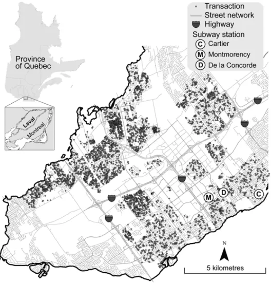
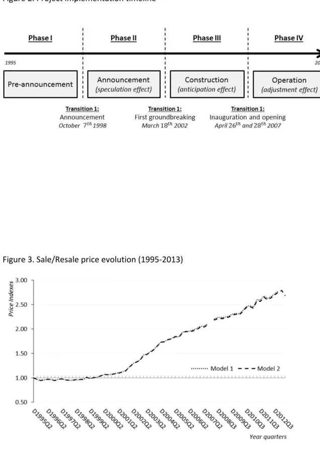
The city of Laval has a population of 369 000 inhabitants, located in the northern suburbs of Montréal and is therefore part of the greater metropolitan area in the province of Québec. For the urban agglomeration of Montréal, over 51% of the population is living in Laval but nearly 53% work on Montréal Island mainly in the service sector (82%).5 The general configuration of the whole city region is distinguished by the presence of the river physically isolating Laval and Montreal islands from the North and South shores (Figure 1). INSERT FIGURE 1 HERE: Map of Laval Before the extension of Montreal’s subway (orange line) to Laval, bridges and commuter trains allowed access to Montreal Island, and no other subway lines were available in Laval. According to the policy makers, the project of the extension of the actual subway line aimed to decongest roads, increase residents' quality of life, while being part of a “sustainable development” approach from an environmental perspective. The new transportation stations were first announced by the Parti Québécois, a provincial political party in power at the time, in October 1998, for an approximate cost of $179M. Originally the project was designed for a single station but two additional stations were added. In 2001 corrections were made to the original project so that the planned costs were subsequently re‐evaluated at $379M. The total length of the orange line is now about thirty kilometers and has 31 stations, with the new section being slightly over 5 km in length (Figure 2). INSERT FIGURE 2 HERE Project timeline The first ground was broken in March of 2002. After the election of the Parti Libéral du Québec, another provincial political party, in 2003 and with the beginnings of the construction, the cost continued to rise, to reach a total of $803.6M. From the total cost, $785.3M was reimbursed by the governments (provincial and federal) and $18.3M by the Agence Métropolitaine de Transport (AMT). However, after the completion and first operation of the subway in April 2007, some confusion remains regarding the total project costs.
The closest station to Montréal, Cartier station, is an intermodal facility with a connection to the bus system and 465 parking spaces. A part of the station is dedicated to small shops. The second station, De la Concorde station, is also an intermodal facility, but with a connection to the commuter train. Finally, the Montmorency station also features a link to bus lines and 1,357 indoor and outdoor parking spaces, but it is distinguished from other stations, being the terminus of the metro line, while most of the buildings surrounding the station are devoted to commercial activities. In all cases,
the alternative transportation modes were available prior to the metro extension and before the first observed property transaction of our dataset. Their respective effect is then cancelled by the DID estimator (no difference between the sale and resale). However, the multimodal nature of the new subway facility could explain individual station effect variations. Landscaping around the stations was done, to include gardens, and could also explain station‐related effect variations. Since the end of the work, new expansion projects are regularly planned but not yet underway. 4.2 Property transaction data
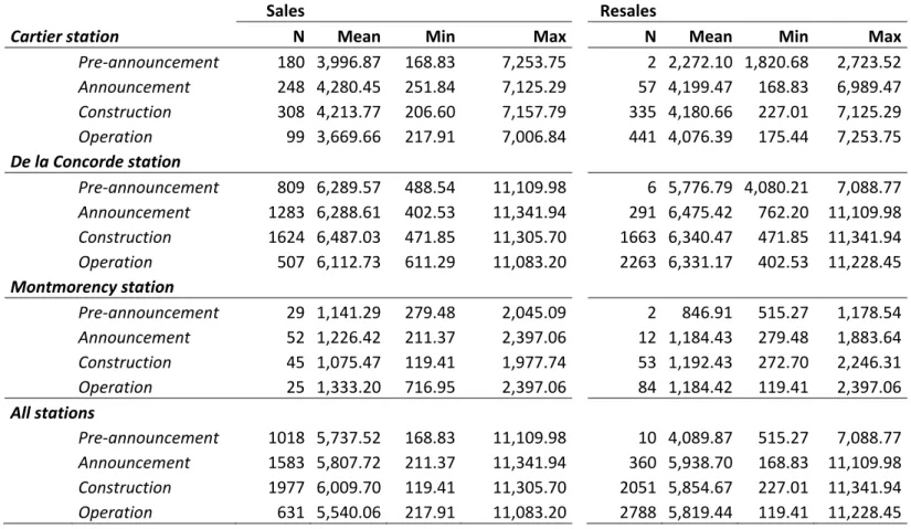
The transactions data are obtained from the Greater Montréal Real Estate Board (GMREB) and originally consist of 22,160 residential property ( ) transactions between 1995 and 2013 in the city of Laval. Each observation contains information on the transaction price and addresses allowing to geocode each property at its exact coordinates using a geographic information system (GIS). From the total number of transactions, the observations with incomplete data or selling price information are rejected. The repeated sales approach uses only transactions appearing at least twice, and a maximum of 6 times, reducing the sample size to 5,244 pairs of transactions. To avoid possible bias caused by quick renovations with the intention of reselling the property (flip), property sales and resales within a minimum interval of 6 six months have been discard. In the end, the sample consists of 5,209 pairs of transactions (sale and resale ‐ ) used for the repeated sale hedonic modeling. The distribution of sales and resales per period is presented in Table 1. INSERT TABLES 1 AND 2 HERE Distribution of the number of transactions per year and phases
The mean sale price is $137,776 (CAD) while the mean resale price is $209,847. According to the distribution of the sales and resales for each year (Table 2), the total number of sales is relatively limited during the first years of the dataset corresponding to the pre‐announcement period. This number increases slightly during the announcement period and grows more markedly for the subsequent periods (construction and operation phases). A total of 631 sales and 2,788 resales experienced the new transportation service by being observed after April 2007 (operation phase). Similarly, respectively 1,977 and 2,051 sales and resales are observed during the construction period while 1,583 sales and 360 resales are recorded between the announcement and the beginning of the construction work (Table 2).
By using the exact location of the properties, the Euclidean distance ( ) to the closest metro station is computed, and the inverse distance (1⁄ ) is used as an independent
variable.6 Considering the first transactions (sales), the mean distance is higher for properties sold during the announcement phase (14,242 m.), while the lowest distance is observed during the construction phase (258 m.). Considering the second transactions (resales), the same mean distance, maximum and minimum mean distances, are respectively observed during the construction phase and after the first operation of the service (Table 3). INSERT TABLE 3 Distance to the nearest railway station 5. RESULTS 5.1 A global perspective As previously mentioned, two categories of models are estimated: i) one that assumes a homogenous effect within stations among the different periods (Equation 5); and ii) one that allows different effect for each stations among the different periods (Equation 6). The first specification allows for temporal decomposition of the proximity impact to the stations according to the period of the implementation process, while the second allows for a temporal decomposition of the proximity impact on house prices as well as for spatial decomposition according to the station. Both models' specifications are estimated using a GLS estimation and a spatial two‐stage generalized least squares (GS2SLS)7 accounting for possible heteroscedasticity,8 while the latest model also controls for a spillover effect between properties.
The SDID transformation simplifies the model specification but has the particularity of eliminating the constant term, affecting the interpretation of the statistic (Wooldridge, 2012). The model’s performance is then assessed using the Akaike Information Criterion (AIC) and the Bayesian Information Criterion (BIC).
6 The Euclidean distance ( ) is computed using: . Where and represent the coordinates of the observations i and j.
7 Prior to the GS2SLS models, maximum likelihood estimations are performed showing evidence of heteroscedasticity likely to affect coefficients' variance precision. The GS2SLS estimation model is used in order to address this issue. Such an estimator requires instruments corresponding to a linear combination of the matrices , , , etc., where is a row‐normalized spatial weights matrix and the different powers of (see Kelejian and Prucha, 1998 and 1999; Lee, 2003). For the estimation process, we have chosen to fix 2. We have performed different tests using higher power (3 and 4), but the results appear to be similar. The choice of 2 appears to be appropriate based on Monte Carlo simulations according to Drukker et al. (2013). The model was estimated using Stata.
8 As described in the methodology section, the spatial weight matrix is restricted to the transactions occurring during the same period and is specified using an inverse distance function. According to LeSage and Pace (2014), the choice of the distance function has no impact on the modeling estimations. Different weights matrix functions (negative exponential of binary) were tested. The results remain robust for the different specifications.
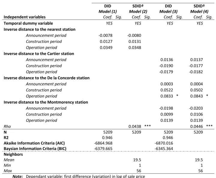
Keeping the first quarter of 1995 as the reference period, the price index fluctuations of the sale/resale properties over the considered period show that market trends experience a 102% (Model 4) to 107% (Model 1) increase of the price between sale and resale depending on the model specification (Figure 3).9 INSERT FIGURE 3 HERE Price index fluctuation Assuming a homogenous effect for all the stations, and keeping the pre‐announcement period as reference, no significant effect of proximity to the new stations is observed. A statistical test is performed to evaluate the global impact ( 0) and suggests no significant impact (Table 5a). Stated otherwise, the global property values are not impacted by the new transit infrastructure. Thus, this issue raises the question of the uncertainty of the effect over time and could challenge some expectations in terms of economic benefits in the long term. INSERT TABLE 4 HERE Estimation results
INSERT TABLES 5A AND 5B HERE Statistical test results INSERT FIGURE 5 HERE Proximity effect in function of distance 5.2 A station‐oriented perspective
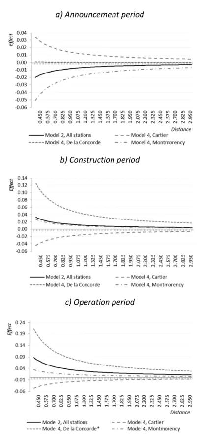
According to Model 3 and Model 4, significant heterogeneity between the stations is detected: only De la Concorde station reveals significant impact on house price changes, with a coefficient of 0.0833 (model 3) and 0.843 (model 4) during the operation period (Table 4 and Figure 4). Moreover, the assumption of homogenous impact can be formally addressed using a formal statistical test within stations and periods (
). The results show no significant distinction within the station during the announcement and construction periods (Table 5b). However, the test performed on the third phase reveals a significant difference for the impact among the stations (Table 6b), underlining a homogenous effect of proximity on house prices. 9 A similar index was built for transactions in the northern section, as well as for the southern section of the city, and no significant difference in trends was noted.
Another series of tests is also computed to assess whether the global impact (sum of the three periods) per station is significant ( 0 – Table 6b). None of
the announcement periods ( 0) nor construction period (
0) presents significant results. Again, no evidence of a significant effect is noted for the last phase ( 0), which leads to a conclusion assuming a homogenous effect. 5.3 Calculating the impact on house prices The spatial specification used (SDID) allows capturing and measuring the effect of spatial spillovers. The spillover effect needs to be accounted for when calculating the marginal effect since it acts as a chain reaction influencing prices of other houses sold at the same time period. Thus, the interpretation of the regression parameters can no longer be interpreted as the direct marginal effect on property prices unless the autoregressive parameter, ρ, is non‐significant (Dubé et al., 2014).
With the standard GLS model, the marginal effect computation is straightforward and refers to the proportion of change in the dependent variable for one unit change in the independent variable (Equation 7). However, using a spatial specification this marginal effect also includes the induced effect of a change in all the neighboring dependent variables, . As presented by LeSage and Pace (2009), the total marginal effect in a spatial context is then obtained by the following derivative (Equation 8). (7) (8)
In the case of the present analysis, considering the fact that the ρ coefficient is significant in both specifications, the marginal effect computation should be based on Equation 8. Moreover, since the impact varies according to the distance to the nearest station, the marginal effect needed to be decomposed to account for both effects: distance and spillover.
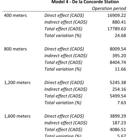
For simplicity's sake, only the last specification, the non‐homogenous effect within stations and periods, is discussed (De la Concorde station during the operation period). Regarding the estimation results, marginal effects for different distances, varying between 400 to 1,600 meters, are reported for the De la Concorde station according to the significant results only (Table 6). The full decomposition of the direct and total marginal effect, based on the decomposition of the spatial multiplier (Steimetz, 2010) is reported in Figure 4.
INSERT TABLE 6 HERE Effect of distance in dollars ($)
For the operation period, at a distance of 400m the direct marginal effect suggests a price increase of CAD$16,909, while the total marginal effect suggests a CAD$17,789 price increase, corresponding to a 24.7% price increase. The difference between both effects represents the indirect marginal effect, measuring the impact of the spatial spillover effect.
The same decomposition can be done for other distances, while the impact reduces with higher distances (Table 6). For example, increasing distance by 400 meters lowers the total marginal impact on house prices to CAD$8,405 at 800 meters (a 11.66% price variation), to CAD$5,499 at 1,200 meters (a 7,6% price variation) and to CAD$4,086 at 1,600 meters (a 5.7% price variation). Figure 5 illustrates the non‐linear total effects. Overall, the estimated impact of the De la Concorde’s station proximity is higher when the spatial multiplier is considered and consequently influences study results. 6. DISCUSSION The results show a limited effect, in space and time, for proximity to the metro stations, questioning certain expectations in terms of economics impacts, at least in the single‐ family market. Thus, in comparison to previous studies (Bae et al., 2003; Mcmillen and Mcdonald, 2004; Gibbons and Machin, 2008) no anticipation effect is measured. Global measures show no significant effect, neither does the decomposition of the effect per period. Pushing this decomposition further, only one station shows evidence of positive proximity effect (the De la Concorde station). According to these results, not only is the effect of proximity heterogeneous among the different implementation phases, but it also presents differences among stations. Aggregating the effect in a single and homogenous coefficient hides the impact measured for the De la Concorde station. Moreover, the SDID specification allows considering spatial spillovers in the total measured effect, suggesting a greater effect than suggested by coefficients.
A number of reasons could explain these variations between stations, such as contextual factors, station characteristics, but also the socio‐economic status of the surrounding neighborhoods. The premium measured is the equilibrium between positive and negative amenities evaluated by both sellers and buyers. By being the terminus of the line and located in a mainly commercial sector, with a highway and a college nearby, the coefficient associated with the Montmorency station may be affected by negative externalities overbalancing positive advantages of public transportation service proximity. However, it should be noted that the Montmorency station presents a small number of properties nearby, which can explain the absence of significant results. Even if not significant, the effect of the Montmorency station is negative during the
announcement period and turns positive at the moment of the construction (Figure 4). The Cartier Station is located closer to a bridge connecting Laval to Montréal as compared to the other stations. A positive impact of the infrastructure could be cancelled by the density of daily commuters traveling this route, the bridge acting as a funnel. The car may also be a good alternative for residents of this area. It should be noted that, even if not significant, the impact of the station is positive during the announcement period and becomes negative at the moment of construction (Figure 4). Finally, the positive effect associated with the De la Concorde Station may be due to its multimodal connection to the suburban train or the green landscaping developments. It also appears to be the station with the highest density of neighboring residential properties.
According to these results, a global approach (all stations combined) that measures the impact reduces the significance of the results, and lowers the effect related to a given station within the impact of other stations that show no significant results. By decomposing the effect of the new infrastructure per period and stations, the estimation outlined differentiated effects over space and time. In fact, in an aggregated perspective, the post operation impact of De la Concorde station is hidden. A better understanding of these effects could help to better assess the economic impacts of such projects and formulate more realistic expectations according to contextual variations.
Overall, even if the analysis is limited to single‐family properties, the economic impacts of the transportation system remain subtle and doubts remain about the whole project's profitability at this time. The location choice of the new stations as well as the general structure of the transit system (metro line and multimodal connections) could be determining factors. The train enjoys a positive reputation, making it the preferred choice when the time comes to develop a new public transport network. However, other alternatives, such as the bus, can be just as effective at lower costs if properly designed (Hensher, 2016).
7. CONCLUSION
The impact of a rail transit system development on property values has been well studied, generally leading to a positive effect on property transaction prices. However, the construction of such infrastructures is part of a long process and may fluctuate over space and time. The analysis aimed at decomposing the effect of proximity to a metro line extension per project implementation phase (announcement, construction, operation) and new stations according to spatial and temporal decomposition. Considering the extension of the Montréal subway to the city of Laval, a spatial difference‐in‐differences (SDID) approach based on a repeated‐sales (RS) approach is applied using 5,209 pairs of transactions collected between 1995 and 2013 on single‐ family property values. The results highlighted the complexity of the assessment of a transportation service's impact on real estate values depending on temporal and spatial considerations.
From a global perspective (all stations combined), no significant effect is observed, neither after the announcement of the project nor during the construction period. No effect of the transportation service on property values is found. The decomposition of the effect over the different stations shows non‐homogenous effects over space. Results suggest that positive impact appears to be localized around a single station (De la Concorde station) during the operation period. From a methodological perspective, the SDID estimator allows considering spillover effect in the computation for a larger total effect.
Overall, the empirical application presented an innovative modeling approach to decompose the effect of a new metro infrastructure to answer some critics suggesting a lack of spatial (Hess and Almeida, 2007) and temporal (Yan et al., 2012) decomposition in such analyses. Interestingly, the observed effect is localized around a station served by a commuter train with the most dense population surrounded by residential properties. Thus, the results confirm that effects can be related to the location of individual stations as well as to the timing related to the construction of the infrastructure. However, this economic impact is limited, since it relies only on single‐ family properties. There is a strong probability that the implementation of such infrastructure may be more capitalized through commercial properties, moreover accounting for the fact that the Montmorency station is mainly surrounded by commercial buildings.
REFERENCES Agostini, C. A. & Palmucci, G. A. 2008. The anticipated capitalisation effect of a new metro line on housing prices. Fiscal Studies, 29, 233‐256. Alonso, W. 1964. Location and land use. Toward a general theory of land rent, Cambridge, MA, Harvard University Press. Anselin, L. & Bera, A. K. 1998. Spatial dependence in linear regression models with an introduction to spatial econometrics. Statistics Textbooks and Monographs, 155, 237‐290. Anselin, L. & Griffith, D. A. 1988. Do spatial effecfs really matter in regression analysis? Papers in Regional Science, 65, 11‐34. Atkinson‐Palombo, C. 2010. Comparing the capitalisation benefits of light‐rail transit and overlay zoning for single‐family houses and condos by neighbourhood type in metropolitan Phoenix, Arizona. Urban studies. Bae, C.‐H. C., Jun, M.‐J. & Park, H. 2003. The impact of Seoul's subway Line 5 on residential property values. Transport policy, 10, 85‐94. Bailey, M. J., Muth, R. F. & Nourse, H. O. 1963. A regression method for real estate price index construction. Journal of the American Statistical Association, 58, 933‐942. Bajic, V. 1983. The effects of a new subway line on housing prices in metropolitan Toronto. Urban Studies, 20, 147‐158. Baum‐Snow, N., Kahn, M. E. & Voith, R. 2005. Effects of Urban Rail Transit Expansions: Evidence from Sixteen Cities, 1970‐2000 [with Comment]. Brookings‐Wharton Papers on Urban Affairs, 147‐206. Bowes, D. R. & Ihlanfeldt, K. R. 2001. Identifying the impacts of rail transit stations on residential property values. Journal of Urban Economics, 50, 1‐25. Brandt, S. & Maennig, W. 2012. The impact of rail access on condominium prices in Hamburg. Transportation, 39, 997‐1017. Burgess, E. W. 2008. The growth of the city: an introduction to a research project, Springer. Can, A. 1992. Specification and estimation of hedonic housing price models. Regional science and urban economics, 22, 453‐474. Case, K. E. & Shiller, R. J. 1987. Prices of single family homes since 1970: New indexes for four cities. National Bureau of Economic Research Cambridge, Mass., USA. Case, K. E. & Shiller, R. J. 1989. The Efficiency of the Market for Single‐Family Homes. The American Economic Review, 125‐137. Cervero, R. 2006. Effects of light and commuter rail transit on land prices: experiences in San Diego County. University of California Transportation Center. Cervero, R. & Duncan, M. 2002. Benefits of proximity to rail on housing markets: Experiences in Santa Clara County. Journal of Public Transportation, 5. Cervero, R. & Landis, J. 1997. Twenty years of the Bay Area Rapid Transit system: Land use and development impacts. Transportation Research Part A: Policy and Practice, 31, 309‐333. Chen, H., Rufolo, A. & Dueker, K. J. 1997. Measuring the impact of light rail systems on single family home values: a hedonic approach with GIS application. Center for
Urban Studies College of Urban and Public Affairs Portland State University: Available from: http://www. upa. pdx. edu/CUS. Cropper, M. L., Deck, L. B. & Mcconnell, K. E. 1988. On the choice of funtional form for hedonic price functions. The Review of Economics and Statistics, 668‐675. Debrezion, G., Pels, E. & Rietveld, P. 2007. The Impact of Railway Stations on Residential and Commercial Property Value: A Meta‐analysis. Journal of Real Estate Finance & Economics, 35, 161‐180. Dewees, D. N. 1976. The effect of a subway on residential property values in Toronto. Journal of Urban Economics, 3, 357‐369. Diaz, R. B. & Mclean, V. Impacts of rail transit on property values. American Public Transit Association Rapid Transit Conference Proceedings, 1999. Drukker, D. M., Prucha, I. R. & Raciborski, R. 2013. Maximum likelihood and generalized spatial two‐stage least‐squares estimators for a spatial‐autoregressive model with spatial‐autoregressive disturbances. The Stata journal, 13, 221‐241. Dubé, J., Des Rosiers, F., Thériault, M. & Dib, P. 2011. Economic impact of a supply change in mass transit in urban areas: A Canadian example. Transportation Research Part A: Policy and Practice, 45, 46‐62. Dubé, J., Legros, D., Thériault, M. & Des Rosiers, F. 2014. A spatial Difference‐in‐ Differences estimator to evaluate the effect of change in public mass transit systems on house prices. Transportation Research Part B: Methodological, 64, 24‐40. Dubé, J., Thériault, M. & Des Rosiers, F. 2013. Commuter rail accessibility and house values: The case of the Montreal South Shore, Canada, 1992–2009. Transportation Research Part A: Policy and Practice, 54, 49‐66. Dubin, R. A. 1998. Predicting house prices using multiple listings data. The Journal of Real Estate Finance and Economics, 17, 35‐59. Dyett, M. V., Dombusch, D., Fajans, M., Falcke, C., Gussman, V. & Merchant, J. 1979. Land use and urban development impacts of BART: final report, US Dept. of Transportation. Gatzlaff, D. H. & Haurin, D. R. 1997. Sample selection bias and repeat‐sales index estimates. The Journal of Real Estate Finance and Economics, 14, 33‐50. Gatzlaff, D. H. & Haurin, D. R. 1998. Sample Selection and Biases in Local House Value Indices. Journal of Urban Economics, 43, 199‐222. Gatzlaff, D. H. & Smith, M. T. 1993. The impact of the Miami Metrorail on the value of residences near station locations. Land Economics, 54‐66. Getis, A. 2008. A history of the concept of spatial autocorrelation: a geographer's perspective. Geographical Analysis, 40, 297‐309. Gibbons, S. & Machin, S. 2008. Valuing school quality, better transport, and lower crime: evidence from house prices. Oxford Review of Economic Policy, 24, 99‐119. Glaeser, E. L., Kahn, M. E. & Rappaport, J. 2008. Why do the poor live in cities? The role of public transportation. Journal of urban Economics, 63, 1‐24. Handy, S. 2005. Smart growth and the transportation‐land use connection: What does the research tell us? International Regional Science Review, 28, 146‐167.
Heikkila, E., Gordon, P., Kim, J. I., Peiser, R. B., Richardson, H. W. & Dale‐Johnson, D. 1989. What happened to the CBD‐distance gradient?: land values in a policentric city. Environment and planning A, 21, 221‐232. Hensher, D. A. 2016. Why is Light Rail Starting to Dominate Bus Rapid Transit Yet Again? Transport Reviews, 36, 289‐292. Hess, D. B. & Almeida, T. M. 2007. Impact of proximity to light rail rapid transit on station‐area property values in Buffalo, New York. Urban Studies, 44, 1041‐1068. Higgins, C. D. & Kanaroglou, P. S. 2016. A latent class method for classifying and evaluating the performance of station area transit‐oriented development in the Toronto region. Journal of Transport Geography, 52, 61‐72. Knaap, G. J., Ding, C. & Hopkins, L. D. 2001. Do plans matter? The effects of light rail plans on land values in station areas. Journal of Planning Education and Research, 21, 32‐39. Lancaster, K. J. 1966. A new approach to consumer theory. Journal of Political Economy, 74, 132‐157. Le Gallo, J. 2002. Économétrie spatiale : l'autocorrélation spatiale dans les modèles de régression linéaire. Economie et Prevision, 155, 139‐157. Legendre, P. 1993. Spatial autocorrelation: trouble or new paradigm? Ecology, 74, 1659‐ 1673. Lesage, J. & Pace, K. 2009. Introduction to spatial econometrics, Boca Raton London New‐York, CRC press. Mcdonald, J. F. & Osuji, C. I. 1995. The effect of anticipated transportation improvement on residential land values. Regional science and urban economics, 25, 261‐278. Mcmillen, D. P. 2010. Issues in spatial data analysis. Journal of Regional Science, 50, 119‐ 141. Mcmillen, D. P. & Mcdonald, J. 2004. Reaction of house prices to a new rapid transit line: Chicago's midway line, 1983–1999. Real Estate Economics, 32, 463‐486. Mills, E. S. 1969. the value of urban land. In: PERLOFF, H. (ed.) The quality of urban environment. Baltimore, MA: Resources for future, inc. Mohammad, S. I., Graham, D. J., Melo, P. C. & Anderson, R. J. 2013. A meta‐analysis of the impact of rail projects on land and property values. Transportation Research Part A: Policy and Practice, 50, 158‐170. Mulley, C. & Tsai, C.‐H. P. 2016. When and how much does new transport infrastructure add to property values? Evidence from the bus rapid transit system in Sydney, Australia. Transport Policy. Muth, R. F. 1969. Cities and housing: the spatial pattern of urban residential land use, Chicago, University of Chicago press. Nelson, A. C. & Mccleskey, S. 1989. Influence of Elevated Transit Stations on Neighborhood House Values. Atlanta: Georgia Institute of Technology. Rasmussen, D. W. & Zuehlke, T. W. 1990. On the choice of functional form for hedonic price functions. Applied Economics, 22, 431‐438. Rosen, S. 1974. Hedonic prices and implicit markets: product differentiation in pure competition. The journal of political economy, 82, 34‐55.
Ryan, S. 1999. Property values and transportation facilities: finding the transportation‐ land use connection. Journal of planning literature, 13, 412‐427. Ryan, S. 2005. The value of access to highways and light rail transit: evidence for industrial and office firms. Urban studies, 42, 751‐764. So, H., Tse, R. Y. & Ganesan, S. 1997. Estimating the influence of transport on house prices: evidence from Hong Kong. Journal of Property Valuation and Investment, 15, 40‐47. Steimetz, S. S. 2010. Spatial multipliers in hedonic analysis: a comment on “spatial hedonic models of airport noise, proximity, and housing prices”. Journal of Regional Science, 50, 995‐998. Voith, R. 1993. Changing capitalization of CBD‐oriented transportation systems: Evidence from Philadelphia, 1970–1988. Journal of Urban Economics, 33, 361‐ 376. Weinstein, B. L., Clower, T. L., Means, F., Gage, L., Pharr, M., Pettibon, G. & Gillis, S. 2002. An assessment of the DART LRT on taxable property valuations and transit oriented development. Wingo, L. J. 1961. Transportation and Urban Land Use. Baltimore, MD: The Johns Hopkins Press. Wooldridge, J. 2012. Introductory econometrics: A modern approach, Cengage Learning. Yan, S., Delmelle, E. & Duncan, M. 2012. The impact of a new light rail system on single‐ family property values in Charlotte, North Carolina. Journal of Transport and Land Use, 5.
TABLES AND FIGURES: Table 1. Yearly distribution of sale and resale transactions (1995 to 2013 – 5612 pairs) Resale Sale 1995 1996 1997 1998 1999 2000 2001 2002 2003 2004 2005 2006 2007 2008 2009 2010 2011 2012 Total 1997 8 6 0 0 0 0 0 0 0 0 0 0 0 0 0 0 0 0 14 Phase I 1998 11 17 6 1 0 0 0 0 0 0 0 0 0 0 0 0 0 0 35 1999 15 33 29 15 1 0 0 0 0 0 0 0 0 0 0 0 0 0 93 2000 23 54 41 30 30 3 0 0 0 0 0 0 0 0 0 0 0 0 181 Phase II 2001 28 54 52 38 51 24 2 0 0 0 0 0 0 0 0 0 0 0 249 2002 13 43 46 62 61 67 57 3 0 0 0 0 0 0 0 0 0 0 352 2003 9 37 43 57 71 74 91 48 5 0 0 0 0 0 0 0 0 0 435 Phase III 2004 10 37 45 40 56 47 63 85 60 5 0 0 0 0 0 0 0 0 448 2005 8 29 31 47 60 44 37 68 92 42 3 0 0 0 0 0 0 0 461 2006 12 28 39 40 44 40 32 60 66 55 24 4 0 0 0 0 0 0 444 2007 2 7 5 11 14 4 9 11 17 20 12 0 0 0 0 0 0 0 112 2008 6 22 17 28 33 25 23 44 54 50 32 30 5 4 0 0 0 0 373 Phase IV 2009 6 20 33 20 29 26 24 53 55 53 44 51 7 25 4 0 0 0 450 2010 12 18 21 32 41 21 22 39 61 62 38 49 16 44 37 6 0 0 519 2011 8 17 23 24 35 19 27 31 52 44 29 46 9 39 44 32 2 0 481 2012 7 25 22 24 29 18 24 33 46 34 30 23 17 41 71 43 19 7 513 2013 0 2 0 2 2 4 2 4 9 3 2 2 3 6 2 3 1 2 49 Total 178 449 453 471 557 416 413 479 517 368 214 205 57 159 158 84 22 9 5,209
Phase I Phase II Phase III Phase IV
Note: Each shade of grey represents a particular phase of the implementation period
Table 2. Temporal distribution of transaction Sale price Resale price Transactions Mean std.
dev. Transactions Mean
std. dev. 1995 178 95,963.4 27,838.1 ‐ ‐ ‐ 1996 449 98,436.1 28,496.5 ‐ ‐ ‐ 1997 453 98,932 28,075.6 14 94,164.3 14,110 1998 471 99,913.8 29,727 35 103,929 37,689.6 1999 557 102,431 30,894.9 93 97,378.5 24,049.5 2000 416 105,979 30,531.6 181 104,498 28,766.4 2001 413 110,658 30,809.9 249 111,190 29,678.2 2002 479 132,230 37,628.4 352 133,339 39,608.9 2003 517 159,774 39,117.5 435 153,794 34,652.7 2004 368 188,276 53,643.7 448 177,263 39,870.3 2005 214 188,220 41,218.1 461 193,113 46,765 2006 205 212,113 57,829 444 206,550 51,701.8 2007 57 223,036 56,353.5 112 223,913 57,793.9 2008 159 236,464 61,018.7 373 234,868 55,340.7 2009 158 246,301 66,204.6 450 247,273 66,728.3 2010 84 254,913 72,444 519 263,248 65,532 2011 22 282,173 79,173.4 481 278,193 67,005.5 2012 9 204,744 26,845.1 513 290,968 69,980.6 2013 ‐ ‐ ‐ 49 302,782 65,562.8 Overall 5,209 137,776 62,457.7 5,209 209,847 80,422.4
Table 3. Distance to the nearest metro station per project phase
Sales Resales
Cartier station N Mean Min Max N Mean Min Max
Pre‐announcement 180 3,996.87 168.83 7,253.75 2 2,272.10 1,820.68 2,723.52 Announcement 248 4,280.45 251.84 7,125.29 57 4,199.47 168.83 6,989.47 Construction 308 4,213.77 206.60 7,157.79 335 4,180.66 227.01 7,125.29 Operation 99 3,669.66 217.91 7,006.84 441 4,076.39 175.44 7,253.75 De la Concorde station Pre‐announcement 809 6,289.57 488.54 11,109.98 6 5,776.79 4,080.21 7,088.77 Announcement 1283 6,288.61 402.53 11,341.94 291 6,475.42 762.20 11,109.98 Construction 1624 6,487.03 471.85 11,305.70 1663 6,340.47 471.85 11,341.94 Operation 507 6,112.73 611.29 11,083.20 2263 6,331.17 402.53 11,228.45 Montmorency station Pre‐announcement 29 1,141.29 279.48 2,045.09 2 846.91 515.27 1,178.54 Announcement 52 1,226.42 211.37 2,397.06 12 1,184.43 279.48 1,883.64 Construction 45 1,075.47 119.41 1,977.74 53 1,192.43 272.70 2,246.31 Operation 25 1,333.20 716.95 2,397.06 84 1,184.42 119.41 2,397.06 All stations Pre‐announcement 1018 5,737.52 168.83 11,109.98 10 4,089.87 515.27 7,088.77 Announcement 1583 5,807.72 211.37 11,341.94 360 5,938.70 168.83 11,109.98 Construction 1977 6,009.70 119.41 11,305.70 2051 5,854.67 227.01 11,341.94 Operation 631 5,540.06 217.91 11,083.20 2788 5,819.44 119.41 11,228.45
Table 4. Estimation results
DID SDID† DID SDID†
Model (1) Model (2) Model (3) Model (4)
Independent variables Coef. Sig. Coef. Sig. Coef. Sig. Coef. Sig.
Temporal dummy variable YES YES YES YES
Inverse distance to the nearest station Announcement period ‐0.0078 ‐0.0080 Construction period 0.0127 0.0131 Operation period 0.0349 0.0348 Inverse distance to the Cartier station Announcement period 0.0136 0.0137 Construction period ‐0.0190 ‐0.0177 Operation period ‐0.0179 ‐0.0182 Inverse distance to the De la Concorde station Announcement period 0.0003 0.0004 Construction period 0.0522 0.0502 Operation period 0.0833 * 0.0843 * Inverse distance to the Montmorency station Announcement period ‐0.0198 ‐0.0203 Construction period 0.0099 0.0106 Operation period 0.0139 0.0139 Rho 0.0438 *** 0.0446 *** N 5209 5209 5209 5209 R2 0.946 0.946 Akaike Information Criteria (AIC) ‐6864.968 ‐6870.016 Baysian Information Criteria (BIC) ‐6379.665 ‐6345.364 Neighbors Mean 19.5 19.5 Min 1 1 Max 56 56 Note: Dependant variable: first difference (variation) in log of sale price Heteroscedasticity has been corrected in all models; † GS2SLS models; Inverse distance weights matrix with a mean distance threshold; * p<0.05; ** p<0.01; *** p<0.001
Table 5. Statistical tests on coefficients: Table 5a – Test of a global effect (models 1 and 2) GLS (Model 1)† GS2SLS (Model 2)† Project periods Pr > chi2 sig. Pr > chi2 sig. All period agregated 0.4275 0.4247 † H0: no significant effect obtained when agregating the coefficients. Table 5b – Test of homogeneity per period and significance (models 3 and 4) GSL (model 3) GS2SLS (model 4) Homogeneity‡ Significance◊ Homogeneity‡ Significance◊ Project periods Pr > chi2 sig. Pr > chi2 sig. Pr > chi2 sig. Pr > chi2 sig. Announcement 0.4684 0.4661 0.451 0.4627
Construction 0.2459 0.3799 0.2736 0.3985
Operation 0.142 0.0899 0.1348 0.0797 ‡ H0: no dis nc on between the sta ons.
◊ H0: no station presents a significant distinction.
Table 6 – Marginal effect of the effect of distance in dollars ($) Model 4 ‐ De la Concorde Station Operation period 400 meters Direct effect (CAD$) 16909.22 Indirect effect (CAD$) 880.41 Total effect (CAD$) 17789.63 Total variation (%) 24.68 800 meters Direct effect (CAD$) 8009.54 Indirect effect (CAD$) 395.20 Total effect (CAD$) 8404.74 Total variation (%) 11.66 1,200 meters Direct effect (CAD$) 5245.38 Indirect effect (CAD$) 254.16 Total effect (CAD$) 5499.54 Total variation (%) 7.63 1,600 meters Direct effect (CAD$) 3899.29 Indirect effect (CAD$) 187.23 Total effect (CAD$) 4086.51 Total variation (%) 5.67
Figure 1: City map and spatial distribution of the transactions
Figure 2. Project implementation timeline Figure 3. Sale/Resale price evolution (1995‐2013)