an author's https://oatao.univ-toulouse.fr/25483
https://doi.org/10.1145/3356401.3356408
Giroudot, Frédéric and Mifdaoui, Ahlem Tightness and Computation Assessment of Worst-Case Delay Bounds in Wormhole Networks-On-Chip. (2019) In: 27th International Conference on Real-Time Networks and Systems (RTNS 2019), 6 November 2019 - 8 November 2019 (Toulouse, France).
Bounds in Wormhole Networks-On-Chip
Frederic Giroudot
ISAE – Universit´e de Toulouse
Dept. of Complex Systems Engineering Toulouse, France
frederic.giroudot@isae.fr
Ahlem Mifdaoui
ISAE – Universit´e de Toulouse
Dept. of Complex Systems Engineering Toulouse, France
ahlem.mifdaoui@isae.fr
ABSTRACT
This paper addresses the problem of worst-case timing anal-ysis in wormhole Networks-On-Chip (NoCs). We consider our previous work [5] for computing maximum delay bounds using Network Calculus, called the Buffer-Aware Worst-case Timing Analysis (BATA). The latter allows the computation of delay bounds for a large panel of wormhole NoCs, e.g., handling priority-sharing, Virtual Channel Sharing and buffer backpressure.
In this paper, we provide further insights into the tightness and computation issues of the worst-case delay bounds yielded by BATA. Our assessment shows that the gap between the computed delay bounds and the worst-case simulation results is reasonably small (70% tighness on average). Furthermore, BATA provides good delay bounds for medium-scale con-figurations within less than one hour. Finally, we evaluate the yielded improvements with BATA for a realistic use-case against a recent state-of-the-art approach. This evaluation shows the applicability of BATA under more general assump-tions and the impact of such a feature on the tightness and computation time.
KEYWORDS
Networks-on-chip, Network Calculus, wormhole routing, priority-sharing, VC-priority-sharing, backpressure, flows serialization, Delay bounds, Tightness, Complexity
https://doi.org/10.1145/3356401.3356408
1
CONTEXT AND RELATED WORK
Networks-on-chip (NoCs) have become the standard inter-connect for manycore architectures because of their high throughput and low latency capabilities. Most NoCs use wormhole routing [10, 11] to transmit packets over the net-work: the packet is split in constant length words called flits. Each flit is then forwarded from router to router, without having to wait for the remaining flits. This routing technique drastically reduces the storage buffer within routers, never-theless it complicates the congestion patterns due to buffer backpressure. The latter is a flow control mechanism, which ensures a lossless transmission and avoids buffer overflow. Hence, when congestion occurs, a packet waiting for an input port to be freed can occupy several buffers of routers along its path; thus blocking in its turn other packets. This fact causes sophisticated blocking patterns between flows making the worst-case analysis of end-to-end delays a challenging issue.
Various timing approaches of NoCs have been proposed in the literature. The most relevant ones can broadly be catego-rized under several main classes: Scheduling Theory-based ([8, 12, 13, 17, 18, 21]), Compositional Performance Analy-sis (CPA)-based ([15, 19]), Recursive Calculus (RC)-based ([1, 4]) and Network Calculus-based ([6, 9, 14]). However, these existing approaches suffer from some limitations, which are mainly due to:
∙ considering specific assumptions, such as: (i) distinct priorities and unique virtual channel assignment for each traffic flow in a router [17] [13, 21]; (ii) a priori-ty-share policy, but with a number of Virtual Channels (VC) at least equal to the number of traffic priority levels like in [18] [8][14] [19] or the maximum number of contentions along the NoC [12]; (iii) no support for Virtual Channels [1, 4];
∙ ignoring the buffer backpressure phenomena, such as in [15] [6] [9];
∙ ignoring the flows serialization phenomena1
along the flow path by conducting an iterative response time computation, i.e. commonly used in Scheduling Theory and CPA, which generally leads to pessimistic delay bounds;
An overview of these approaches has been presented in our previous work [5]. We have shown that there is no existing 1The pipelined behavior of networks infers that the interference
be-tween flows along their shared subpaths should be counted only once, i.e., at their first convergence point.
timing analysis approach covering all the technical character-istics of wormhole NoC routers while supporting the buffer size and flows serialization phenomena.
Hence, to cope with these identified limitations, we have proposed in [5] a timing analysis using Network Calculus [7] and referred as Buffer-Aware Worst-case Timing Analysis (BATA) from this point on. The main idea of BATA consists in enhancing the delay bounds accuracy in wormhole NoCs through considering: (i) the flows serialization phenomena along the path of a flow of interest ( foi), through considering the impact of interfering flows only at the first convergence point; (ii) refined interference patterns for the foi accounting for the limited buffer size, through quantifying the way a packet can spread on a NoC with small buffers.
Moreover, BATA is applicable for a large panel of wormhole NoCs: (i) routers implement a fixed priority arbitration of VCs; (ii) a VC can be assigned to an arbitrary number of traffic classes with different priority levels (VC sharing ); (iii) each traffic class may contain an arbitrary number of
flows (priority sharing ).
There are currently some issues related to BATA, which are assessed in this paper:
∙ The first issue is the tightness: we have shown in [5] that BATA yields tighter bounds with respect to per-hop analysis used in CPA and Scheduling Theory for some use-cases, but it is still unknown in the general case how close the derived bounds are to the (unknown) exact worst-case delay. Thus, we are going to investigate this point through first conducting a sensitivity analysis of BATA when varying different configuration parameters, i.e., buffer size, flows packet length and flow rate. This sensitivity analysis enables the identification of the configuration parameters having the highest impact on the delay bounds. Afterwards, since there is no existing method for computing the exact worst-case delay in wormhole NoCs, we estimate the tightness of the delay bounds in comparison to simulation results, when varying the identified configuration parameters; ∙ The second issue is the computation effort of BATA since it does not provide a closed-form solution for delay bounds but a recursive computation algorithm; thus we provide further insights into the impact of the number of flows on the computation time;
∙ The third one is the efficiency of BATA for a realis-tic case study; thus we assess the tightness and com-putation time of our approach for a use-case of an autonomous driving vehicle application [2] and we eval-uate the yielded improvements against the most recent approach based on Scheduling theory [13].
Contributions: In this paper, we provide further insights into the tightness and computation issues of the worst-case delay bounds yielded by BATA. Our assessment shows that the derived delay bounds are more sensitive to flow rate and buffer size, but increasing the buffer size does not yield further improvements after a certain point. This finding confirms that increasing buffer size is of limited efficiency for NoC
performance. Moreover, BATA leads to tight delay bounds where the gap between the computed ones and the worst-case simulation results is reasonably small in general (70% of tightness on average). BATA provides also good delay bounds for medium-scale configurations within less than one hour. Finally, we highlight noticeable improvements with BATA for a realistic use-case, compared to the state-of-the-art approach [13]. This evaluation shows particularly the applicability of BATA under more general assumptions, e.g. VC-sharing.
The rest of the paper is organized as follows. Section 2 introduces the system model and the main notations that are used throughout the paper. In Section 3, we describe BATA methodology and detail its main steps on a toy example. In Section 4, we conduct a sensitivity analysis of BATA and thereupon assess the tightness of the yielded delay bounds, with reference to worst-case simulation results. Section 5 describes the computation time of BATA for various configu-ration sizes and addresses the scalability issue of BATA. In Section 6, we assess the tightness and computation time of BATA for a realistic case study of an autonomous driving vehicle application [2], in comparison to the state-of-the-art approach [13]. Finally, we report conclusions and give a glimpse of our future work in Section 7.
2
SYSTEM MODEL
Our model can apply to an arbitrary NoC topology as long as the flows are routed in a deterministic, deadlock-free way (see [11]), and in such a way that flows that interfere on their path do not interfere again after they diverge. Nonetheless, we consider herein the widely used 2D-mesh topology with input-buffered routers and XY-routing (e.g. [20]), known for their simplicity and high scalability. The common input-buffered 2D-mesh routers have 5 pairs of input-output, namely North (N), South (S), West (W), East (E) and Local (L), as shown on Figure 1 (top right). Each output of a router is connected to one input of another router. Moreover, as illustrated in Figure 1 (top left), the considered routers support Virtual Channels (VCs), i.e. separated channels with dedicated buffer space in the router that are multiplexed on the same inter-router links, and implement a Fixed Priority (FP) arbitration of VCs with flit-level preemption. Each VC may support many traffic classes, i.e., VCs sharing, and many traffic flows may be mapped on the same priority-level, i.e., priority sharing. Finally, we consider a blind (arbitrary) service policy to serve flows belonging to the same VC within the router. This assumption allows us to cover the worst-case behaviors of different service policies, such as FIFO and Round Robin (RR) policies.
Hence, we model such a wormhole NoC router as a set of independent hierarchical multiplexers, where each one represents an output port as shown in Figure 1 (bottom). The first arbitration level is based on a blind service policy to serve all the flows mapped on the same VC level and coming from different geographical inputs. The second level implements a preemptive FP policy to serve the flows mapped on different VCs levels and going out from the same output port. It is
. . . . inputs outputs 1 2 𝑘 1 2 𝑘 VCs South North East West Local VC 1 VC 2 VC 3 . . . . . . . . . . . . output FP multiplexing arbitrary multiplexing
Figure 1: Router architecture and output multiplex-ing
worth noticing that the independence of the different output ports is guaranteed in our model, due to the integration of the flows serialization phenomena. The latter induces ignoring the interference between the flows entering a router through the same input and exiting through different outputs, since these flows have necessarily arrived through the same output of the previous router, where we have already taken into account their interference. Consequently, each output port is modeled independently from the other output ports.
We use Network Calculus [7] to model routers and traffic through service and arrival curves, respectively. Therefore, each router-output pair 𝑟, referred to as a node, is modeled as a rate-latency service curve:
𝛽𝑟(𝑡) = 𝑅𝑟(𝑡 − 𝑇𝑟)+ ,
where 𝑅𝑟 represents the processing capacity of the router in
flits per cycle and 𝑇𝑟 corresponds to the processing delay (the delay a flit experiences when it is processed).
Each flow 𝑓 is modeled with a leaky-bucket arrival curve:
𝛼𝑓(𝑡) = 𝜎𝑓 + 𝜌𝑓𝑡 ,
where 𝜎𝑓 and 𝜌𝑓 are the maximum burst and rate of the flow
𝑓 , respectively. These parameters depend on the maximal packet length 𝐿𝑓 (payload and header in flits), the period
or minimal inter-arrival time 𝑃𝑓 (in cycles), and the release
jitter 𝐽𝑓 (in cycles) in the following way :
𝜌𝑓 =
𝐿𝑓
𝑃𝑓
𝜎𝑓 = 𝐿𝑓+ 𝐽𝑓· 𝜌𝑓
For each flow 𝑓 , its path P𝑓 is the list of nodes crossed by 𝑓
from source to destination. Moreover, for any 𝑘 in appropriate range, P𝑓[𝑘] denotes the 𝑘𝑡ℎnode of flow 𝑓 path. Therefore,
for any 𝑟 ∈ P𝑓, the input arrival curve of flow 𝑓 at node 𝑟 is
denoted: 𝛼𝑟𝑓(𝑡) = 𝜎 𝑟 𝑓+ 𝜌 𝑟 𝑓· 𝑡
3
BUFFER-AWARE TIMING
ANALYSIS
In this section, we describe briefly the main idea of BATA and illustrate it through an example. More details can be found in [5].
To compute end-to-end delay bounds for a foi 𝑓 along its path P𝑓, based on BATA, we follow three main steps.
1) Buffer-aware analysis of the indirect blocking set: To account for the impact of flows that do not physically share any resource with the foi 𝑓 , but can delay it because they impact at least one flow directly blocking 𝑓 , we introduce the Indirect Blocking set of 𝑓 , abbreviated IB set and denoted IB𝑓. It consists of a set of pairs {𝑘, S𝑘} where 𝑘 is the flow
involved in indirect blocking and S𝑘is the subpath of 𝑘 where
a packet of 𝑘 can cause blocking that can backpropagate to 𝑓 . This step takes into account the impact of the limited buffer size on the way a packet can spread on the NoC; thus on IB𝑓.
To better understand the impact of the buffer size on IB𝑓,
we consider the illustrative example in Figure 2 assuming that: (i) each buffer can store only one flit; (ii) all flows have 3-flit-long packets; (iii) all flows are mapped to the same VC; (iv) the foi is flow 1; (v) all flows have an initial arrival curve 𝛼(𝑡) = 𝜎 + 𝜌𝑡 and all routers have a service curve 𝛽(𝑡) = 𝑅(𝑡 − 𝑇 )+. 1 2 3 R1 R2 R3 R4 R5 R6 R7 R8 R9 R10 R11 1 2 3
packet B of flow 2 waiting
packet C of flow 1 waiting
packet A of flow 3 moving
R1 R2 R3 R4 R5 R6 R7 R8 R9 R10 R11
Figure 2: Example configuration (left) and packet stalling (right)
Consider a packet A of flow 3 that has just been injected into the NoC and granted the use of the North output port of R6. Simultaneously, a packet B of flow 2 is requesting the same output, but as A is already using it, so B has to wait. B is stored in input buffers of R6, R5 and R4. Finally, a
packet C of flow 1 has reached R3 and now requests output port East of R3. However, the West input buffer of R4 is occupied by the tail flit of B. Hence, C has to wait. In that case, A indirectly blocks C, which means flow 3 can indirectly block flow 1 even though they do not share resources; Thus, IB1= {{3, [𝑅7, 𝑅8, 𝑅9]}}.
2) End-to-end service curve computation to get a bound on the end-to-end delay for a foi 𝑓 , we need to compute its end-to-end service curve along its path P𝑓 taking direct
blocking and indirect blocking delays into account. This step integrates the flows serialization effects using the Pay Multiplex Only Once (PMOO) principle [16]. This service curve is denoted :
𝛽𝑓(𝑡) = 𝑅𝑓(𝑡 − 𝑇𝑓 )+ ,
where 𝑅𝑓 represents the bottleneck rate along the flow path,
accounting for directly interfering flows of same and higher priority than 𝑓 , and latency 𝑇𝑓 consists of several parts :
𝑅𝑓 = min 𝑟∈P𝑓
𝑅𝑓𝑟
𝑇𝑓 = 𝑇𝐷𝐵+ 𝑇𝐼𝐵+ 𝑇P𝑓 where:
∙ 𝑇P𝑓 is the “base latency”, that any flit of 𝑓 experiences along its path due only to the technological latencies of the crossed routers;
∙ 𝑇𝐷𝐵is the maximum direct latency, due to interference
by flows sharing resources with the flow of interest (foi ). We denote the set of such interfering flows 𝐷𝐵𝑓;
∙ 𝑇𝐼𝐵 is the maximum indirect blocking latency, due to
flows that can indirectly block 𝑓 through the buffer backpressure phenomenon, IB𝑓.
To compute such a service curve, we proceed according to Algorithm 1 :
∙ We compute 𝑅𝑓. It is the minimum of the residual
rates granted to 𝑓 along its path. The residual rate granted to 𝑓 at node 𝑟 is the left system capacity after taking into account the consumed one by flows of same and higher priority than 𝑓 at node 𝑟.
∙ We compute 𝑇P𝑓 (line 2), then 𝑇𝐷𝐵(lines 4 to 10); ∙ We run our indirect blocking analysis and extract the
IB set (line 11);
∙ We compute 𝑇𝐼𝐵 (lines 12 to 18).
The detailed analytical expression of 𝑇𝑓 is in [5]. Hence, we
just point out here this computation for the same example in Fig. 2.
The only flow directly contending with foi 1 on its path is flow 2 at router R3 (East output); thus 𝐷𝐵1 = {2} and the
rate of 𝛽1 is 𝑅 − 𝜌. The arrival curve of flow 2 at this node
is its initial arrival curve; thus: 𝑇P1 = 4𝑇 𝑇𝐷𝐵 =
𝜎 + 𝜌(𝑇 +𝐿 𝑅)
𝑅 − 𝜌
Algorithm 1 Computing the end-to-end service curve for a flow 𝑓 : endToEndServiceCurve(𝑓, P𝑓) 1: Compute 𝑅𝑓 2: Compute 𝑇P𝑓 // Compute 𝑇𝐷𝐵: 3: 𝑇𝐷𝐵← 0 4: for 𝑘 ∈ 𝐷𝐵𝑓 do
5: 𝑟0 ← cv(𝑘, 𝑓 ) // Get convergence point of 𝑓 and 𝑘 6: 𝛽𝑘← endToEndServiceCurve(𝑘, [P𝑘[0], · · · , 𝑟0])
7: 𝛼0
𝑘← initial arrival curve of 𝑘 8: 𝛼𝑟0 𝑘 ← computeArrivalCurve(𝛼 0 𝑘, 𝛽𝑘) 9: 𝑇𝐷𝐵← directBlocking(𝛼𝑟𝑘0) 10: end for // Compute 𝑇𝐼𝐵: 11: IB𝑓 ← indirectBlockingSet(𝑓 ) 12: 𝑇𝐼𝐵← 0 13: for {𝑘, 𝑆} ∈ IB𝑓 do 14: 𝛽̃︀𝑘← VC-service curve of 𝑘 on 𝑆
// Compute the service curve of 𝑘 from its first node to the beginning of 𝑆:
15: 𝛽𝑘 ← endToEndServiceCurve(𝑘, [P𝑘[0], · · · , 𝑆[0]]) 16: 𝛼𝑆[0]𝑘 ← computeArrivalCurve(𝛼0
𝑘, 𝛽𝑘) // Now add the
delay over the subpath to 𝑇𝐼𝐵 : 17: 𝑇𝐼𝐵← 𝑇𝐼𝐵+ delayBound(𝛼𝑘, ̃︀𝛽𝑆[0]𝑘 ) 18: end for
19: return 𝑅𝑓(𝑡 − (𝑇P𝑓+ 𝑇𝐷𝐵+ 𝑇𝐼𝐵))
+
Knowing that 𝐼𝐵1= {{3, [𝑅7, 𝑅8, 𝑅9]}} and the burst of
this flow at the input of R7; thus: 𝑇𝐼𝐵 = 3𝑇 +
𝜎𝑅7 3
𝑅 It’s worth noticing that computing 𝜎𝑅7
3 needs recursive calls
to the function endToEndServiceCurve. We will discuss the impact of such calls on the computation time in Section 5.
3) End-to-end delay bound computation once the end-to-end service curve for the foi 𝑓 , 𝛽𝑓, is known, an upper
bound on the end-to-end delay of 𝑓 , 𝐷P𝑓
𝑓 can be computed as
the maximum horizontal distance between 𝛽𝑓 and the initial
arrival curve of 𝑓 : 𝐷P𝑓 𝑓 = 𝜎𝑓 𝑅𝑓 + 𝑇P𝑓+ 𝑇𝐷𝐵+ 𝑇𝐼𝐵 (1) We can now compute the end-to-end delay bound of foi 1 of the example in Fig. 2
𝐷P1 1 = 𝜎 𝑅 − 𝜌+ 4𝑇 + 𝜎 + 𝜌(𝑇 +𝐿𝑅) 𝑅 − 𝜌 + 3𝑇 + 𝜎3𝑅7 𝑅
4
TIGHTNESS ANALYSIS
In this section, we assess the tightness of the delay bounds yielded by BATA. First, we conduct a sensitivity analysis of BATA to identify the configuration parameters that have the highest impact on the delay bounds. Then, we evaluate the tightness of the delay bounds using simulation, for different values of the identified parameters.
For the sensitivity analysis, we will analyze the end-to-end delay bounds when varying the following parameters:
∙ buffer size for values 1, 2, 3, 4, 6, 8, 12, 16, 32, 48, 64 flits;
∙ total payload (including header) for values 2, 4, 8, 16, 64, 96, 128 flits;
∙ flow rate for values between 1% and 40% of the total link capacity (so that the total utilization rate on any link remains below 100%).
0 1 2 3 4 5 0 1 2 3 4 5 other flows flow of interest
Figure 3: Flow configuration on a 6×6 mesh NoC To achieve this aim, we consider the configuration de-scribed on Table 1 and Figure 3. This configuration remains quite simple but exhibits sophisticated indirect blocking pat-terns. We assume periodic flows with no jitter having the same period and packet length. We also assume each router can handle one flit per cycle and it takes one cycle for one flit to be forwarded from the input of a router to the input of the next router, i.e., for any node 𝑟, 𝑇𝑟 = 1 cycle and
𝑅𝑟= 1 flit/cycle. Finally, to maximize indirect blocking, we consider that all the flows are mapped on the same VC. Our flow of interest is flow 1, because it is one of the flows that is most likely to undergo indirect blocking.
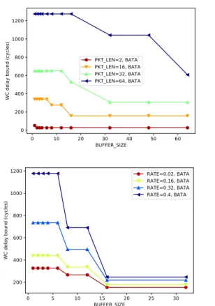
Figure 4 illustrates the end-to-end delay bounds of the foi when varying buffer size. For the top graph, we keep each flow rate constant at 4% of the total bandwidth; whereas for the bottom graph, we keep each flow payload at 16 flits.
We notice on both graphs that end-to-end delay bounds decrease with buffer size, with occasional stalling from one value to another. This is something we could expect because at a given packet length, the greater the buffer, the less a packet can spread in the network. Consequently, the IB set tends to be smaller, or to contain smaller subpaths. We notice that past a certain buffer size, the end-to-end delay bounds stay constant with larger buffers. This results from the fact that the IB set remains the same once buffers are big enough to hold an entire packet. Therefore, adding buffer space after a certain point does not improve end-to-end delay bounds. Hence, over-dimensioning the buffers within routers is not efficient to enhance NoC performance.
Next, we focus on the packet length impact on the end-to-end delay bound, as illustrated in Figure 5. The top graph presents results when the buffer size is constant (4 flits) and
0 10 20 30 40 50 60 BUFFER_SIZE 0 200 400 600 800 1000 1200
WC delay bound (cycles)
PKT_LEN=2, BATA PKT_LEN=16, BATA PKT_LEN=32, BATA PKT_LEN=64, BATA 0 5 10 15 20 25 30 BUFFER_SIZE 200 400 600 800 1000 1200
WC delay bound (cycles)
RATE=0.02, BATA RATE=0.16, BATA RATE=0.32, BATA RATE=0.4, BATA
Figure 4: Buffer size impact on end-to-end delay bounds
the bottom one when the rate of each flow is constant (4% of the link capacity).
The first observation we can make from both graphs is that the delay bounds evolve in an almost linear manner with the packet length. For instance, on the top graph, with 8 flits of buffer size and payload equal to 16, 64, 96 and 128 flits, the ratio of payload and end-to-end delay bound is 17.2, 19.9, 19.8, 19.7.
On the top graph, we observe further interesting aspects: ∙ At a given payload, the buffer size has a limited im-pact on the end-to-end delay bounds. For instance, for payload 64 flits, the delay bounds increase with less than 25% when the buffer size increases with 480%; ∙ For payloads that are significantly larger than buffer
size, the delay bound remains constant regardless of the buffer size, e.g., it is the case for payload 128 flits. Finally, we study the impact of the flow rate on the end-to-end delay bounds, as illustrated on Figure 6. The buffer size is fixed to 4 flits on the top graph and the payload to 16 flits on the bottom one. We can see on both graphs that the delay bounds increase with the rate. From the top graph, one can notice that at a constant rate, increasing the payload usually causes the end-to-end delay bound increase. On the other hand, from bottom graph, we confirm the conclusion drawn from Figure 4: increasing buffer size does not improve delay bounds after a certain value. Moreover, delay bounds seem
Flow 1 2 3 4 5 6 7 8 9 10 11 12 SRC (0, 5) (1, 5) (2, 5) (3, 5) (5, 5) (2, 4) (2, 2) (3, 4) (3, 3) (4, 4) (4, 2) (5, 2) DST (5, 4) (2, 3) (3, 2) (4, 3) (5, 1) (2, 1) (2, 0) (3, 1) (3, 0) (4, 1) (4, 0) (5, 0)
Table 1: Flow characteristics
0 20 40 60 80 100 120 PAYLOAD 0 500 1000 1500 2000 2500
WC delay bound (cycles)
BUFFER_SIZE=1, BATA BUFFER_SIZE=8, BATA BUFFER_SIZE=16, BATA BUFFER_SIZE=32, BATA BUFFER_SIZE=48, BATA
Figure 5: Payload impact on end-to-end delay bounds
more sensitive to the rate variation for small buffer sizes. For instance, for buffer size equal to 1 flit, delay bounds are 321 cycles and 1178 cycles (×3.7) for rates equal to 1% and 40% (×40), respectively. Whereas, for buffer size equal to 32 flits, the delay bounds are multiplied by only 1.6 when considering the same rate values.
The conducted sensitivity analysis reveals two main inter-esting conclusions:
∙ The configuration parameters having the highest im-pact on the derived delay bounds are the buffer size and the flow rate; Thus, both parameters will be considered for the tightness analysis;
∙ Increasing the buffer size within routers after a certain point does not improve the NoC performance; Thus, over-dimensioning the buffers is not considered as an efficient solution to decrease the delay bounds. To assess the tightness of the delay bounds yielded by BATA, we consider herein a simulation using Noxim simulator
0.00 0.05 0.10 0.15 0.20 0.25 0.30 0.35 0.40 RATE 0 1000 2000 3000 4000
WC delay bound (cycles)
PKT_LEN=2, BATA PKT_LEN=16, BATA PKT_LEN=32, BATA PKT_LEN=64, BATA 0.00 0.05 0.10 0.15 0.20 0.25 0.30 0.35 0.40 RATE 200 400 600 800 1000 1200
WC delay bound (cycles)
BUFFER_SIZE=1, BATA BUFFER_SIZE=8, BATA BUFFER_SIZE=16, BATA BUFFER_SIZE=32, BATA
Figure 6: Rate impact on end-to-end delay bounds engine [3]. Knowing no method to compute the exact worst-case for wormhole NoCs, we derive an achievable worst-worst-case delay through simulation, that we compare to the analytical end-to-end delay bounds.
In order to approach the worst-case scenario, we run each flow configuration many times while varying the flows offsets and we consider the maximum worst-case delay over all the simulated configurations. Afterwards, we compute the ”tight-ness ratio” for each flow, that is the ratio of the achievable worst-case delay and the worst-case delay bound. A tight-ness ratio of 100% means the worst-case delay bound is the exact worst-case delay. However, it is worth noticing that a tightness ratio below 100% does not necessarily mean that the worst-case delay bound is inaccurate, but it can simply reveals that the worst-case scenario has not been reached by the simulation. Therefore, the determined tightness ratio is a lower bound on the exact tightness ratio.
To perform simulations, we have configured Noxim simula-tor engine [3] to control the traffic pattern using the provided traffic pattern file option. For each flow, we have specified:
∙ the source and destination cores;
∙ 𝑝𝑖𝑟, packet injection rate, i.e. the rate at which packets are sent when the flow is active;
∙ 𝑝𝑜𝑟, probability of retransmission, i.e. the probability one packet will be retransmitted (in our context, this parameter is always 0);
∙ 𝑡on, the time the flow wakes up, i.e. starts transmitting
packets with the packet injection rate;
∙ 𝑡off, the time the flow goes to sleep, i.e. stops
transmit-ting;
∙ 𝑃 , the period of the flow.
Moreover, since we want to simulate a deterministic flow behavior to approach the worst-case scenario, we use the following parameters for each flow:
∙ Maximal packet injection rate : 1.0; ∙ Minimal probability of retransmission : 0.0;
To create different contention scenarios and try approach-ing the worst-case of end-to-end delays, we chose randomly the offset of each flow and perform simulations with uniformly distributed values of offsets for each flow. We generate 40000 different traffic configurations with random offsets for each set of parameters and simulate each of them for an amount of time allowing at least 5 packets to be transmitted.
We simulate the configuration of Figure 3, when varying buffer sizes in 4, 8 and 16 flits, and flow rates in 8% and 32% of the total available bandwidth. We extract the worst-case end-to-end delay found by the simulator and compute the tightness ratio for each flow. The obtained results are gathered in Table 2. As we can see, tightness ratio is always above 20%, while average tightness ratio is above roughly 50%. We also notice the average tightness ratio improves when the buffer size increases. For 8% rate, the average tightness ratio varies between 70.1% and 80.8%. For 32% rate, the average tightness ratio varies between 49.7% and 79.8%.
According to our sensitivity analysis, the indirect block-ing patterns covered by our model tend to become simpler when the buffer size increases, making the IB latency smaller. Moreover, we can expect a correlation between the tightness ratio and the IB set size:
∙ first, for each {flow index, subpath} pair in the IB set, the analysis may introduce a slight pessimism in the IB latency computation;
∙ second, the more complex the potential blocking sce-narios are, the harder it is to reach or approach the worst-case delay by simulations: it requires a precise synchronization between flows to achieve those sce-narios, and the greater the IB set, the less such a synchronization statistically happens over random off-sets.
Therefore, we can infer that the greater the buffer size, the easier it is to approach the worst-case delay by simulating the configuration. This is confirmed by the general trend of the average tightness ratio. It is also backed up by the following fact: in our analysis, flows 1 and 2 have the largest IB sets and are the most likely to undergo indirect blocking. We notice that at 8% rate (resp. 32% rate), their delay bounds
tightness rises from 44% to 79% (resp. 44% to 87%) and 41% to 79% (resp. 24% to 97%) when the buffer size increases from 4 flits to 16 flits.
5
COMPUTATION ANALYSIS
We now assess how well BATA scales on larger configurations through evaluating the computation time. To achieve this aim, we consider a larger NoC than the one considered for tightness analysis, while varying the number of flows. We particularly consider a 8× 8 NoC with 4, 8, 16, 32, 48, 64, 80, 96 and 128 flows and generate 20 configurations for each fixed number of flows 𝑁 . To do so, we randomly pick 2𝑁 (𝑥-coordinate, 𝑦-coordinate)-couples, where each coordinate is uniformly chosen in the specified range (here, from 0 to 7). We use 𝑁 of these couples for source cores and the other 𝑁 for destination cores. All other parameters (flow rate, packet length, buffer size, router latencies) are kept constant.
For each considered configuration, we focus on the following metrics:
∙ ∆𝑡, the total analysis runtime (computation time); ∙ ∆𝑡𝐼𝐵, the duration of the IB set analysis;
∙ ∆𝑡𝑒2𝑒, the duration of all end-to-end service curves
computations.
The derived results are illustrated in Figure 7: the top graph for ∆𝑡, the middle one for ∆𝑡𝐼𝐵 and the bottom one
for ∆𝑡𝑒2𝑒. For each flow number, we have plotted the average
runtime for all the configurations with this number of flows, as well as the computed metric for each configuration (one dot per configuration). Only configurations with runtime up to 104 s have been considered, but the IB analysis, much
faster, was performed for all configurations.
The top graph shows that the runtime grows rapidly with the number of flows (we are using a logarithmic scale on the Y-axis). Moreover, we notice that the runtimes may vary a lot for the same number of flows. For instance, for 32 flows, they range between 67ms and 110s. For 48 flows, they go from 1.5s to more than 1h10min.
To further assess what impacts the scalability of BATA, we plot the contributions to the total runtime of the IB set analysis and the end-to-end service curve computation. We notice that the IB set analysis alone (middle graph) runs in less than 8 seconds for all tested configurations. This shows that BATA approach complexity is mostly due to the end-to-end service curve computation as shown in the bottom graph. This fact is mainly due to the recursive call to end-to-end service curve function in Algorithm 1.
Computing the end-to-end service curve actually needs the computation of other service curves in two cases:
(1) when computing 𝑇𝐷𝐵, we need to know the burst of the
contending flow at the convergence point with the foi. Thus, we compute the service curve for the contending flow from its source to the convergence point with the foi (Algorithm 1, line 6);
(2) when computing 𝑇𝐼𝐵, we need to know the arrival
curve of each flow in the IB set at the beginning of its subpath. Thus, we compute the service curve of this
Rate Buffer Tightness statistics Per-flow tightness ratio
Average Max Min 1 2 3 4 5 6 7 8 9 10 11 12
8% 4 70.1% 91.7% 40.6% 44% 41% 64% 68% 77% 75% 89% 68% 47% 88% 92% 89% 8 72.1% 92.0% 38.1% 46% 38% 69% 71% 80% 79% 90% 70% 49% 90% 92% 90% 16 80.8% 88.3% 48.9% 79% 79% 85% 86% 85% 86% 87% 70% 49% 88% 88% 87% 32% 4 49.7% 95.6% 20.8% 44% 24% 51% 64% 46% 21% 44% 46% 24% 70% 96% 66% 8 64.2% 88.9% 33.3% 66% 47% 59% 81% 53% 46% 69% 65% 33% 88% 79% 85% 16 79.8% 97.3% 43.8% 87% 97% 54% 87% 64% 86% 97% 71% 44% 88% 96% 88%
Table 2: Tightness ratio results for the tested configuration
10 20 30 40 50 60 FLOW_NB values 103 102 101 100 101 102 103
104 Runtime of complete analysis (s)
RUN_TIME_TOTAL BATA Average RUN_TIME_TOTAL BATA
0 20 40 60 80 100 120 FLOW_NB values 0 1 2 3 4 5 6 7 Runtime of IB analysis (s) RUN_TIME_IB BATA Average RUN_TIME_IB BATA
10 20 30 40 50 60 FLOW_NB values 103 102 101 100 101 102 103
104 Runtime of service curve computation (s)
RUN_TIME_TIMING BATA Average RUN_TIME_TIMING BATA
Figure 7: Results of the scalability analysis
flow from its source to the beginning of the appropriate subpath (Algorithm 1, line 15).
To highlight this aspect, we measured the number of calls to the function computing a service curve during the analy-sis. The results displayed on Figure 8 and clearly show the expected trend. 10 20 30 40 50 60 FLOW_NB values 101 102 103 104 105 106 Calls to endToEndServiceCurve() CALL_NB BATA Average CALL_NB BATA
Figure 8: Number of calls to the function endToEnd-ServiceCurve()
We can also notice that when all flows are mapped on different VCs (no VC-sharing), no indirect blocking is possible, i.e. IB𝑓 = ∅ for any flow 𝑓 . Hence, there is no computation
to be done for 𝑇𝐼𝐵, which drastically reduces the complexity
of the approach in this case. In Algorithm 1, this means that lines 12 to 18 are not executed.
The derived results show that BATA gives good delay bounds for medium-scale configurations in less than one hour. However, the complexity of BATA increases with the number of flows due to the recursive calls to end-to-end service curve function. This fact is inherent to the large panel of NoCs, i.e., priority-sharing, VC-sharing and buffer backpressure, covered by BATA
6
AUTOMOTIVE CASE STUDY
In this section, we confront our model to a realistic automotive case study. This case study was used in several previous works to test NoC real-time analysis models, and recently in [13]. It consists of 38 flows on a 4 × 4 manycore platform with a 2D-mesh NoC. The parameters of the flows can be found in [2]. For convenience reasons, we reordered the flows as in [13]. We also conducted a comparative analysis with the state-of-the-art method detailed in [13] in terms of derived delay bounds tightness.
The NoC parameters used in [13] are the following: ∙ The duration of a cycle is 0.5 ns;
∙ All routers have a technological latency of 3 cycles; ∙ The link capacity is one flit per cycle;
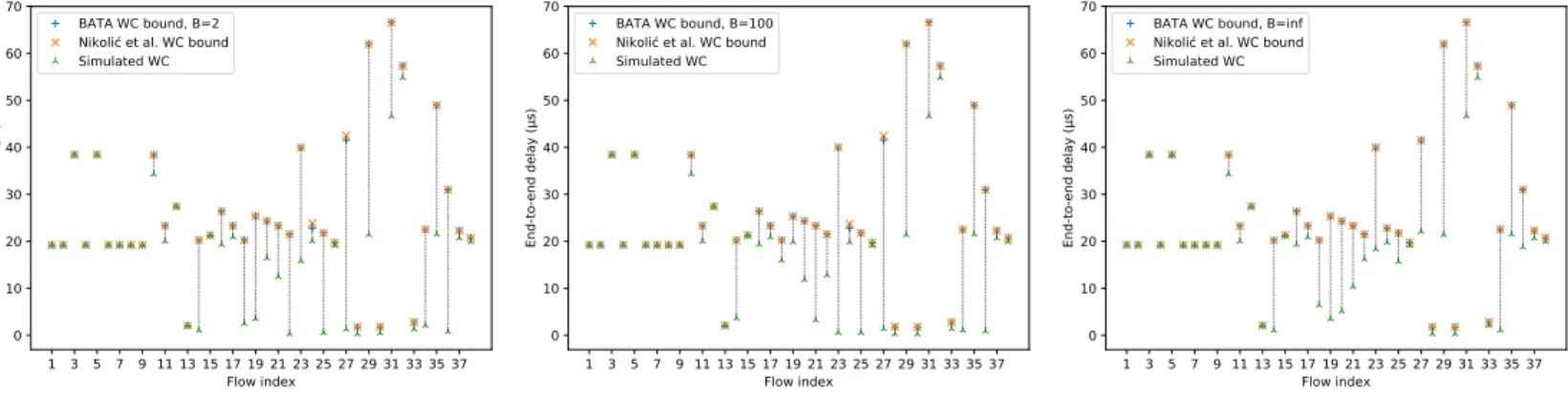
1 3 5 7 9 11 13 15 17 19 21 23 25 27 29 31 33 35 37 Flow index 0 10 20 30 40 50 60 70 End-to-end delay (µs) BATA WC bound, B=2 Nikoli et al. WC bound Simulated WC 1 3 5 7 9 11 13 15 17 19 21 23 25 27 29 31 33 35 37 Flow index 0 10 20 30 40 50 60 70 End-to-end delay (µs) BATA WC bound, B=100 Nikoli et al. WC bound Simulated WC 1 3 5 7 9 11 13 15 17 19 21 23 25 27 29 31 33 35 37 Flow index 0 10 20 30 40 50 60 70 End-to-end delay (µs)
BATA WC bound, B=inf Nikoli et al. WC bound Simulated WC
Figure 9: Worst-case end-to-end delay bounds comparison for different buffer sizes (2, 100 and ∞)
𝐵 = 2 𝐵 = 100 𝐵 = ∞ Average tightness 64% 67% 71% Average tightness difference +0.07% +0.08% -0.03% Maximum tightness difference +3.70% +3.49% +0.01% Minimum tightness difference -0.10% -0.10% -0.10% Table 3: Tightness differences for various buffer sizes between BATA and state-of-the-art approach
∙ Flows’ priority assignment follows a rate monotonic policy;
∙ Each router supports 4 Virtual Channels with no priority-sharing and no VC-sharing, i.e., one flow per VC;
∙ To compare our results to the ones in [13], we per-formed the analysis for different buffer sizes (2, 100 and 1000000 flits, the latest being large enough to assume buffer size is infinite).
We then plotted comparative graphs on Figure 9 and we notice that our approach gives similar results to [13]. To further quantify the similarity of the results, we introduce the “tightness difference” for a given flow:
∆𝜏 = 𝜏BATA− 𝜏ST ,
where 𝜏𝐵𝐴𝑇 𝐴is the tightness ratio of the bound yielded by
BATA, and 𝜏𝑆𝑇 is the tightness ratio of the bound yielded
by the method of [13]. ∆𝜏 is positive when BATA gives the tighter bound and negative otherwise. We synthesized the differences in Table 3. We computed the minimum, maximum and average tightness difference.
As we can notice, both approaches give very close results, giving credit to both models.
Authors in [13] have shown that only 4 VCs are sufficient to find a mapping of flows to VCs that ensures each flow has exclusive use of the VC within each router, which greatly simplifies the computation. However, having only one flow per VC at each node can raise scalability problems: with larger and/or less favorable configurations, ensuring each
flow has the exclusive use of a VC within each router would require a number of different VCs that is not reasonable any more.
In that respect, we want to stress out that our model allows priority sharing and VC sharing (several flows sharing prior-ity levels and VCs). Therefore, we have performed another analysis on the same configuration using only 2 VCs, with the following priority mapping:
∙ Flows 1 to 19 have the higher priority and are mapped to VC0;
∙ Flows 20 to 38 have the lower priority and are mapped to VC1.
We also analyze a configuration with only 1 shared VC. We have plotted the results with the different VC config-urations on Figure 10. We only displayed the results for a buffer size of 2 flits, but the trend is similar with other sizes. To get an insight into the impact of reducing the number of VCs on delay bounds computed with BATA, we also com-puted, for each flow and for each 𝑛 VC configuration, the relative increase of the worst-case delay bounds compared to the delay bound with 4 VCs, as follows:
𝑖𝑛𝑐𝑛 =
delay with 𝑛 VCs − delay with 4 VCs delay with 4VCs
The results are on Table 4.
First, as we can notice from Fig. 10, all flows have delay bounds less than their periods (the shortest period is 40 ms); thus remain schedulable. More particularly, when we reduce the number of VCs, the computed delay bound for each flow increases (respectively 34 and 32 times out of 38) or remains the same (respectively 4 and 1 time out of 38). However, for 5 flows cases with one VC, the computed bound decreases compared to the original configuration with no shared VC (4 VCs). The concerned flows are among the flows that have the lowest priorities in the original configuration. Mapping all flows to the same priority allows more fairness. Consequently, it tends to increase the delay bounds of the flows that had the highest priorities in the original mapping, and conversely to decrease the waiting time of lower priority flows.
1 3 5 7 9 11 13 15 17 19 21 23 25 27 29 31 33 35 37 Flow index 0 20 40 60 80 100 120 140 End-to-end delay (µs)
BATA, original 4 VCs configuration, B=2 BATA, 2 shared VCs
BATA, single shared VC
Figure 10: Delay bounds with 4, 2 and 1 VC with buffer size = 2 flits for BATA
2 VCs 1 VC Average bound increase 101.11% 145.13% Minimal bound increase 0.00% -95.05% Maximal bound increase 464.16% 2293.01% Table 4: Relative increase of the worst-case end-to-end delay bounds for 𝐵 = 2 with BATA
Moreover, in Table 4, we compute the average increase of the worst-case delay bounds computed with BATA when we reduce the number of VCs, compared to the bound with 4 VCs. The average bound increase stays reasonable (up to 150 %) when the number of available VCs is divided by 2 or 4. In comparison to the state-of the-art method in [13], BATA does not need the non-shared VCs assumption; thus, BATA enables the delay bounds computation with shared VCs. In this particular case study, we are able to show that decreasing the number of Virtual Channels (and consequently the platform complexity) can be done while maintaining the schedulability of all flows and complying with the timing constraints.
Finally, we provide some insights into the runtime of our method. For each buffer size and number of VCs, we measured the runtime of our analysis and summarized our results in Table 5. We notice that runtimes with non-shared VCs are in the order of 10 times lower than runtimes with 1 and 2 VCs. This confirms our conclusions in Section 5 concerning the inherent complexity of BATA to handle the priority-sharing and VC-sharing assumptions.
Actually, when no VC is shared between several flows, the IB latency is zero. However, when VCs are shared, there are additional recursive calls to end-to-end service curve function needed to compute the IB latency; thus we can expect an increase in the analysis duration.
7
CONCLUSION
In this paper, we proposed an extensive evaluation of the tightness and computation time of our previously published
4 VCs 2 VCs 1 VC Runtime (ms) 𝐵 = 2 6.36 55.4 84.6 𝐵 = 100 6.30 125.0 144.4 𝐵 = ∞ 6.20 62.4 84.4 Table 5: Runtimes of BATA for different NoC con-figurations when sharing VCs
buffer-aware worst-case timing analysis (BATA) for wormhole NoCs [5]. To evaluate the tightness, we first studied how the various system parameters impact the computed end-to-end delay bounds. We found our model to be most sensitive to rate and buffer size. Consequently, we proceeded the tightness analysis with a set of different buffer sizes and flow rates. We were able to achieve a tightness ratio up to 80% on average, with reference to simulation.
We then estimated the scalability of our approach in terms of computation time when increasing the number of flows. We found that the main complexity of the analysis lies in the indirect blocking latency computation, as it leads to additional recursive calls to the function computing the end-to-end service curve. However, this complexity comes from the fact that the model is able to cover configurations with shared priority and shared VCs. If no VCs are shared, the analysis is much less complex.
Finally, we compared our results to those of [13] on an au-tomotive case study. We have shown that the results are very similar, with tightness ratios differing by less than 0.1% on average. Moreover, since our model is not limited by the as-sumptions of no priority-sharing and no VC-sharing, we have analyzed other configurations with reduced number of VCs (thus lower complexity) while maintaining the schedulability
of all flows.
Our next focus will be to rethink the indirect blocking analysis in order to decrease the computational cost of BATA while covering a large panel of NoC configurations.
REFERENCES
[1] Abdallah, L., Jan, M., Ermont, J., and Fraboul, C. Wormhole networks properties and their use for optimizing worst case delay analysis of many-cores. In 10th IEEE International Symposium on Industrial Embedded Systems (SIES) (June 2015), pp. 1–10. [2] Burns, A., Indrusiak, L. S., and Shi, Z. Schedulability analysis for real time on-chip communication with wormhole switching. Int. J. Embed. Real-Time Commun. Syst. 1, 2 (Apr. 2010), 1–22. [3] Catania, V., Mineo, A., Monteleone, S., Palesi, M., and Patti,
D. Cycle-accurate network on chip simulation with noxim. ACM Trans. Model. Comput. Simul. 27, 1 (Aug. 2016), 4:1–4:25. [4] Ferrandiz, T., Frances, F., and Fraboul, C. A method of
com-putation for worst-case delay analysis on spacewire networks. [5] Giroudot, F., and Mifdaoui, A. Buffer-aware worst-case
tim-ing analysis of wormhole nocs ustim-ing network calculus. In 2018 IEEE Real-Time and Embedded Technology and Applications Symposium (RTAS) (Porto, PT, 2018), pp. 1–12.
[6] Jafari, F., Lu, Z., and Jantsch, A. Least upper delay bound for vbr flows in networks-on-chip with virtual channels. ACM Trans. Des. Autom. Electron. Syst. 20, 3 (June 2015), 35:1–35:33. [7] Le Boudec, J.-Y., and Thiran, P. Network Calculus: A Theory of
Deterministic Queuing Systems for the Internet. Springer-Verlag, Berlin, Heidelberg, 2001.
[8] Liu, M., Becker, M., Behnam, M., and Nolte, T. Tighter time analysis for real-time traffic in on-chip networks with shared priorities. In 10th IEEE/ACM International Symposium on
Networks-on-Chip (2016).
[9] Mifdaoui, A., and Ayed, H. Buffer-aware worst case timing analy-sis of wormhole network on chip. arXiv abs/1602.01732 (2016). [10] Mohapatra, P. Wormhole routing techniques for directly con-nected multicomputer systems. ACM Comput. Surv. 30, 3 (Sept. 1998), 374–410.
[11] Ni, L. M., and McKinley, P. K. A survey of wormhole routing techniques in direct networks. Computer 26, 2 (Feb 1993), 62–76. [12] Nikoli´c, B., Ali, H. I., Petters, S. M., and Pinho, L. M. Are virtual channels the bottleneck of priority-aware wormhole-switched noc-based many-cores? In RTNS (2013).
[13] Nikolic, B., Tobuschat, S., Soares Indrusiak, L., Ernst, R., and Burns, A. Real-time analysis of priority-preemptive nocs with arbitrary buffer sizes and router delays. Real-Time Systems (06 2018).
[14] Qian, Y., Lu, Z., and Dou, W. Analysis of worst-case delay bounds for best-effort communication in wormhole networks on chip. In Networks-on-Chip, 3rd ACM/IEEE International Symposium on (May 2009).
[15] Rambo, E. A., and Ernst, R. Worst-case communication time analysis of networks-on-chip with shared virtual channels. In Proceedings of Design, Automation Test in Europe Conference
Exhibition (2015).
[16] Schmitt, J. B., Zdarsky, F. A., and Martinovic, I. Improving performance bounds in feed-forward networks by paying multi-plexing only once. In 14th GI/ITG Conference - Measurement, Modelling and Evalutation of Computer and Communication Systems (March 2008), pp. 1–15.
[17] Shi, Z., and Burns, A. Real-time communication analysis for on-chip networks with wormhole switching. In Networks-on-Chip, Second ACM/IEEE International Symposium on (April 2008). [18] Shi, Z., and Burns, A. Real-time communication analysis with a priority share policy in on-chip networks. In 21st Euromicro Conference on Real-Time Systems (July 2009), pp. 3–12. [19] Tobuschat, S., and Ernst, R. Real-time communication analysis
for networks-on-chip with backpressure. In Design, Automation Test in Europe Conference Exhibition (2017).
[20] Wentzlaff, D., Griffin, P., Hoffmann, H., Bao, L., Edwards, B., Ramey, C., Mattina, M., Miao, C. C., III, J. F. B., and Agarwal, A. On-chip interconnection architecture of the tile processor. IEEE Micro 27, 5 (Sept 2007), 15–31.
[21] Xiong, Q., Wu, F., Lu, Z., and Xie, C. Extending real-time analysis for wormhole nocs. IEEE Transactions on Computers PP, 99 (2017), 1–1.