Learning-by-Doing in an Ambiguous Environment

Texte intégral

(1)2006s-29. Learning-by-Doing in an Ambiguous Environment Jim Engle-Warnick, Sonia Laszlo. Série Scientifique Scientific Series. Montréal December 2006. © 2006 Jim Engle-Warnick, Sonia Laszlo. Tous droits réservés. All rights reserved. Reproduction partielle permise avec citation du document source, incluant la notice ©. Short sections may be quoted without explicit permission, if full credit, including © notice, is given to the source..

(2) CIRANO Le CIRANO est un organisme sans but lucratif constitué en vertu de la Loi des compagnies du Québec. Le financement de son infrastructure et de ses activités de recherche provient des cotisations de ses organisations-membres, d’une subvention d’infrastructure du Ministère du Développement économique et régional et de la Recherche, de même que des subventions et mandats obtenus par ses équipes de recherche. CIRANO is a private non-profit organization incorporated under the Québec Companies Act. Its infrastructure and research activities are funded through fees paid by member organizations, an infrastructure grant from the Ministère du Développement économique et régional et de la Recherche, and grants and research mandates obtained by its research teams. Les partenaires du CIRANO Partenaire majeur Ministère du Développement économique, de l’Innovation et de l’Exportation Partenaires corporatifs Alcan inc. Banque de développement du Canada Banque du Canada Banque Laurentienne du Canada Banque Nationale du Canada Banque Royale du Canada Banque Scotia Bell Canada BMO Groupe financier Bourse de Montréal Caisse de dépôt et placement du Québec DMR Conseil Fédération des caisses Desjardins du Québec Gaz de France Gaz Métro Hydro-Québec Industrie Canada Investissements PSP Ministère des Finances du Québec Raymond Chabot Grant Thornton State Street Global Advisors Transat A.T. Ville de Montréal Partenaires universitaires École Polytechnique de Montréal HEC Montréal McGill University Université Concordia Université de Montréal Université de Sherbrooke Université du Québec Université du Québec à Montréal Université Laval Le CIRANO collabore avec de nombreux centres et chaires de recherche universitaires dont on peut consulter la liste sur son site web. Les cahiers de la série scientifique (CS) visent à rendre accessibles des résultats de recherche effectuée au CIRANO afin de susciter échanges et commentaires. Ces cahiers sont écrits dans le style des publications scientifiques. Les idées et les opinions émises sont sous l’unique responsabilité des auteurs et ne représentent pas nécessairement les positions du CIRANO ou de ses partenaires. This paper presents research carried out at CIRANO and aims at encouraging discussion and comment. The observations and viewpoints expressed are the sole responsibility of the authors. They do not necessarily represent positions of CIRANO or its partners.. ISSN 1198-8177. Partenaire financier.

(3) Learning-by-Doing in an Ambiguous Environment * Jim Engle-Warnick †, Sonia Laszlo‡ Résumé / Abstract Une étude expérimentale a été menée afin de tester si l’aversion au risque ou l’aversion à l’ambiguïté peuvent expliquer les décisions prises par les sujets lors d’un jeu d’apprentissage par essais. Nous avons d’abord mesuré la préférence des sujets face au risque et à l’ambiguïté, et avons ensuite utilisé ces mesures pour prédire le comportement des sujets au cours du jeu. Nous avons pu constater que les sujets qui éprouvent de l’aversion à l’ambiguïté décident de payer plus souvent afin de clarifier cette ambiguïté. D’autre part, nous avons constaté que moins les sujets éprouvent de l’aversion au risque, plus leurs gains lors du jeu sont élevés. À la lumière d’une étude sur le terrain ayant eu lieu avec des fermiers travaillant dans une économie en développement, nos résultats confirment l'évidence d'un lien entre l'aversion à l'ambiguïté et les choix technologiques, ainsi que d'un lien entre l'aversion au risque et la rentabilité d'une ferme. Mots clés : apprentissage par essais, choix technologiques, préférences vis-àvis du risque, instruments de mesure du risque, aversion à l’ambiguïté, économie expérimentale. We experimentally test whether risk aversion or ambiguity aversion can explain decisions in a learning-by-doing game. We first measure subjects' preferences toward risk and ambiguity, and then use these measures to predict behavior in the game. We find that ambiguity averse subjects pay more often to resolve ambiguity, and we find that less risk averse subjects earn more in the game. Our results, in light of a previous field study of farmers in a developing economy, provide further evidence of a link between ambiguity aversion and technology choice, as well as a link between risk aversion and farm profitability. Keywords: learning-by-doing, technology choice, risk preferences, risk measurement instruments, ambiguity aversion, experimental economics Codes JEL : C91, D80. *. We thank Claude Montmarquette, Peter Moffatt, and participants at the 2006 Economics Science Association European Meetings in Nottingham. We thank Duncan White-head for research assistance. We gratefully acknowledge the Social Science and Humanities Research Council of Canada for funding, and the Centre for Interuniversity Research and Analysis on Organizations (CIRANO) and the Bell University Laboratory in Electronic Commerce and Experimental Economy. † Department of Economics, 855 Sherbrooke St. West, McGill University, Montreal, Quebec, H3A 2T7, Canada, e-mail: jim.engle-warnick@mcgill.ca; tel.: (514) 398-1559; fax: (514) 398-4938. ‡ Department of Economics, 855 Sherbrooke St. West, McGill University, Montreal, Quebec, H3A 2T7, Canada, e-mail: sonia.laszlo@mcgill.ca; tel.: (514) 398-1924; fax: (514) 398-4938..

(4) 1. Introduction. The adoption of new technologies is a fundamentally important issue for economies. From farmers’ decisions to switch to new seeds, to the choice of computer technology, to contraceptive choice, to the diffusion of technology throughout an economic sector, new technology adoption is a widely studied and important phenomenon. For example, it has long been accepted that farmers in developing countries are slow to adopt new technologies. Among many competing hypotheses, risk aversion is viewed as an important determinant of technology adoption (Feder et al. (1985) and subsequent literature). Because they are poor and thus have little recourse to credit or insurance markets, subsistence farmers tend to be relatively risk averse. Important evidence for this idea came from Binswanger (1980) who, in his well-known experiment with choices between lotteries, established the existence of a group of farmers in India whose measured preferences were indeed risk averse. While risk aversion can explain a preference to not choose new ways of doing things, it is difficult to make the connection between risk preference and technology choice. This is because risk preferences are neither observable nor typically formally revealed in survey data. Many field studies have compensated by using a combination of survey questions on risk attitudes and modeling assumptions to correlate measures of risk with technology choice (e.g., Knight, Weir, and Woldehanna (2003), Antle and Crissman (1990), and Feder, Just, and Zilberman (1985) for a survey). Results from these studies normally find a negative correlation between risk aversion and new technology adoption. A recent field study took a further step by combining a Binswanger-like laboratory experiment in the field with a socioeconomic survey to correlate an incentivized behavioral measure of risk with technology decisions reported in the survey. With this methodology, Engle-Warnick, Escobal and Laszlo (2006) provided evidence that in their sample of farmers, it is not actually risk aversion but aversion toward ambiguity that predicts seed technology.

(5) decisions on the farm.1 Furthermore, among competing hypotheses typically explored in the context of farming in developing countries, learning-by-doing was found to be an important mechanism through which farmers made new technology decisions.2 The inference is that farmers learn about other technologies as they gain experience with one of them, and that they view unknown technologies as having unknown probability distributions over possible outcomes. Farmers apparently learn by doing in an ambiguous environment. This result is surprising given the reliance on the hypothesis that risk aversion drives such results. This result is new because it relies on both the field laboratory experiment and the survey results from the same subject to correlate the measure with the decision. However, evidence from this study is indirect in the sense that we do not really know that the farmers see the technology choice as ambiguous in the way that we define it as ambiguous, nor do we have direct measurable data regarding their technology choice. By contrast, in the traditional experimental laboratory we can present subjects with a truly ambiguous learning-by-doing environment, and in this paper this is precisely what we do. The idea is to explore further the connection between ambiguity preferences and new technology choice. The advantage of this study compared with others is that, while it is informed by field results, all the data are collected under the control of the experimental laboratory. In our experiments subjects first report for a session during which they respond to individual choice problems under uncertainty to measure their risk and ambiguity preferences. The instruments are standard: to measure risk preferences, subjects are asked to choose between risky and safe lotteries, and to measure ambiguity preferences, subjects are given the option to buy their way out of playing ambiguous lotteries, i.e., lotteries with unknown probability distributions over outcomes. 1. Using incentivized laboratory measures of risk and time preferences are becoming increasingly used both to predict decisions in laboratory games in the field (e.g., Barr for behavior in games (2003), and Eckel, Johnson, and Montmarquette (2004) to predict decisions in the field). 2 See Foster and Rosenzweig (1995) for other examples of such a finding.. 2.

(6) The subjects are then recalled a month later to play a technology choice game. In the game, as the subjects use a technology, they learn in a noisy way about a more efficient technology. The sole decision is when to switch from the first technology into the more efficient one.3 When to switch is ambiguous: the subjects do not know the probability distribution of earnings for the possible switch times, thus they must gain experience with the game to resolve the ambiguity. Resolving ambiguity comes at a nominal cost. We report two main findings. First, our measure of ambiguity aversion is correlated to the degree to which subjects are willing to incur a cost to reduce ambiguity in the learningby-doing game. This is important, because it suggests that the ambiguity aversion measure is measuring what is intended. Second, risk aversion is negatively correlated with performance, measured by net earnings, in the learning-by-doing game. This is surprising, and suggests both further exploration into the mechanism that causes this result, and further exploration into whether this is also true in the field. With this test of the learning-by-doing model of Jovanovic and Nyarko (1996), we provide the following contributions. First, we confirm that the ambiguity aversion measure is robust to the changes in framing between the two experiments. This gives us some confidence that it is measuring the predispositions that we wish it to measure. Second, we learn that risk preferences predict profits in a game that was motivated by a field study and designed to shed light on the field decision. This begs the question whether this result would hold up in the field. Third, our paper illustrates the possibility of continuing interaction between the traditional experimental laboratory and a laboratory in the field in a developing economy, with the traditional laboratory not only providing the possibility of sharper tests of field discoveries, but also making predictions that are testable back in the field.4 Our original 3. The learning model is due to Jovanovic and Nyarko (1996). Experimental tests of learning-by-doing have typically focused on fitting dynamic learning models to choice data: Camerer (2003) provides a survey. Merlo and Schotter (2003) provide an experimental test, using a model similar in spirit to Jovanovic and Nyarko (1996), of whether observational learning of an agent who is learning-by-doing can be an efficient form of learning. 4 Other studies provide links between the laboratory and the field. For example, Kagel and Roth (2000). 3.

(7) field study, which made use of both a field laboratory and a survey to measure decisions on the farm, resulted in a surprising finding, i.e., that ambiguity preferences predict technology choice. Because the result was new, and because it is rarely known precisely what a behavioral measure is actually measuring, we appealed to the control of the traditional experimental laboratory to better understand our measure. Not only did we validate, in a sense, the measure, but we developed another hypothesis to take with us back to our laboratory in the field. We also provide a methodological contribution with demonstration of a method to handle inference with a highly skewed distribution of payoffs. Because subject payoffs are determined by a quadratic loss function in the learning-by-doing model, the distribution of payoffs is not normal. We illustrate a method to transform the variables to correct for this, and to estimate marginal effects with the transformation. For models with quadratic functions determining payoffs this method may be useful. The next section describes the experiment for measuring risk and ambiguity preferences. The following section describes the learning-by-doing experiment, which was conducted approximately one month later. We then present the experimental results and conclude.. 2 2.1. Preference Measurement Experimental Design Risk Preference Measure. We derive our instrument of risk preference measure from the instrument in Figure 1, which we denote ‘five options’ (FO hereafter). An instrument similar to this Binswanger-like instrument was introduced by Eckel and Grossman (2003). Five options, each represented by a circle, are presented to the subject, who is instructed to select exactly one of them. Each report a study in which a laboratory experiment is conducted to isolate the effect of an institution on decisions in a labor market. The study provided support for implementing a new institution in the field.. 4.

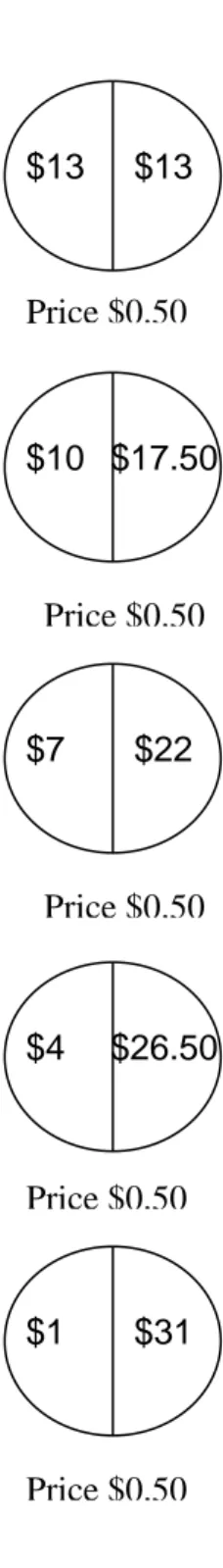
(8) option contains two payoffs, separated by a vertical line. The vertical line indicates that each payoff has a 50% probability of occurring: in the top option for instance, subjects earn $13 CAD with certainty, while the option to its left has a low payoff of $10 (with 50% probability) and a high payoff of $17.50 (with 50% probability). As one moves counter clockwise in this figure, the variance in the payoffs increases. For our measure of risk preferences, which we denote ‘risk measure’ (RM), we decomposed FO into a set of four binary choices. This decomposition resembles the instrument in Holt and Laury (2000). The measure is presented in Figure 2, where each row in the figure represents one binary choice between gambles. In fact, each choice is between two alternatives that were located next to each other in the circle of FO. Beginning with the first row of choices and moving down, an expected utility maximizer will at some point switch from the left-hand side gamble with lower variance to the right-hand side gamble with a higher variance and slightly higher expected utility. The sooner the subject switches from the left-hand side to the right-hand side, the less relatively risk averse she is.5. 2.2. Ambiguity Preference Measure. Our second instrument, which we denote Ambiguity Measure (AM) is designed to measure preferences about ambiguity. Figure 3 shows the collection of these five decisions, one in each row. In the figure, the gamble on the left displays the possible prizes, but not the probability of winning those prizes (this unknown probability distribution is communicated by eliminating the vertical line in the center of the circle). The gamble on the right contains the same prizes, but with a 50/50 chance of winning each one. However, if a subject chooses the gamble on the right, she must pay $0.50 of her final earnings back to the experimenter 5. We decomposed FO into RM to use the relatively simple 50/50 choice gambles within a framework within which we could study the effect of adding additional alternatives to the choice set. We used the simplest design we could, i.e., one with 50/50 gambles because we later replicated this experiment in rural Peru.. 5.

(9) for making this choice.6 Thus the left gamble is ambiguous because the subject does not know the probability distribution over outcomes, and the costly right gamble provides the subject with an opportunity to reveal her preference to avoid this ambiguity.7. 2.3. Explanatory variables generated by the experiment. First, to measure risk preferences, we take the four decisions depicted in Figure 2, noting that each decision is a choice between a relatively safe and a relatively risky gamble. For the risk preference measure we simply count the number of risky choices made by the subject. The fewer risky choices, which can take on integer values from zero to four, the less risk averse a subject is. This measure is equivalent to the one used by Holt and Laury (2002), and is analogous to finding the gamble the subjects would have chosen in the Five Circles instrument. Second, to measure ambiguity preferences, precisely as in our measure of risk preferences, we count the number of times subjects pay to avoid an ambiguous gamble in each of the five choice problems shown in Figure 3. This measure takes on integer values from zero to five. The more subjects are averse to ambiguity, the higher this measure. For a simple model of decision making, one can think of a subject who has a predisposition against ambiguity. The higher this predisposition, the more likely the subject is to pay to avoid it, thus the more often the subject will, on average, pay to avoid it. 6. In no case can this ever result in a negative payoff for choices in the experiment. Perhaps the most standard method for measuring preferences for ambiguity is to elicit subjects’ willingness to pay for both the ambiguous and non-ambiguous gambles, and take the measure as the difference between the two valuations. This design, which would require the use of the Becker, DeGroot, and Marschak (1964) procedure of elicitation, would be more complicated and it is unclear if it would result in less noisy responses. Another way would be to fix the ambiguous gamble and vary the cost for choosing the unambiguous gamble. These two designs have their merits, as they return a price level as the measure. We chose our simpler design with multiple gambles and a single price to avoid ambiguity because it is easy to derive a measure from, and because it enabled our ambiguity measure to most closely mirror our risk preference measure. 7. 6.

(10) 2.4. Experimental Procedures. The sessions were conducted with paper and pencil. Subjects were given a book with one decision to make on each of forty-four pages.8 The pages were randomly ordered, as was the left to right presentation of the gambles, and the instructions were given orally. Subjects indicated their decisions by placing a mark above their choice in their booklet, and an experimenter verified that there was exactly one choice made on each page when completed. To prevent influencing the results, the subjects were not informed in advance that their booklets would be verified. Subjects were privately paid for one randomly chosen decision. All payoffs were displayed in Canadian dollars. We conducted six sessions, which were run at a university experimental laboratory. The subjects were recruited by e-mail from the English-speaking subject pool (the laboratory also has a French-speaking subject pool). Subjects were paid a $10 show up fee upon arrival before making their decisions, and the same experimenter conducted the sessions and read the script to the subjects in all the sessions. One-hundred and six subjects participated in this experiment, with session sizes of approximately fifteen to twenty. Subjects earned an average of $20 in addition to the $10 show up fee. The experiments lasted approximately one hour.. 3. Learning-by-Doing Experimental Design. Approximately one month after completing the preference measure experiment, subjects were recalled to play the learning-by-doing game. The subjects were not informed that the second experiment was related to the first experiment. 8. The experimental design consists of an additional set of questions that study the effect of additional choices. In addition to the risk and ambiguity measures, there were decisions to reveal the effect of additional alternatives on choice, and to reveal preferences for payoff dominated alternatives. The effect for this experimental study was to randomly scatter the nine questions we are interested in here among thirty-five other questions. The complete choice booklet is available upon request from the authors. For a description of the additional alternative aspect of the design, see Engle-Warnick, Escobal, and Laszlo (2006).. 7.

(11) 3.1. Learning-by-Doing Model. The learning-by-doing model we use was introduced by Jovanovic and Nyarko (1996). In this model, a firm learns about a parameter of a technology by using the technology. At the same time the firm learns in a noisy way about a parameter of a more efficient technology. Think of a farmer planting seeds at the beginning of a growing season, with more modern and efficient varieties available. Learning how to plant the traditional seed assists with learning some aspects about how to plant the modern seed. But the learning is noisy, because choices such as type of irrigation and type of fertilization might be different with the modern seed. This same model has been used in the economic development literature concerned with technology adoption for situations such as these (e.g., Foster and Rosenzweig (1995) and Rosenzweig (1995)). The game is played repeatedly, where the firm chooses to continue with the least efficient technology (technology 1), or to permanently switch to the more efficient one (technology 2). Whichever technology the firm chooses, it must also choose an intensity of use. Switching from the first technology to the more efficient technology results in an immediate loss in profits, because learning about the more efficient technology is noisy, and the firm’s prior for the optimal intensity of use is thus inaccurate. However, switching also results in the opportunity to earn higher profits in the long term, because learning will be faster, and because of the efficiency gain. Formally, the payoff, q, to the firm is determined by a quadratic loss function, which measures the time t difference between the firm’s selected intensity of technology use, x, and an optimal intensity of use, yt , which is randomly determined:. q = γ n [a − (yt − x)2 ], γ > 1. (1). The parameter γ determines the increase in efficiency from a new technology, where the available technologies are indexed by the integer n. At time t, the firm selects x, then sees 8.

(12) q, at which time it can update its beliefs with Bayes’ rule about the technology parameter θn by inferring yt . The optimal choice for technology intensity is yt , and this optimal level is determined by the technology specific parameter θn and a random variable:. yt = θn + wt. (2). where wt is normally distributed i.i.d. with zero mean. The technologies are linked through θ:. θn+1 =. √. αθn + ²n+1. (3). The optimal behavior of the firm involves using Bayes’ rule to update its belief about x = E[yt ] = Et [θt ] each time it observes its payoff q. At some point, the immediate cost of switching no longer exceeds the future cumulative gains from efficiency, and the firm should switch. If the firm switches too soon, it loses profits from not having learned enough. If the firm switches too late, it loses profits from efficiency gains.. 3.2. Experimental Procedures. The experiment was programmed and conducted with the software z-Tree (Fischbacher 1999). The subjects played the learning-by-doing game for twenty-five rounds. Their sole decision was which period to switch from the less efficient technology (technology 1) to the more efficient technology (technology 2). In our implementation of this game, we gave the computer a prior over the optimal use of technology 1 (x), and allowed the computer to update its prior using Bayes’ Rule for both technologies after the realization of the optimal use (yt ) each round. The computer played its estimate of x, the period payoff was realized, then the computer updated its new estimate of x for both technologies. Our design thus limited the subjects’ strategy to finding the optimal switch-point from technology 1 to technology 2. 9.

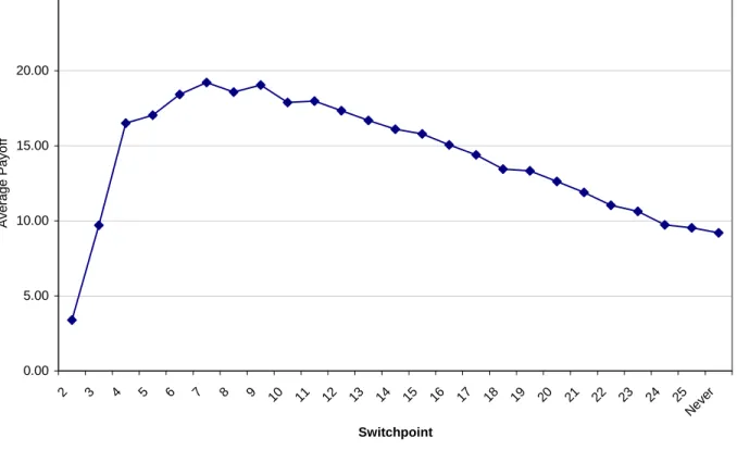
(13) The subjects’ computer display included the round number, the technology currently in use, the computer’s estimate of x for the technology currently in use, the period realization of the optimal use, the period payoff, the total payoff for all periods played, and the computer’s estimate of x for technology 2 (this last information reminded the subjects that the computer was learning about the unused technology as long as technology 1 was in use). Once the subjects switched to technology 2, they were not permitted to switch back. The challenge in implementing this model is to find parameters that result in a steep enough surface of maximization to be behaviorally meaningful. Quadratic loss functions, which are flat at the maximum, can be poor with regard to providing economic incentives for human subjects to optimize. We chose the following parameters for the model: a = 50; γ = 1.8; α = 20; ² ∝ N (0, 0.25); w ∝ N (0, 0.25) We played our game, switching thirty times after each period of the twenty-five period game, and computed an average payoff for switching in each period. This computation, which reports actual values from our computer program that implemented the experiment, is shown in Figure 4. Figure 4 confirms that our chosen model parameters result in a fairly steep surface of maximization with a switch period that should not be easily guessed by the subjects. The theoretical optimal switch-period is t = 8, and the maximum expected payoff is approximately $20. The worst thing to do is to switch right away; this is because at this point not enough has been learned about the optimal intensity of use of technology 2. In the instructions the subjects were informed that the task was to choose whether or not (and when) to switch to technology 2 in a twenty-five period game. The subjects were shown the loss function that determined their payoffs so that in theory they were aware that the payoff function was smooth and contained a unique maximum. The subjects were told that the computer updated its information and learned about both technologies. The subjects were not given equations (2) or (3), i.e., they knew neither the process generating the optimal intensity of use, nor the way the technologies were linked. 10.

(14) Notice that in this game, there is a distribution for the payoff for each possible switch point. To the subjects, this distribution is unknown because they did not have full information about the model. Thus, this information condition is the basis for making the technology choice environment ambiguous. Subjects who pay to avoid ambiguity in the preference measurement experiment should also pay to resolve this payoff ambiguity in the learning-by-doing experiment. After setting out the decision making problem, the instructions then informed the subjects that they could pay $0.50 to practice the game for no pay as many times as they wanted. This gave the subjects the opportunity to resolve the ambiguity regarding when to switch from technology 1 to technology 2, at a low cost. Our question is whether we can use our preference measures from the first experiment to predict behavior and performance in the second experiment. We conducted seven sessions, which were run at a university experimental laboratory. The subjects were recruited by e-mail from the group of subjects who previously participated in the preference elicitation experiment. Subjects were paid a $10 show up fee. Seventy-two subjects participated in the experiments. Subjects earned an average of $15.40 in addition to the $10 show up fee. The experiments lasted approximately one hour.. 4. Experimental Results. 4.1. Preference Measurement Experiment. In what follows, we restrict the sample to the 72 subjects who participated in both sets of experiments (i.e., the preference measurement and the learning-by-doing experiments).9 De9. The subjects who did not participate in the learning-by-doing experiments are no different in their observed socio-economic conditions or in their responses to the preference experiments than those that did. We confirmed this by using t-tests for all independent variables, and in no case were we able to reject that the included sample of 72 observations is any different than the excluded sample of 34 observations.. 11.

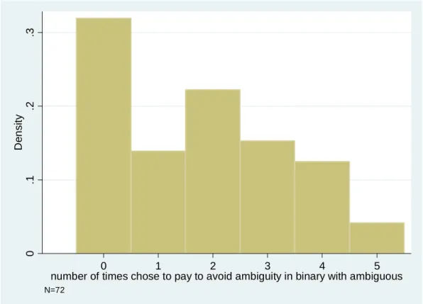
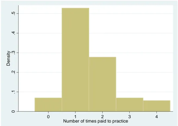
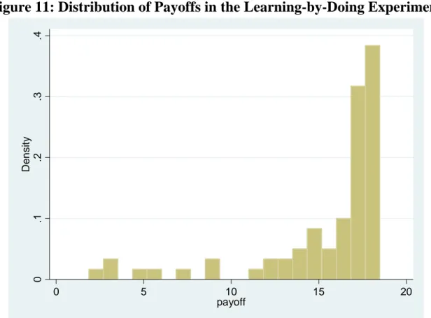
(15) scriptive statistics of the observed socio-economic characteristics of this sample are provided in the appendix. Figure 5 shows a histogram of the number of risky decisions made by the subjects in the binary gamble. The figure reveals heterogeneity in decision-making, with subjects choosing all possible numbers of risky choices from zero to four. There is a mode at one risky choice, and the second-most chosen number of safe choices is two. We also split the sample by gender as a validity check of our results. The common finding in laboratory experiments is that women measure more risk averse than men, and indeed Figure 6 confirms that this is the case in our sample. Figure 7 presents a histogram of the number of times subjects paid to avoid an ambiguous gamble. There is a mode at zero, but roughly two thirds of the subjects paid to avoid the ambiguous gamble at least once. Again, splitting the sample by gender we find in Figure 8 that women tend to be more willing to pay to avoid ambiguity than men. The average number of times women paid to avoid the ambiguous gamble was 1.89, compared with an average of 1.48 for men. Both measures imply a great deal of heterogeneity, giving the possibility of having some predictive value. We now turn to the results from the learning-by-doing experiment.. 4.2. Learning-by-Doing Experiment. Figure 9 presents a histogram of the number of times subjects paid to practice the learningby-doing game. There is a mode at one, and the second-most number of times practicing is two. Five subjects did not practice the game at all, and nine subjects practiced three or four times. Distributions are similar for men and women, shown in Figure 10. Figure 11 presents the distribution of payoffs, which is skewed to the right. This distribution is driven by the quadratic loss function (see equation (1) on page 9). To see this, recall Figure 4, which revealed a steep climb to the left of the optimal switch point of eight rounds, 12.

(16) and a relatively flat area to its right. One could choose a switch point of six through fifteen rounds and expect to earn at least $15 in the experiment. Finding the optimal point adds approximately $5 in expectation to earnings, which is not trivial. However, a subject who experiments with moving the switch point down from later rounds (say, from round fifteen to round fourteen or thirteen), will find that reinforcement from experimentation may result in small increases to earnings, thus may stop experimenting. And many subjects may find themselves closer to the maximum with very similar earnings. Thus without strong economic incentives to find the maximum, and with many switch points resulting in near-optimal earnings, we may expect to find the earnings of many subjects who play the game relatively well to be clustered in this range, and Figure 11 reveals that this is indeed the case. Furthermore, approximately two-thirds of our subjects earned payoffs in the range between $17 and $18, and these payoffs occur at the flattest part of the payoff function. Those subjects who do not do as well we find scattered to the left of this range. These relatively few subjects switch very early or very late, where the range of payoffs is larger. Our belief is that a non-normal distribution of payoffs may occur with a combination of this type of economic incentive and heterogeneous subjects. Our empirical analysis will take the non-normality of payoffs into account.10. 4.3. Ambiguity Aversion Measure. One important question is whether the subjects saw the ambiguity aversion instrument decision making problem as similar to the decision to pay to reduce ambiguity in the learningby-doing experiment. If not, then we would be concerned that decision making is too noisy to help with predictions, or that the measure was not robust to a change in the framing of the problem. It turns out that the decisions are positively and significantly correlated. We 10. For another example of this type of result, Engle-Warnick and Turdaliev (2006) find a similar payoff distribution in a central banking game, which uses a quadratic loss function. They accounted for this by performing a regression analysis for each individual subject.. 13.

(17) show this in two ways. First, the correlation between the ambiguity measure taken from the preference experiment and the number of times subjects paid to practice in the learning-by-doing is 0.2061 (with a significance level of 0.0824). This provides some evidence that paying to avoid ambiguity is positively correlated with paying to practice the learning-by-doing game. Table 1 reveals additional evidence of the positive association between the ambiguity aversion measured in the preference measurement experiment and the number of times practiced in the learning-by-doing experiment. The table reports results from an ordered probit of the latter on the former, including session controls. Our results indicate that the number of times subjects paid to avoid the ambiguity positively predicts the number of times they practiced. Table 1 also reports the marginal effects from this exercise. We find that subjects who are ambiguity averse are less likely to never practice or practice only once, but more likely to practice two or four times. While we cannot say what the correlation between these two measures should be, we can say they move together in the same direction. This is what we should expect if the two decisions are both seen as similar with regard to ambiguity. We next use the preference measures to predict performance in the game.. 4.4. Predictive Results. We wish to investigate the effects of risk preference (RM ), ambiguity aversion (AM ) and the number of times the subjects practiced (N P ), on the payoffs (y) earned by each subject. To do so, we are interested in estimating the following regression:. y = X0 β + ². (4). where X = [RM, AM, N P, Z], Z a vector of control variables and ² a random disturbance term. In columns (1) and (2) of Table 2 we present the results from estimating (4) by 14.

(18) ordinary least squares. The model estimated in column (1) does not contain socio-economic controls, while the model estimated in column (2) does. We find that more risk loving individuals have higher payoffs, while subjects that practice more have lower payoffs. Specifically, subjects who practiced four times made lower earnings than those who never practiced (never practiced is the omitted category). The number of times subjects paid to avoid ambiguity in the preference measurement experiment does not affect payoffs in the game. However, as seen in Figure 11, the distribution of payoffs is highly skewed to the right. Ordinary least squares may yield inconsistent estimates because such skewed distributions generate non-normal error terms. In fact, the Shapiro-Wilks test (reported in the table) resoundingly rejects that the error is normally distributed. To rule out the possibility that the results found in Table 2 are driven by the skewness of the dependent variable and the rejection of normally distributed error terms, we transform the dependent variable using a ‘zero-skewness logarithmic transformation’ ln(±y + k), where sign(y) and k are to be estimated.11 The retransformation is shown in Figure 12, where we superimpose a normal distribution for comparison. The untransformed data clearly cannot approximate a normal distribution, while the transformed data look much more like a normally distributed variable. We thus estimate with ordinary least squares the following variant of (4):. ln(±y + k) = X0 β + ². (5). The results of this estimation are found in columns (3) and (4), where column (4) includes socio-economic control variables. We find that the estimated effects of the number of risky choices in the binary gamble and RM and N P (i.e. practiced once, twice...) are statistically significant determinants of payoffs, consistent with the results from model (4). The Shapiro11. A simple log transform yields an equally skewed distribution and non-normal errors. We use the lnskew0 command in Stata 9.2 to transform the dependent variable and estimate sign(y) and k.. 15.

(19) Wilks test of normality of the residuals can no longer be rejected. This is consistent with the evidence in Figure 13 where we show the distribution of the estimated residuals from the regression in column (2), the untransformed dependent variable, and in column (4), the transformed dependent variable. However, the signs and magnitudes of these effects are quite different than those estimated by (4), because of the zero-skewness logarithmic transformation. To get the marginal effect of the independent variables of interest on payoffs, we must retransform the model. We follow Duan (1983) and Abrevaya (2002) and apply Duan’s smearing estimator:. yˆ =. n 1X (exp{X0 βˆ + ²ˆi } − k) n i=1. (6). where i indexes over observations, and βˆ and ²ˆ are the estimated coefficients and error terms ˆ by taking the derivative of (6) with from (5). We calculate the marginal effect mj (x0 , β) respect to variable Xj , evaluated at a certain x0 : n ˆ X ˆ = βj mj (x0 , β) exp{X0 βˆ + ²ˆi } n i=1. (7). ˆ at different x0 ’s: at the 50th percentile of y and at the mean values We evaluate mj (x0 , β) of the X’s. The standard errors are calculated by bootstrap and 500 replications. These marginal effects are presented in Table 3. The first two columns evaluate the model without socio-economic controls while the second two columns do include them. Notice that both models again tell the same story. Without the controls, at mean X’s the marginal effect of the number of risky choices in the binary gamble is $0.929, and it is $1.204 at median y values. With the controls, the marginal effects increase to $1.411 and $1.549. There is a large and significant negative marginal effect for practicing the game four times (from a low of -$4.716 to a high of -$6.598). Thus the estimated marginal effects are both economically and significantly significant. The more risky choices a subject makes, i.e., the less risk averse the subject is, the higher her earnings. 16.

(20) We summarize our results by noting that the ambiguity and risk preference measures elicited heterogeneity in responses from the subjects. The ambiguity measure correlated positively and significantly with the number of times subjects practiced the learning-bydoing game. And the risk aversion was negatively associated with earnings in the game. We can only speculate as to how risk preferences operate on earnings in this experiment. The task in the learning-by-doing game essentially involved hill climbing. The trade-off was between paying to practice the game and finding a higher spot on the hill. There are many ways a reasonable hill-climbing algorithm can proceed, mostly depending on the starting point of the search. If, for example, a subject chooses a switchpoint later than eight rounds, she learns that the payoff she will receive is likely to be higher than not switching at all. She then must decide whether there may be a peak earlier or later than the point she chose, and whether it is likely to be better than $0.50 better than her first point. She may do a binary search, where she chooses the midpoint between her first point and zero or twenty-five rounds, or she may choose a point nearby to get the slope of the payoff function there. She may employ a termination rule involving how much her pay improved by testing the new point. Our experimental design, which was meant to explore behavior in an ambiguous technology choice game, cannot get at the mechanism behind this result. However, a change in the design could. For example, reducing the cost for exploration could increase the amount of exploration, and give us more information regarding search strategies. Changing the payoff surface in Figure 4 may also shed some light on this issue, for example, by making it profitable to never switch, so test subjects’ predispositions to over sample the space. We think these modifications may be interesting for further study, and we conclude by discussing the past and future interaction between our results and behavior in the field.. 17.

(21) 5. Conclusions. Our experiment illustrates the potential back-and-forth interaction between traditional laboratory and field laboratory experiments, including the way in which one can be used to inform another, and the way the traditional laboratory can take a field result and refine the answers to questions raised there. The field phenomenon motivating this study, which was established combining a field laboratory experiment with a socioeconomic survey, was the effect of ambiguity aversion, and not risk aversion, on technology choice for rural farmers in Peru. The difficulty in the field was that we could not observe the fact that farmers saw the technology choice problem as ambiguous, rather than risky. The advantage of the traditional laboratory was that we were able to ensure that the environment was indeed ambiguous. We learned from our laboratory experiment that the ambiguity aversion measure transferred from one context to the other. Decisions to pay to avoid ambiguous gambles, and decisions to pay to resolve ambiguity in the learning-by-doing experiment, were positively and significantly correlated. This robustness to framing of the instrument gives us some confidence that if it fails to predict in other domains, it is not because it is an invalid instrument. It also provides evidence that the interpretation of the field experiment is reasonable. We also learned that risk aversion was negatively associated with earnings in the learningby-doing experiment. We used a transformation to take into account the non-normal distribution of subject payoffs, which were induced by the quadratic loss function. Because farm profitability is not easy to determine in the field, this result is easier to uncover in the laboratory, and it provides two avenues for further study. First, by manipulating the shape of the surface of maximization, we may be able to get at the behavioral mechanism through which this effect operates. Second, we can use this result as a hypothesis to test in the field, continuing the feedback between the traditional experimental laboratory and field research. And we can expect that when we do, we will be able to make answers to future questions more precise back in our traditional laboratory. 18.

(22) References Abrevaya, J. (2002) “Computing Marginal Effects in the Box-Cox Model,” Econometric Reviews 21:3:383-393. Antle, J.M. and Crissman, C.C. (1990) “Risk, Efficiency, and the Adoption of Modern Crop Varieties” Evidence from the Philippines,” Economic Development and Cultural Change, 38:3:517-537. Barr, A. (2003), “Risk Pooling, Commitment and Information: An Experimental Test of Two Assumptions,” Oxford Department of Economics Working Paper 2003-5. Becker, G., M. DeGroot, and J. Marschak (1964), “Measuring Utility by a Single-Response Sequential Method,” Behavioral Science, 8:4:293-315. Binswanger, H. (1980), “Attitudes toward Risk: Experimental Measurement in Rural India”, American Journal of Agricultural Economics, 62:3:395-407. Camerer, C. (2003), Behavioral Game Theory: Experiments in Strategic Interaction, Princeton University Press, Princeton. Duan, N. (1983), “Smearing Estimate: A Non-Parametric Retransformation Method,” Journal of the American Statistical Association 78:383:605-610. Eckel, C. and P. Grossman (2003), “Forecasting Risk Attitudes: An Experimental Study of Actual and Forecast Risk Attitudes of Women and Men,” Virginia Tech Department of Economics Working Paper. Eckel, C., C. Johnson and C. Montmarquette (2004) “Saving Decisions of the Working Poor: Short- and Long-Term Horizons,” CIRANO Scientific Papers 2004s-45. Engle-Warnick, J., Escobal J., and S. Laszlo (2006), “Risk Preference, Ambiguity Aversion, and Technology Choice: Experimental and Survey Evidence from Peru”, McGill University Working Paper. Engle-Warnick, J. and N. Turdaliev (2006), “An Experimental Test of Taylor-Type Rules with Inexperienced Central Bankers”, McGill University Working Paper. Feder, G. R. Just and D. Zilberman (1985), “Adoption of Agricultural Innovations in Developing Countries: A Survey,” Economic Development and Cultural Change, January. Fischbacher, U. (1999), “z-Tree - Zurich Toolbox for Readymade Economic Experiments Experimenter’s Manual”, Working Paper Nr. 21, Institute for Empirical Research in Economics, University of Zurich.. 19.

(23) Foster, A. and M. Rosenzweig (1995), “Learning-by-Doing and Learning from Others: Human Capital and Technical Change in Agriculture,” Journal of Political Economy 103:6:1176-1209. Holt, C. and S. Laury (2002), “Risk Aversion and Incentive Effects in Lottery Choices,” American Economic Review, 96:1644-1655. Knight, J., S. Weir and T. Woldehanna (2003), “The Role of Education in Facilitating RiskTaking and Innovation in Agriculture”, Journal of Development Studies, 39:6:1-22. Jovanovic, B. and Y. Nyarko (1996), “Learning-by-Doing and the Choice of Technology” Econometrica 64:6:1299-1310. Kagel, J. and A. Roth (2000), “The Dynamics of Reorganization in Matching Markets: A Laboratory Experiment Motivated by a Natural Experiment”, Quarterly Journal of Economics February, 2000: 201-235. Merlo, A. and A. Schotter (2003), “Learning by not doing: an experimental investigation of observational learning”, Games and Economic Behavior 42:116-136. Rosenzweig, M. (1995), “Why are there Returns to Education?” American Economic Review 85:2:153-158.. 20.

(24) Table 1: Correlation between the Ambiguity Aversion Measure and the Number of Time Practiced in the Learning-by-Doing Experiment Ordered Probit Coefficient Number of Times Paid to Avoid Ambiguity Probability practiced N times…. 0.174 (0.083)**. Marginal Effects if Practiced… Never -0.018 (0.011)* 0.049. Once -0.049 (0.026)* 0.564. Twice 0.036 (0.019)* 0.287. Three Times 0.015 (0.010) 0.059. Pseudo R-Squared 0.0713 Wald Chi Squared (5) 14.35** Regression included session controls. Standard errors in parentheses. * significant at 10%; ** at 5% and *** at 1%.. 21. Four Times 0.015 (0.009)* 0.041.

(25) Table 2: Predictors of Earnings in the Learning-by-Doing Experiment OLS Number of risky choices in binary gamble Number of times chose to pay to avoid ambiguity Practiced once Practiced twice Practiced three times Practiced four times. 1.124 (0.327)*** -0.201 (0.267) -2.194 (1.601) 0.371 (1.429) -0.180 (1.478) -7.411 (2.923)*** No. 1.706 (0.585)* -0.394 (0.399) -2.499 (2.651) -0.399 (2.745) -1.273 (2.435) -8.990 (4.318)** Yes. Socio-Economic Controls Skewness parameter (k ) 95% confidence interval for k R-Squared 0.3201 0.4269 Shapiro-Wilks test for normality of residuals [p-value] 0.0002 0.0008 Observations 72 69 Standard errors in parentheses. * significant at 5%; ** significant at 1%.. Zero Skewness Logarithmic Transform -0.349 -0.566 (0.095)*** (0.169)*** 0.108 0.121 (0.094) (0.110) 0.289 0.552 (0.506) (0.795) -0.065 0.463 (0.528) (0.836) 0.213 0.450 (0.544) (0.802) 1.771 2.411 (0.595)*** (1.065)*** No Yes -18.5997 [-18.96013, -18.52517] 0.2777 0.4099 0.9662 0.9569 72 69. Table 3: Zero Skewness Logarithmic Transformation Marginal Effects for the Predictors of Earnings in the Learning-by-Doing Experiment Marginal Effects At mean X's Number of risky choices in binary gamble. Y(50%). 0.929 1.204 (0.289)*** (0.587)** Number of times chose to pay to avoid ambiguity -0.288 -0.374 (0.253) (0.750) Practiced once -0.768 -0.996 (1.432) (2.166) Practiced twice 0.172 0.223 (1.505) (2.460) Practiced three times -0.567 -0.734 (1.545) (2.356) Practiced four times -4.716 -6.113 (2.069)** (3.595)* Socio-Economic Controls No No Standard errors in parentheses. * significant at 5%; ** significant at 1%.. 22. Marginal Effects At mean X's. Y(50%). 1.411 (0.447)*** -0.301 (0.272) -1.375 (1.919) -1.153 (1.954) -1.122 (1.899) -6.009 (2.520)*** Yes. 1.549 (1.271) -0.331 (0.791) -1.510 (4.220) -1.267 (2.938) -1.232 (2.709) -6.598 (5.866) Yes.

(26) Figure 1: ‘Five Options’ Risk Preference Measurement Instrument. 26 S/. $13 $13 26 S/.. 20 $10S/. $17.50 35 S/.. 2 $1S/.. 14 S/. $22 $7 44 S/.. 8 S/. $26.50 $4 53 S/.. 23. 62 S/. $31.

(27) Figure 2: Decomposing the ‘Five Options’ Instrument into a Series of ‘Binary Options’ Instruments. $13. $13. $10 $17.50. $10. $17.50. $7. $22.. $7. $22. $4. $26.50. $4. $26.50. $1. $31.. 24.

(28) Figure 3: Binary Choices to Reveal Preferences for Ambiguity. $13. $13. $13. $13. Price $0.50. $10 $17.50. $10 $17.50. Price $0.50. $7. $22. $7. $22. Price $0.50. $4 $26.50. $4. $26.50. Price $0.50. $1. $31. $1. $31. Price $0.50. 25.

(29) Figure 4: Average Payoff by Switchpoint in the Learning by Doing Game. 25.00. 15.00. 10.00. 5.00. Switchpoint. 26. 25 N ev er. 24. 23. 22. 21. 20. 19. 18. 17. 16. 15. 14. 13. 12. 11. 9. 10. 8. 7. 6. 5. 4. 3. 0.00. 2. Average Payoff. 20.00.

(30) 0. .1. Density. .2. .3. Figure 5: Distribution of Safe Choice in the Binary Gamble. 0. 1 2 3 number of risky choices in binary gamble. 4. N=72. Figure 6: Distribution of Safe Choice in the Binary Gamble by Gender. .3 Density .2 .1 0. 0. .1. Density .2. .3. .4. Male. .4. Female. 0 1 2 3 4 number of risky choices in binary gamble. 0 1 2 3 4 number of risky choices in binary gamble. N=47. N=25. 27.

(31) 0. .1. Density. .2. .3. Figure 7: Distribution of the Number of Times Subjects Paid to Avoid Ambiguity. 0 1 2 3 4 5 number of times chose to pay to avoid ambiguity in binary with ambiguous N=72. Figure 8: Distribution of the Number of Times Subjects Paid to Avoid Ambiguity by Gender. .3 Density .2 .1 0. 0. .1. Density .2. .3. .4. Male. .4. Female. 0 1 2 3 4 5 Number of times paid to avoid ambiguity. 0 1 2 3 4 5 Number of times paid to avoid ambiguity. N=47. N=25. 28.

(32) 0. .1. .2. Density .3. .4. .5. Figure 9: Distribution of the Number of Times Subjects Paid to Practice the Learning-by-Doing Game. 0. 1 2 3 Number of times paid to practice. 4. Figure 10: Distribution of the Number of Times Subjects Paid to Practice the Learning-by-Doing Game by Gender. .4 Density .2 0. 0. .2. Density. .4. .6. Male. .6. Female. 0 1 2 3 4 Number of times paid to practice. 0 1 2 3 4 Number of times paid to practice. 29.

(33) 0. .1. Density .2. .3. .4. Figure 11: Distribution of Payoffs in the Learning-by-Doing Experiment. 0. 5. 10 payoff. 15. 20. Figure 12: Zero-Skewness Logarithmic Transformation Zero-Skewness Logarithmic Transformation. .4 .3 Density .2 .1 0. 0. .1. .2. Density. .3. .4. .5. Transformed. .5. Untransformed. 0. 5. 10 payoff. 15. 20. -2. 30. -1 0 1 ln(-payoff+18.59974). 2. 3.

(34) Figure 13: Normalcy of Predicted Residuals. .4 Density .2 0. 0. .2. Density. .4. .6. Transformed Model. .6. Untransformed Model. -15. -10 -5 0 Predicted residuals. 5. -3. 31. -2. -1 0 1 Predicted residuals. 2.

(35) Appendix: Means of Socio-Economic Characteristics of Subject Pooll. Number of risky choices in binary gamble Number of times paid to avoid ambiguity Age Sex Working Secondary completed Has any post secondary schooling (not graduate school) Graduate school Mother tongue is english Mother tongue is french Mom's educational attainment level Dad's educational attainment level Average value of dwelling in forward sortation area (log) N. 32. (1) (2) Did not participate Participated in the in the learning by learning by doing doing experiment experiment 2.00 1.78 1.62 1.75 25.18 24.11 0.41 0.35 0.44 0.33 0.00 0.03 0.74 0.71 0.24 0.25 0.44 0.09 0.24 0.21 1.71 1.89 2.00 2.06 12.068 12.1498 34 72. t (1)=(2) 0.820 -0.391 0.862 0.638 1.070 -0.976 0.285 -0.163 0.785 0.312 -0.955 -0.281 -1.085.

(36)