HAL Id: hal-01166628
https://hal.archives-ouvertes.fr/hal-01166628
Submitted on 23 Jun 2015
HAL is a multi-disciplinary open access
archive for the deposit and dissemination of
sci-entific research documents, whether they are
pub-lished or not. The documents may come from
teaching and research institutions in France or
abroad, or from public or private research centers.
L’archive ouverte pluridisciplinaire HAL, est
destinée au dépôt et à la diffusion de documents
scientifiques de niveau recherche, publiés ou non,
émanant des établissements d’enseignement et de
recherche français ou étrangers, des laboratoires
publics ou privés.
A MULTI-ITEM BI-LEVEL PRODUCTION
PLANNING PROBLEM WITH REUSABLE
BY-PRODUCTS
Mehdi Rowshannahad, Nabil Absi, Stéphane Dauzère-Pérès, Bernard Cassini
To cite this version:
Mehdi Rowshannahad, Nabil Absi, Stéphane Dauzère-Pérès, Bernard Cassini. A MULTI-ITEM
BI-LEVEL PRODUCTION PLANNING PROBLEM WITH REUSABLE BY-PRODUCTS. MOSIM
2014, 10ème Conférence Francophone de Modélisation, Optimisation et Simulation, Nov 2014, Nancy,
France. �hal-01166628�
A MULTI-ITEM BI-LEVEL PRODUCTION PLANNING PROBLEM WITH
REUSABLE BY-PRODUCTS
Mehdi Rowshannahad1,2, Nabil Absi1, Stéphane Dauzère-Pérès1and Bernard Cassini2
1Department of Manufacturing Sciences and Logistics 2Soitec
Ecole des Mines de Saint-Etienne – CMP Parc Technologique des Fontaines 13541 Gardanne - France 38190 Bernin - France
{rowshannahad,absi,dauzere-peres}@emse.fr {mehdi.rowshannahad,bernard.cassini}@soitec.com
ABSTRACT: In this paper, we investigate a multi-item production planning problem in which reusable by-products are generated during production. After further processing, the generated by-products can be reused as raw materials. However, by-products can be “recycled” only a given number of times. The production and recycling processes are performed in internal and external sites with limited capacity. Each product may be produced using specific raw material – newly purchased or recycled – references. The proposed model represents a part of the supply chain of “SOI” (Silicon-On-Insulator) fabrication units. Using numerical examples based on industrial data, the model is validated and some of its characteristics are discussed. Finally, interesting perspectives of this work are proposed.
KEYWORDS: Bi-level capacitated lot-sizing, by-production, remanufacturing, semiconductor manufacturing.
1 INTRODUCTION
Silicon wafers are extensively used in semiconductor manufacturing to produce microelectronic components such as chips and integrated circuits. However, some de-vices require higher performance which cannot be deliv-ered by traditional silicon-only wafers. Components built on Silicon-On-Insulator (SOI) wafers offer much more performance while consuming less energy compared to components on silicon-only wafers. SOI wafers may be produced using different technologies: SIMOXTM (Separa-tion by IMplanta(Separa-tion of OXygen), wafer bonding or Seed methods. The supply chain studied in this paper considers a type of wafer bonding technology called the Smart-CutTM Technology.
The Smart-CutTMTechnology transfers a thin layer of crys-talline material from a donor substrate to another substrate using bonding and layer splitting processes (Bruel 1995). The used donor substrate can be processed later to be reused again as the donor substrate to produce another SOI wafer. Here, the used donor wafer is considered as a “by-product”, i.e. it has been generated during produc-tion. In this study, we consider the supply chain of a SOI production unit in which the used raw material can be re-cycled and reused several times. The recycling process, of limited capacity, can be internal or external. The demand is assumed to be known over a discrete time horizon. It is possible to stock products to satisfy future demand but no backlogging is allowed.
The paper is organized as follows. In Section 2, we present a brief literature review on the related planning
domains. Then the main aspects of the Smart-CutTM Tech-nology and the studied supply chain are described con-cisely in Section 3. The mathematical model correspond-ing to the supply chain under study is proposed in Section 4. Using numerical experiments on test instances gener-ated based on industrial data, the model is validgener-ated and some managerial insights are discussed in Section 5. Fi-nally, conclusions are drawn and some perspectives of the study are presented in Section 6.
2 LITERATURE REVIEW
The problem studied in this paper is related to different domains of lot-sizing problems. Some related studies are recalled to distinguish the purpose of our study with pre-vious investigations.
For interested readers, we suggest the paper of (Brahimi, Dauzère-Pérès, Najid & Nordli 2006) which provides a survey on both uncapacitated and capacitated single item lot sizing problems. A literature review of the models and the algorithms for uncapacitated and capacitated single level lot sizing problems can be found in (Karimi, Fatemi Ghomi & Wilson 2003).
This study concerns a multi-item supply chain.The clas-sical capacitated multi-item lot-sizing problem with non-stationary costs, demands and setup times is considered in (Trigeiro, Thomas & McClain 1989). The problem is decomposed into a set of uncapacitated single product lot-sizing problems using a Lagrangian relaxation. The single-item problems are solved using a dynamic pro-gramming algorithm. A smoothing heuristic is used to
MOSIM14 - November 5-7-2014 - Nancy - France
make the dual solution feasible.
If there is a parent-component relationship in the item structure, the problem is classified as a multi-level lot-sizing problem. In single-level problems, only indepen-dent demands (from external customers) are considered while, in multi-level problems, the production of each final item generates a dependent demand for its com-ponents. The problem studied in this paper is a bi-level lot-sizing problem. The problem of minimizing the setup and inventory costs in a capacitated multi-level lot-sizing problem is discussed in (Billington, McClain & Thomas 1983). An interesting literature review on multi-level capacitated lot-sizing problems together with a solu-tion approach for the dynamic multi-level capacitated lot-sizing problem are discussed in (Helber & Sahling 2010). Several terms such as “by-product”, “co-product”, “re-manufacturing” and “recycling” are used to designate dif-ferent concepts in the literature that are close to our re-search. In this study, the raw material once used for pro-duction is considered as “by-product”. This by-product cannot fulfill any demand and must be reworked before coming back to the manufacturing cycle. The process of restoring the generated by-products makes them reusable again as raw materials. Therefore, this process can be con-sidered as a “remanufacturing process”.
A multi-item uncapacitated lot-sizing problem in which co-products are produced at each production run is treated in (Agrali 2011). In this paper, it is considered that the co-products have their own demand and cannot fulfill the demand of the main product. Several MIP formulations are presented for the problem. Using a variant of the zero-inventory property, a dynamic program is used to solve the problem in the single-item case.
Other studies consider the co-production of a range of products with different performances in a single produc-tion run. The co-products are then sorted according to their key performance to satisfy demands of each co-product (Tomlin & Wang 2008).
Remanufacturing in reverse logistics is considered in (Helmrich, Jans, van den Heuvel & Wagelmans 2014). By remanufacturing in reverse logistics, it is meant that there is not only a one-way flow of the products to the customers but materials and products may be returned to the manufacturer for remanufacturing and reuse. This is what is called a “closed-loop supply chain”. In the pro-posed model, known quantities of used products are re-turned from customers in each period. Once reworked, the returned products are used to satisfy the customer de-mand as new products. Therefore, in each period, it is determined whether to produce new products or to reman-ufacture returned products to satisfy the demand. The sup-ply chain is modeled using Mixed-Integer Programming (MIP). The proposed model is shown to NP-hard. In a more recent study, a closed-loop supply chain with
setup costs, product returns and remanufacturing is con-sidered in (Zhang, Jiang & Pan 2012). The study is in-spired from the paper manufacturing industry in which both virgin and deinked pulps are used to make papers. A MIP model and a Lagrangian relaxation based solution approach are further proposed. A manufacturing - reman-ufacturing closed-loop supply chain in a dynamic contin-uous time stochastic context is studied in (Kenné, Dejax & Gharbi 2012).
Spengler et al. (Spengler, Puechert, Penkuhn & Rentz 1997) propose mathematical planning models for recy-cling generated by-products during production, and dis-mantling and recycling products at the end of their life-time. Several other studies use the term remanufacturing to denote the restoring or recycling of products (Ferrer & Whybark 2001).
In the mentioned studies, the process of refurbishing the returned products is referred to as remanufacturing. How-ever, in our study no products are returned and only the used raw materials can be freshened (remanufactured) a limited number of times. The proposed problem model-ing is original and different from the literature review. In the following section, the problem is unfolded in more de-tail and the notations are introduced.
3 PROBLEM DEFINITION
In this study, we consider the supply chain of a Silicon-on-Insulator (SOI) wafer production unit using the Smart-CutTMTechnology.
In SOI wafers, a thin layer of silicon is laid on a silicon wafer which serves only as a physical support (or handle). These two silicon layers are separated by an insulator: The oxide. Figure 1 illustrates the main steps of the Smart-CutTMTechnology.
Once wafer A is oxidized and implanted, it is ready to be bonded with wafer B. After the wafers are bonded, they are split to form the SOI wafer. Wafer A is the “donor” wafer in the sense that a thin silicon layer of this substrate is deposited on Wafer B. In the industrial jargon, Wafer A is called “Top” while Wafer B is called “Base”.
As only a thin layer of the Top wafer is deposed on the Base Wafer, it is possible to reuse the Top wafer several times to produce other SOI wafers. This is one of the main advantages of the Smart-CutTM Technology which makes the process cost competitive.
A “used Top”, called “Negative”, must be reworked be-fore returning to the SOI fabrication process. This reman-ufacturing process is called the refresh process or shortly refresh. In industrial terminology, a new Top wafer used for the SOI fabrication is called a “Fresh Wafer”. A Fresh Wafer is purchased from silicon wafer suppliers. After the first utilization, the generated Negative of the Fresh Wafer is called “Negative 0” or shortly “Neg 0”.
Refresh-Figure 1: Unibond SOI wafer fabrication steps using the Smart-CutTM Technology - (Soitec 2014) accessed May 2014
ing “Negative 0” gives a newly usable Top wafer called “Refresh Wafer 1”. A wafer may be refreshed only a maximum number of times (called the “maximum refresh level”). It is economically interesting to refresh a Top wafer as many times as possible. However there is an end to the refresh process because of quality and yield con-straints. Mostly, mature products have the highest refresh level because of a better understanding of the character-istics of the product and a higher expertise of the refresh process. Using this logic of numbering, a Fresh Wafer can also be called “Refresh Wafer 0”.
Special yield and quality constraints or specific customer specifications may cause the SOI-Refresh planning to be more complicated. Some products may only use a Fresh Wafer as a Top Wafer and not its Refresh Wafers. Or some customers may require to use only up to a certain refresh level for their products. A rare situation which may also occur is that some products can only be produced from the Refresh Wafers of a Fresh Wafer. In this case, in order to obtain the required Refresh Wafers, Fresh Wafers are first used to produce another product. Then the generated Negatives are refreshed.
The refresh process can be done internally or externally. Internal refresh may also be performed in a different site than the one where the SOI wafers are produced. There-fore, the shipping, planning, extra packaging, possible de-terioration and increased and less certain cycle time must be considered when the refresh process is not done at the same site where SOI is produced. A yield factor is associ-ated with the refresh process because of the manufacturing line scrap.
In Figures 2 and 3, the landscape of the supply chain un-der study is depicted. Figure 2 illustrates different levels of the refresh process until the Top Wafer can no longer be refreshed. At this time, it is used as a test wafer for quali-fication or test purposes or simply as a filler wafer. Figure 3 depicts a simple SOI-Refresh supply chain. Top (Fresh) and Base Wafers are purchased from a bulk supplier. The SOI production site includes also a refresh line. An
exter-nal refresh supplier and a customer are also present.
… Top (Refresh 7) Top (Refresh 1) Top (Fresh or Refresh 0) Base SOI SOI SOI Test wafer SOI Customer Refresh Refresh Refresh NEG 7 NEG 6 NEG 1 NEG 0 Finished Part 2 Finished Part 1 Finished Part 8 SOI Customer SOI Customer
Figure 2: SOI Fabrication and Demonstrative Refresh Process up to 7 Levels (lmax= 7)
Refresh 1 (Refresh 1) (Fresh) Base SOI SOI Refresh Refresh NEG 0 NEG 1 NEG 0 Finished Part 1 Negative Flow Refresh Flow Fresh Base SOI Customer External Refresh
Internal SOI Production and Refresh Site Bulk
Supplier Top
Top Production SOI External Refresh
Finished Part 2
Figure 3: A Simple SOI Production-Refresh Supply Chain
4 MATHEMATICAL MODEL
The objective of our model is to decide when and how much to produce final products (SOI), when and how much to purchase raw materials (Base Wafer and Fresh Wafer), when and how much to refresh used Top Wafers in order to satisfy demand. The demand satisfaction is done over a discrete time horizon while minimizing the total cost (production, purchase, refresh and inventory costs). The plan must satisfy inventory, bill of materials as well as capacity constraints. The parameters, the decisions vari-ables and the mathematical model are presented below.
MOSIM14 - November 5-7-2014 - Nancy - France
Parameters
I Total number of products,
F Total number of Top (Fresh and Refresh) wafers,
B Total number of Base Wafers, T Total number of periods,
M Total number of production or supplier sites, di,t Demand of product i in period t,
nmaxf Maximum refresh level of Top wafer f , nf Number of times that Top wafer f has been
refreshed,
l Lead time of the refresh process, ai,b
(
1 if Base Wafer b can be used in product i, 0 otherwise. ai, f
1 if Top f (Fresh or Refresh) wafer can be used in product i, 0 otherwise. bf0 , f
1 if Top f0 (Refresh) wafer can be obtained via the refresh process from f (Negative of either a Fresh or Refresh Wafer),
0 otherwise.
αf,m Yield of the refresh process for Top wafer f at
site m,
hb,t Inventory cost of Base Wafer b in period t,
h+f,t Inventory cost of Top wafer f in period t, h−f,t Inventory cost of Negative of Top wafer f in
period t,
hi,t Inventory cost of product i in period t,
Sb,0 Initial inventory level of Base Wafer b,
S+f,0 Initial inventory level of Top wafer f ,
S−f,0 Initial inventory level of Negative of Top wafer f (a used Fresh or Refresh Wafer),
Si,0 Initial inventory level of product i,
ˆ
Bb,t Quantities of Base Wafer b to be received (in
transit) in period t, ˆ
Ff,t Fresh quantities of f to be received (in transit)
in period t, ˆ
Rf,t Refresh quantities of f to be received (in
tran-sit) in period t,
rcm,t Refresh capacity at site m in period t,
βf,m Process time of refreshing a unit of Top wafer
f at site m,
pct Production capacity in period t,
ηi Process time of producing a unit of product i,
cgi,t Production cost of product i in period t,
sgt Production setup cost in period t,
crf,m,t Refresh cost (∀ f |nf ∈ {1, ..., nmaxf }) of Top
wafer f at site m in period t,
srm,t Refresh setup cost at site m in period t,
cpb,t Purchase cost of Base Wafer b in period t,
cpf,t Purchase cost of Top wafer f (∀ f |nf = 0)
(Fresh Wafer) in period t, spB
t Base Wafer purchase order cost in period t,
spF
t Fresh Wafer purchase order cost in period t.
Decision variables
Gi,t Produced quantity of product (SOI) i in period t,
Bb,t Ordered quantity of Base Wafer b in period t,
Ff,t Ordered quantity of Fresh Wafer f ( f |nf = 0) in
period t, Rf, f0
,m,t Refreshed quantity f
0
(Refresh Wafer) obtained from Negative f at site m in period t,
Xi,b,tB Used quantity of Base Wafer b in period t to pro-duce product i,
Xi, f ,tF Used quantity of Top wafer f in period t to pro-duce product i,
Si,t Inventory level of product (SOI) i at the end of
period t,
Sb,t Inventory level of Base Wafer b at the end of
pe-riod t,
S+f,t Inventory level of Top wafer f at the end of period t,
S−f,t Inventory level of Negative of Top wafer f (a used Fresh or Refresh Wafer) at the end of period t,
Yt
(
1 if production occurs in period t, 0 otherwise.
VtB
(
1 if Base Wafer procurement occurs in period t, 0 otherwise.
VtF
(
1 if Fresh Wafer procurement occurs in period t, 0 otherwise.
Wm,t
(
1 if refresh process is done in site m in period t, 0 otherwise.
The objective function (1) minimizes the total cost which is the sum of the purchase cost of new Top wafers (Fresh Wafers) as well as Base Wafers, refresh cost at all sites, finished goods (SOI wafers) production cost, raw mate-rial (Bulk, i.e. Fresh and Base Wafers) procurement cost, refresh setup cost, production setup cost, and the inven-tory cost of Base Wafers, Top wafers (either Fresh or Refresh Wafers), generated Negatives and finished goods (SOI wafers).
Constraint 2 models the flow conservation of finished goods. Constraints 3 and 4 respectively determine the amount of Base Wafers and Top wafers (either Fresh or Refresh Wafers) which are used to satisfy the production plan of product i in period t (Gi,t).
Constraints 5 and 6 respectively model the flow conser-vation for Base Wafers and Fresh Wafers. Constraint 7 refers to Refresh Wafer inventory balance. It indicates that the inventory of the Refresh Wafers f in period t (S+f,t) is equal to the Refresh Wafers to be received in this period (in transit Refresh Wafers) ( ˆRf,t) plus the Refresh Wafer
inventory in the previous period (S+f,t−1) plus the Refresh Wafers of that period in all sites (refreshed Negatives ob-tained in period t) (∑∀m∑∀ f0
|b
f, f0=1
αf,mRf, f0
,m,t−l) minus
Mathematical model min
∑
∀ f |nf=0∑
∀t cpf,tFf,t+∑
∀b∑
∀t cpb,tBb,t +∑
∀m∀ f |n∑
f>0∑
∀ f0∑
∀t crf,m,tRf, f0,m,t+∑
∀i∑
∀t cgi,tGi,t +∑
∀t sptBVtB+∑
∀t spFtVtF+∑
∀m∑
∀t srm,tWm,t+∑
∀t sgtYt +∑
∀b∑
∀t hb,tSb,t+∑
∀ f∑
∀t h+f,tS+f,t +∑
∀ f |nf6=nmaxf∑
∀t h−f,tS−f,t+∑
∀i∑
∀t hi,tSi,t (1) subject to Si,t−1+ Gi,t= di,t+ Si,t∀i,t (2)
∑
∀b
ai,bXi,b,tB = Gi,t
∀i,t (3)
∑
∀ f ai, fXi, f ,tF = Gi,t ∀i,t (4) ˆ Bb,t+ Sb,t−1+ Bb,t−∑
∀i Xi,b,tB = Sb,t ∀b,t (5) ˆ Ff,t+ S+f,t−1+ Ff,t−∑
∀i Xi, f ,tF = S+f,t ∀ f |nf= 0,t (6) ˆ Rf,t+ S+f,t−1+∑
∀m∀ f0|b∑
f, f0=1 αf,mRf, f0,m,t−l−∑
∀i Xi, f ,tF = S+f,t ∀ f |nf6= 0,t (7) S−f,t−2+∑
∀i Xi, f ,t−1F −∑
∀m∑
∀ f0 bf0 , fRf0, f ,m,t= S − f,t−1 ∀ f |nf6= nmaxf ,t (8)∑
∀i ηiGi,t≤ pct ∀t (9)∑
∀ f |nf6=0∑
∀ f0 βf0 ,mRf, f0,m,t≤ rcm,t ∀m,t (10)∑
∀i Gi,t≤ M ·Yt ∀t (11)∑
∀b Bb,t≤ M ·VtB ∀t (12)∑
∀ f |nf=0 Ff,t≤ M ·VtF ∀t (13)∑
∀ f0∑
∀ f |nf>0 Rf0, f ,m,t≤ M ·Wm,t ∀m,t (14) Yt, VtB, VtF∈ {0, 1} ∀t (15) Wm,t∈ {0, 1} ∀m,t (16) Gi,t≥ 0 ∀i,t (17) Sb,t, Bb,t≥ 0 ∀b,t (18) S+f,t, S−f,t, Si,t, Ff,t≥ 0 ∀ f ,t (19) Rf, f0 ,m,t≥ 0 ∀ f , f0, m,t (20) Xi,b,tB ≥ 0 ∀i, b,t (21) Xi, f ,tF ≥ 0 ∀i, f ,t (22)Constraint 8 models the inventory balance of Negatives in period t. It specifies that the inventory of the Negative of the Top wafer f in period t − 1 (S−f,t−1) is equal to the Negative inventory of the Top wafer f at the previous pe-riod (S−f,t−2) plus the Negatives generated at period t − 1 (∑∀iXi, f ,t−1F ) minus the Negatives sent to be refreshed in
all sites. Note that the Negatives of f taken in Constraint 8 are returned back refreshed in 7. However, because of the refresh line scraps, not all of the Negatives are trans-formed into Refresh Wafers. That is why the yield factor αf,mis used in Constraint 7.
Constraints 9 and 10 respectively restrict the production and refresh line capacities in each period t.
Constraints 11 through 14 respectively model the pro-duction setup cost, raw material (Base Wafers and Fresh Wafers) procurement cost and refresh setup cost. Bi-nary and non-negativity sign restrictions are ensured using Constraints 15 through 22.
Note that, if wafer f0 can be obtained from several wafers f (∑∀ f0b
f, f0 > 1), the condition bf, f0 = 1 is added to
avoid removing several times f to obtain Refresh Wafer f0. However if ∑∀ f0bf, f0 = 1 , there exists only a f for f
0
and, therefore, only one unit of f0 is removed by remov-ing one unit of f . In this case, the refresh terms in 7, 8, 10 and the objective function could simply be written as Rf,m,tinstead of Rf0
, f ,m,t.
5 NUMERICAL EXPERIMENTS 5.1 Data sets
Based on industrial data, small, medium and large test in-stances are constructed to run experiments on the model and study its behavior. The parameters for generating data sets are listed in Table 1. In order to avoid infeasibility, co-efficients called capacity tightness factors (CTF), qpand qr are used for adjusting production and refresh capaci-ties respectively. Both of the capacity tightness factors are fixed to 1.0 (tight), 1.2 (normal), 1.6 (large), and 2.0 (very large). Initial inventories and in transit wafers are
MOSIM14 - November 5-7-2014 - Nancy - France
set to zero. The refresh process can be performed in dif-ferent sites. Therefore, refresh cost and refresh setup cost (crf,m,t and srm,t) are defined based on the refresh site m.
The refresh site can be internal, external, near or remote.
Parameter Value I 10, 20, 50, 100 F 6, 12, 18 B 4, 5, 6, 7 T 6, 12, 24, 48 M 2, 3, 4
di,t Uniformly drawn from[1000, 3000]
nmaxf 5
l 1
ai,b ai,b∈ [0, 1]|P(ai,b= 1) = 0.90
ai, f ai, f∈ [0, 1]|P(ai, f= 1) = 0.90 bf0 , f bf0, f ∈ [0, 1]|P(bf0, f= 1) = 0.70 αf,m 0.98 hb,t 1 h+f,t 2 h−f,t 2 hi,t 4
rcm,t qr(∑∀idi,t/(αf,mnmaxf ))
βf,m 1 pct qp(∑∀idi,t) ηi 1 cgi,t 150 sgt 150000 crf,m,t 20, 30, 40, 50 srm,t 40000, 80000, 120000, 160000 cpb,t 50 cpf,t 150 spBt 30000 sptF 30000
Table 1: Parameters for generating data sets The instances are generated by fixing one of the parame-ters and by considering all the combinations of the other parameters. In total, 2, 304 instances are generated. The reduced MIP of the smallest instance has 2383 constraints and 9822 variables from which 280 are binaries where the reduced MIP of the biggest instance has 16452 constraints and 149356 variables from which 526 are binaries.
5.2 Experimental Results
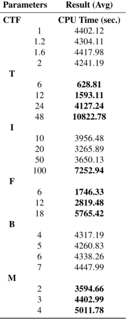
The test instances are solved using IBM ILOG CPLEXTM Optimization Studio 12.5.1. All computational experi-ments have been run on an AMD Phenom II X2 B57 3.20 GHz with 3.24GB of RAM. The relative MIP gap toler-ance is set to 0.5%. A summary of the results can be found in Tables 2 and 3, where the average results of all instances are provided for a given value of each of the parameters CT F, T , I, F, B and M.
Table 2 shows the average solution gap and the average resolution time. The average solution gap is the
percent-age of (U B − LB)/LB. Large CPU Times are observed and rather independently of the variations of most param-eters. A significant increase of the CPU time is observed when the length of the planning period increases. The av-erage CPU Time is multiplied by more than 17 when the number of periods increases from 6 to 48. The CPU Time also significantly increases when the number of Top wafer references increases.
Parameters Result (Avg) CTF CPU Time (sec.)
1 4402.12 1.2 4304.11 1.6 4417.98 2 4241.19 T 6 628.81 12 1593.11 24 4127.24 48 10822.78 I 10 3956.48 20 3265.89 50 3650.13 100 7252.94 F 6 1746.33 12 2819.48 18 5765.42 B 4 4317.19 5 4260.83 6 4338.26 7 4447.99 M 2 3594.66 3 4402.99 4 5011.78 Table 2: Average resolution times
Table 3 shows the percentage of each cost component in the total optimal cost. The percentage of Base Wafer pur-chase and procurement cost is significantly larger than the percentage of the Fresh Wafer purchase and procurement cost. The reason is that less Fresh Wafer procurement is needed as Refresh Wafers are produced using the refresh process. However, since the refresh process is relatively cheaper than Fresh Wafer procurement, relatively small refresh process and setup costs are incurred. The largest production and setup costs are associated to the SOI fab-rication. Inventory costs are negligible for each cost com-ponent even if inventory costs are slightly larger for SOI production.
Except for the length of the planning horizon (T ), the vari-ation of all other parameters do not significantly alter the percentages of the cost components. By increasing the
Parameters Results
Top (Fresh) Wafer Procurement Base Wafer Procurement SOI Production Refresh Process CTF Purchase Procurement Inv. Purchase Procurement Inv. Production Setup Inv. Refresh Setup Neg. Inv.
1 9.36% 0.03% 0.01% 20.43% 0.20% 0.00% 61.30% 1.02% 0.34% 7.07% 0.23% 0.00% 1.2 9.33% 0.03% 0.01% 20.43% 0.21% 0.00% 61.29% 1.04% 0.36% 7.07% 0.23% 0.00% 1.6 9.06% 0.03% 0.01% 20.50% 0.20% 0.00% 61.49% 1.01% 0.34% 7.13% 0.23% 0.00% 2 9.17% 0.03% 0.01% 20.46% 0.21% 0.00% 61.39% 1.03% 0.36% 7.11% 0.24% 0.00% T 6 18.63% 0.06% 0.02% 18.65% 0.18% 0.00% 55.95% 0.92% 0.34% 5.08% 0.16% 0.00% 12 10.17% 0.03% 0.01% 20.28% 0.20% 0.00% 60.83% 1.01% 0.35% 6.89% 0.22% 0.00% 24 5.32% 0.02% 0.01% 21.20% 0.21% 0.00% 63.60% 1.07% 0.37% 7.93% 0.26% 0.00% 48 2.72% 0.01% 0.00% 21.71% 0.22% 0.00% 65.14% 1.08% 0.34% 8.49% 0.28% 0.00% I 10 9.05% 0.05% 0.02% 20.19% 0.31% 0.01% 60.57% 1.54% 0.91% 7.01% 0.35% 0.00% 20 9.33% 0.04% 0.01% 20.37% 0.26% 0.00% 61.11% 1.29% 0.26% 7.05% 0.29% 0.00% 50 9.23% 0.02% 0.00% 20.67% 0.12% 0.00% 62.01% 0.62% 0.00% 7.18% 0.14% 0.00% 100 9.38% 0.01% 0.00% 20.74% 0.06% 0.00% 62.23% 0.31% 0.00% 7.19% 0.07% 0.00% F 6 9.32% 0.04% 0.03% 20.22% 0.27% 0.00% 60.66% 1.35% 0.78% 6.98% 0.33% 0.01% 12 9.18% 0.03% 0.01% 20.45% 0.21% 0.00% 61.36% 1.03% 0.39% 7.10% 0.23% 0.00% 18 9.26% 0.03% 0.01% 20.48% 0.20% 0.00% 61.45% 0.98% 0.27% 7.10% 0.22% 0.00% B 4 9.20% 0.03% 0.01% 20.47% 0.20% 0.00% 61.40% 1.00% 0.35% 7.10% 0.23% 0.00% 5 9.14% 0.03% 0.01% 20.47% 0.21% 0.00% 61.42% 1.03% 0.34% 7.11% 0.23% 0.00% 6 9.30% 0.03% 0.01% 20.44% 0.21% 0.00% 61.32% 1.03% 0.36% 7.08% 0.23% 0.00% 7 9.27% 0.03% 0.01% 20.45% 0.21% 0.00% 61.34% 1.03% 0.34% 7.08% 0.23% 0.00% M 2 9.38% 0.03% 0.01% 20.42% 0.20% 0.00% 61.27% 1.02% 0.37% 7.06% 0.23% 0.00% 3 9.11% 0.03% 0.01% 20.48% 0.20% 0.00% 61.45% 1.02% 0.34% 7.12% 0.23% 0.00% 4 9.20% 0.03% 0.01% 20.46% 0.21% 0.00% 61.39% 1.02% 0.34% 7.10% 0.23% 0.00%
Table 3: Cost components for different data sets
planning horizon, the Fresh Wafer purchase (and also pro-curement and inventory) cost drastically reduces while the refresh process and setup costs increase. Note that the maximum refresh level nmaxf is 5. This means that a newly bought Fresh Wafer can only be refreshed five times. As the lead time is equal to one period (without any SOI and refresh capacity restrictions), it takes 7 periods to fully use a purchased Fresh Wafer. Therefore, as the planning hori-zon increases, the refresh process becomes more impor-tant. Therefore, when the planning horizon increases, the Fresh Wafer procurement cost decreases and the refresh process cost increases. However, as the Fresh Wafer pur-chase cost is relatively larger than the refresh process cost, the decrease of the Fresh Wafer procurement cost com-ponents is larger than the increase of the refresh process cost components. This illustrates the economical impor-tance of the refresh process and that an efficient produc-tion planning contributes to a substantial cost decrease. Note that, as the percentage of the Fresh Wafer procure-ment cost decreases, the Base Wafer procureprocure-ment and SOI production cost percentages increase in the total planning cost.
6 CONCLUSION AND PERSPECTIVES
In this paper, the supply chain of a SOI fabrication unit using the Smart-CutTM Technology was modeled. Using this technology, one of the two purchased raw materials can be used several times after reprocessing. The repro-cessing which is considered as a kind of “remanufactur-ing” can be done internally or externally. A mixed-integer linear programming (MILP) model is proposed to model
the supply chain. The model is validated and the opti-mal solution behavior is studied using generated data sets based on industrial data.
The refresh capacity is constrained by both the refresh line capacity and the SOI production line capacity. In fact, it is the SOI production which determines the rate of the generation of Negatives. Therefore, the refresh process throughput depends on the available refresh capacity and the SOI production (generation of Negatives) rate. Due to the purchase and refresh cost structure, optimal so-lutions in our numerical experiments usually include pur-chase and refresh campaigns, which cause an irregular and fluctuating cost profile along the planning horizon. This may not be desirable both financially and for workforce management, for which a more stable cost expense over the whole planning horizon is preferable. A possible ap-proach is to use a non-linear cost objective function in or-der to make the sum of all costs closer to their average. However, it makes the model non-linear and its resolution much more difficult.
An interesting challenge is to study the properties and characteristics of the proposed MILP model to develop a more effective resolution approach.
Some bulk (namely Fresh Wafer) suppliers also propose to perform the refresh process. Bulk suppliers, being com-petitors, do not allow their products to be handled by another supplier. Therefore, Fresh references which are bought from a supplier must be either refreshed internally or externally only if the same supplier proposes the refresh
MOSIM14 - November 5-7-2014 - Nancy - France
process. This industrial constraint is also to be considered in future studies.
ACKNOWLEDGMENTS
This study has been done within the framework of a joint collaboration between SOITEC (Bernin, France), and the Center of Microelectronics in Provence of the École des Mines de St-Étienne (Gardanne, France). The authors are grateful to the Supply Chain Department of SOITEC for their full support and would like to thank the ANRT (As-sociation Nationale de la Recherche et de la Technologie) which has partially financed this study.
References
Agrali, S. (2011). A Dynamic Uncapacitated Lot-Sizing Problem with Co-Production, Optimization Letters 6(6): 1051–1061.
Billington, P. J., McClain, J. O. & Thomas, L. J. (1983). Mathematical Programming Approaches to Capacity-Constrained MRP Systems: Review, For-mulation and Problem Reduction, Management Sci-ence29(10): 1126–1141.
Brahimi, N., Dauzère-Pérès, S., Najid, N. M. & Nordli, A. (2006). Single Item Lot Sizing Problems, European Journal of Operational Research168(1): 1–16. Bruel, M. (1995). Silicon on Insulator Material
Technol-ogy, Electronics Letters 31(14): 1201–1202. Ferrer, G. & Whybark, D. C. (2001). Material Planning
for a Remanufacturing Facility, Production and Op-erations Management10(2): 112–124.
Helber, S. & Sahling, F. (2010). A Fix-and-Optimize Ap-proach for the Multi-Level Capacitated Lot Sizing Problem, International Journal of Production Eco-nomics123(2): 247–256.
Helmrich, M. J. R., Jans, R., van den Heuvel, W. & Wagel-mans, A. P. (2014). Economic Lot-Sizing with Re-manufacturing: Complexity and Efficient Formula-tions, IIE Transactions 46(1): 67–86.
Karimi, B., Fatemi Ghomi, S. & Wilson, J. (2003). The Capacitated Lot Sizing Problem: A Review of Mod-els and Algorithms, Omega 31(5): 365–378. Kenné, J.-P., Dejax, P. & Gharbi, A. (2012).
Pro-duction Planning of a Hybrid Manufacturing-Remanufacturing System under Uncertainty within a Closed-Loop Supply Chain, International Journal of Production Economics135(1): 81–93.
Soitec, W. (2014). Soitec Smart Cut Technology. Spengler, T., Puechert, H., Penkuhn, T. & Rentz, O.
(1997). Environmental Integrated Production and Recycling Management, European Journal of Oper-ational Research97(2): 308–326.
Tomlin, B. & Wang, Y. (2008). Pricing and Opera-tional Recourse in Coproduction Systems, Manage-ment Science54(3): 522–537.
Trigeiro, W. W., Thomas, L. J. & McClain, J. O. (1989). Capacitated Lot Sizing with Setup Times, Manage-ment Science35(3): 353–366.
Zhang, Z.-H., Jiang, H. & Pan, X. (2012). A La-grangian Relaxation Based Approach for the Ca-pacitated Lot Sizing Problem in Closed-Loop Sup-ply Chain, International Journal of Production Eco-nomics140(1): 249–255.