3D reconstruction of a catheter path from a single view X-ray sequence

iÏ/’ 36g .

/

Université de Montréal

3D reconstruction of a catheter path

from a single view X-ray sequence

par

Ji

Yao Weng

Département d’informatique et de recherche opérationnelle Faculté des arts et des sciences

Mémoire présenté à la faculté des études supérieures En vue de l’obtention du grade de

Maître ès sciences (M.Sc.) en informatique

août 2003 © Ji Yao Weng, 2003

t3

q,

()L3

Université

(Hi

de Montréal

Direction des bibliothèques

AVIS

L’auteur a autorisé l’Université de Montréal à reproduire et diffuser, en totalité ou en partie, par quelque moyen que ce soit et sur quelque support que ce soit, et exclusivement à des fins non lucratives d’enseignement et de recherche, des copies de ce mémoire ou de cette thèse.

L’auteur et les coauteurs le cas échéant conservent la propriété du droit d’auteur et des droits moraux qui protègent ce document. Ni la thèse ou le mémoire, ni des extraits substantiels de ce document, ne doivent être imprimés ou autrement reproduits sans l’autorisation de l’auteur.

Afin de se conformer à la Loi canadienne sur la protection des renseignements personnels, quelques formulaires secondaires, coordonnées ou signatures intégrées au texte ont pu être enlevés de ce document. Bien que cela ait pu affecter la pagination, il n’y a aucun contenu manquant.

NOTICE

The author of this thesis or dissertation has granted a nonexclusive license allowing Université de Montréal to reptoduce and publish the document, in part or in whole, and in any format, solely for noncommercial educational and research purposes.

The author and co-authors if applicable retain copyright ownership and moral rights in this document. Neither the whole thesis or dissertation, nor substantial extracts from it, may be printed or otherwise reproduced without the author’s permission.

In compliance with the Canadian Privacy Act some supporting forms, contact information or signatures may have been removed from the document. Whi)e this may affect the document page count, it does not represent any loss of content from the document.

Faculté des études supérieures

Ce mémoire de maîtrise intitulé

3D reconstruction of a catheter path

from a single view X-ray sequence

Présenté par Ji Yao Weng

A été évalué par un jury composé des personnes suivantes:

Dr. Sébastien Roy Président-rapporteur Dr. Jean Meunier Directeur de recherche Dr. Pierre Poulin Membre du jury

111

$ ommaire

Plus de 1/3 des décès enregistrés au Canada au cours des dernières années sont causés par les maladies cardiovasculaires. L’un des problèmes cardiovasculaires le plus communs est l’athérosclérose coronaire qui consiste en l’accumulation de plaques sur les parois des artères. La recherche sur les niveaux de risque de l’athérosclérose coronaire est, par conséquent, de très grande importance pour le diagnostic et ta stratégie thérapeutique à entreprendre ultérieurement. Cliniquement, l’imagerie IVUS (ultrasons intravasculaires) combinée avec l’angiographie est largement utilisée pour l’examen médical et le traitement des maladies cardiovasculaires.

Dans l’imagerie IVUS, les méthodes « pose estimation » sont employées pour déterminer la trajectoire du cathéter à partir d’une projection unique obtenue par angiographie. Des progrès remarquables ont été réalisés par les travaux de recherche sur la «pose estimation», à partir d’une vue _{unique en image, et par l’implémentation de}

méthodes de reconstruction 3D de la trajectoire du cathéter dans une imagerie IVUS. En dépit de ces améliorations significatives, l’exigence d’une connaissance antérieure de la configuration 3D des artères coronaires est un inconvénient majeur qui se pose lors de la construction 3D de la trajectoire du cathéter dans une imagerie IVUS. Malheureusement,

il y a eu un manque d’exploration de nouvelles méthodes susceptibles de pallier cet

inconvénient.

Cette thèse se focalise sur la «pose estimation» à partir d’une projection unique et ce, pour une reconstruction 3D de la trajectoire du cathéter dans une investigation IVUS. Premièrement, nous explorons l’état de l’art de la «pose estimation» projection unique en passant en revue et en simulant trois méthodes typiques choisies parmi d’autres. Les inconvénients des méthodes existantes nous ont motivés à étudier la possibilité d’une «pose estimation» à partir d’une séquence d’images. Nous proposons une nouvelle méthode de pose estimation à partir d’une séquence d’images de vue unique

visant la reconstruction du la trajectoire de cathéter dans imagerie IVUS. Ensuite, nous simulons avec un logiciel mathématique la méthode proposée par des courbes spirales et nous l’appliquons par la suite à une séquence d’images obtenues à partir d’une expérimentation fantôme. Les résultats obtenus montrent que les erreurs de reconstruction varient entre 5.81% et 6.68% pour les simulations et 1.25% à 1.36% (en termes de taille de fantôme reconstruit) pour l’étude fantôme.

Bien que ces chiffres pourraient sembler plutôt médiocres, ils sont réellement une mine d’or pour les médecins qui n’ont pas accès aux informations 3D (à moins d’utiliser un laboratoire complexe proposé par une autre méthodologie, ce qui est impraticable dans les cliniques). La méthode proposée a l’avantage, d’une part, d’une installation beaucoup plus facile dans les cliniques et, d’autre part, d’un coût inférieur à celui des méthodes existantes d’autant plus qu’elle conduira certainement, à l’avenir, à un outil de valeur.

V

Abstract

Cardiovascular disease causes over 1/3 of ail deaths in Canada in recent years. One of the most common cardiovascular problems is coronary atherosclerosis, the build up of plaque on artery walls. The investigation of the severity of coronary atherosclerosis is therefore very important for the diagnosis and therapeutic strategy that will be undertaken. Clinically, IVUS (Intravascular Uttrasound) imaging combined with angiography is widely used in examination and treatment of cardiovascular diseases.

In IVUS imaging, methods of pose estimation are used to determine the trajectory of the catheter from single projection images obtained by angiography. The research on pose estimation from single view images or one single view image bas achieved remarkable progress, and methods have been implemented in the 3D reconstruction of catheter trajectory in IVUS imaging. Despite these significant improvements, the requirement of previous knowledge of the 3D configuration of the coronary arteries is a significant drawback that stili exists in the implementation of 3D construction of a catheter trajectory in IVUS imaging. Unfortunately, there lias been a lack of exploration ofnew metbods that could overcome this drawback.

This thesis focuses on pose estimation from single projection aiming to the 3D reconstruction of the catheter trajectory in an IVUS investigation. Firstly, we investigate the state ofart of pose estimation by single projection by reviewing and simulating three typical methods, which are cliosen from a variety of published papers reÏated to the topic. The drawbacks of existing methods motivate us to investigate the possibility of pose estimation from an image sequence. We propose a novel method of pose estimation from a single view image sequence targeted for the reconstruction of the catheter trajectory in IVUS imaging. Afterward, we simulate the proposed method with spiral curves in the Mathematica® environment, and apply the proposed method to an image sequence obtained from a phantom experiment. Typical resuits show reconstruction errors ranging from 5.81% to 6.68% for the simulations and 1.25% to 1.36% (in terms ofthe size oftbe

reconstructed phantom) for the pliantom study. Aithough these figures could seem rather mediocre, they are actualiy a goid mine for the physician that lias access to no 3D information at ail in clinic today (unless he uses quite complex “laboratory” set-up proposed by other methodologies, which is unfeasibie in clinical practice). The proposed method has advantages of much easier set-up in the clinical environment and lower cost than existing methods, thus it will certainly lead to a vaiuable tool in the future.

vii

Table of Contents

Chapter 1 Introduction

-

1

-1.1 Introduction - 1

-1.2 Pose Estimation in Intravascular Ultrasound Modality -4

-1.3 Motivation -4

-1.4 Organization of the Thesis - 5

-Chapter 2 E xisting Pose Estimation Methods - 7

-2.1 Introduction - 7

-2.2 The Problem of Pose Estimation by Single Projection - 10 -2.3 Review of Three Methods of Pose Estimation by Single Projection - 12

-2.3.2 SPI Method - 14

-2.3.3POSIIMethod

-19-2.4 Comparison of the Three Methods - 22

-2.5 Summary - 3$

-Chapter

3 A

Method of

Pose Estimation by an Image Sequence

from Single Projection -

39

-3.1 Introduction - 39

-3.2 Angïography in IVUS intervention -40

-3.3 A Method of Pose Estimation with an image Sequence from Single Projection-41

-3.3.1 A Geometrical Analysis ofthe Problem of Pose Estimation by an Image

Sequence from Single Projection -41

-3.3.2 Finding Solutions for a Trajectory Curve -44

-3.3.3 Determination ofthe right solution from multiple solutions - 46 -This section discusses how to choose the right solution from multi-solutions

obtained in the last subsection. We first project the points of each possible solution onto the image plane using the following equations - 46

-3.3.4 Reducing Accumulated Error -46

-3.3.6 A Summary ofProposed Method - 48

-3.4 Simulation of Proposed Method in Mathematica - 51

-3.4.1 Simulations basedonknown Z1 - 53

-3.4.2 A Simulation for the determination of Z1 - 57

-3.5 Summary - 57

-Chapter 4 Application of the Proposed Method to Synthetic Data...

- 59

-4.2 Phantom Experiment.- 59 -4.3 Application of the Proposed Method on the Phantom Experiment Data....- 63 -4.3.1 Application ofthe Proposed Method on Image Sequence I - 63 -4.3.2 Application ofthe Proposed Method on the Image Sequence II - 65

-4.4 Summary - 66

-Chapter 5 Conclusion

—

69

— 5.1 Conclusion - 69 -5.2 Summary of Contributions - 70 -5.3 Future Research - 70

-References

-

72

-ix

List of Tables

Table 2.1 _{Within a small rotation around the Z-axis, Newton’s method, SPT} method, and POSIT obtain proper solutions. SPI demonstrates a good performance in terms of accuracy, while P0511 demonstrates a good

performance in terms of efficiency - 24

-Table 2.2 _{Within a small rotation around the Z-axis, Newton’s method, SPI} method and P0511 obtain proper solutions. POSIT demonstrates good

performances in terms of accuracy and efflciency - 25

-Table 2.3 _{With this test data, both Newton’s method and SPI method cannot}

obtain a proper solution - 26

-Table 2.4 The same test data as in -Table 6.1(d), but a proper set of initial estimates of rotation angles are given, SPI obtains a proper solution, while

Newton’s method stili fails to find the solution - 27

-Table 2.5 With this test data, Newton’s method fails to find the solution. P0511

method demonstrates better performance in terms of efficiency and accuracy.. . .-28

-Table 2.6 With this test data, Newton’s method failed to find the solution. The P0511 method demonstrates better performance in terms of efficiency and

accuracy - 29

-Table 2.7 With the test data, Newton’s method failed to find the solution. The POSIT method demonstrates better performance in terms of efficiency and

accuracy - 30

-Table 3.1 Simulation ofthe proposed method whenr = 100, h = 32 andAt = 0.3. ..- 54-Table 3.2 Simulation ofthe proposed method whenr = 100, h = 32 andAt = 0.2. ..- 55

-Table 3.3 Simulation ofthe proposed method when r 50, h = 16 andAt 0.25. ..- 56-Table 3.4 In the first iteration, Zj is roughly estimated between 520 and 540 - 57

-Table 3.5 In the second iteration, Z1 is estimated as 530 - 57

-Table 4.1 _{The Image Sequence I, which is obtained from the original sequence}

with an interval of 45 frames - 64

-Table 4.2 The trail ofProcedure Find_Zi in the range of838mm to 908mm - 64

-Table 4.3 The Image Sequence II, which is obtained from the original sequence

with an interval of 52 frames - 66

-66-List of Figures

Figure 1.1 A single frame ofIVUS image _-2

-figure 1.2 Angiograms (left) and two IVUS images taken from the sequencc (riglit) with the corresponding 3-D reconstruction (middle). (ref: Whale et al. http://www.engineering.uiowa.edu/ —awahle/WahIUS/Slides/virtual

angioscopy.pdf)

- 3

-Figure 2.1 _{Geometry of pose estimation by single projection problem. The model} points in the camera reference frame and the model reference frame are denoted by (X Y, Z) and (Xtm, yE,

Ztm), respectively. The image ofa model

point on the image plane is denoted as (xAl,,M)

- 10

-figure 2. 2 Projection ofa point P onto the image plane at [x1, y1f, and the

corresponding measured image coordinates at [x’ ),M ]T

-5

-Figure 2.3 The point positions, P, are projected onto their repective perspective

projection une, from the focal spot to the [x,y_{j’, at the positions P”} - 16

-figure 2.4 Scheme ofthe POSIT method. The image p is the perspective

projection of object point P and imagep°° is the scaled orthographic project

(SOP) ofthe object point P. K is the plane through Po and parallel to the

image plane - 20

-Figure 3.1 _{The configuration of a system of IVUS combined with coronary} angiography

- 41

-Figure 3.2 A segment of trajectory ofa catheter tip and its projection on the image

plane

-43-Figure 3.3 11 is the plane that passes through the point P1+j and is parallel to the X and Y-axis,

_Ø

_{is the angle between the une ofP1P+1 and the plane n} -43

-Figure 3.4 The error analysis ofthe week perspective project vs. the full

perspective project - 47

-figure 4.1 _{The phantom is built with a l000nzl beaker with a pipe spiraling on it}

about 360°. The measurernent for h and d are: h= 125m,,, and d=lO9mm - 60

-Figure 4.2 The measurements ofthe pipe: e =3.176mm andt= 6.35mm - 60

-xi Figure 4.4 The configuration ofthe fluoroscopic camera system in the phantom

experiment -62

-Figure 4.5 A frame ofthe fluoroscopic image sequence. The transducer along the catheter is visible in the lower left quadrant ofthe image. The circular object appearing along the tube are simply twist tights attached at regular intervals

-Acknowledgements

First and forernost, I would like to thank my supervisor, Dr. Jean Meunier, for providing me the opportunity to work on this thesis project. His insight, valuable advice and guidance throughout my work have contributed significantly to this research. Also, I would like to express my appreciation to Dr. Jean Meunier for his financial support.

I would like to thank the Montreal Heart Tnstitute for providing the data of a phantom experiment for my thesis project work. I also would like to thank Mr. Denis Sherknies for his preparation of the documents for the experimentat data.

I am very gratefiil to my wife, Man, and my son, Yi Ran, for their love and sacrifices, and for providing me encouragement and inspiration during my graduate study.

1

Chapter 1

Introduction

1.1 Introduction

Among ail pathologies affecting the modem world, cardiovascular diseases are at the forefront. In Canada, they account for the death of more Canadians than any other disease. In 1999 according to Statistics Canada, cardiovascular diseases killed 78,942 Canadians, 36% of ail deaths in Canada. They cost Canadian economy over $18 billion a year according to a 1994 study by the Heart and Stroke Foundation. One of the most common cardiovascular problems is coronary atherosclerosis, the buiÏd up of plaque ta combination of cholesterol, cellular waste, and other materials) on artery walls. Plaque can cause a heart attack by severely reducing or stopping the blood flow through a coronary artery. Moreover, the plaque can rupture and form bÏood dots capable of blocking arteries. The investigation ofthe severity of coronary atherosclerosis is therefore very important for the diagnosis and therapeutic strategy, such as medication, bypass surgery, angioplasty (dilation) with or without stent, which will be undertaken. For this purpose, two main imaging methods are used nowadays. Angiography (X-rays) consists of the injection with a catheter of a contrast product in the lumen of the arteries, making them opaque to X-rays. Using several views (projections) the physician can get an assessment of the position and geometrical severity of the stenosis (narrowing of the artery due to atherosclerosis). It is nevertheless important to remember that a single angiogram reveals only a 2-D “silhouette” of the tme 3-D lumen. This has for consequence that an image under only one (or even a few) angle of sight can badly represent the extent of a complex stenosis. Although 3-D reconstruction atgorithms exist in angiography based on two or more views, it remains that angiography visualizes only the inner lumen of the vessel and cannot determine directly if the vessel wall has

atherosclerosis; for instance it could miss diffuse (long) lesions with seemingly no stenosis. Intravascular ultrasound (IVUS) represents a complement (even an alternative) to angiography for the direct visualization of the arterial anatomy. A miniaturized ultrasonic transducer at the end of a catheter is inserted in the artery lumen and brought beyond the lesion of interest and then withdrawn gradually, manually or automatically. Contrary to angiography, which represents a silhouette of the arterial lumen, IVUS produces unique echographic images (Figure 1.1) showing the cross-section of coronary arteries. These images reveal clearly the lumen, watls and plaque, and offer a powerful tool for diagnostic purposes. Unfortunately, this sequence of images does not offer direct information about the 3-D geometry of the artery, an essential feature to reliably compute plaque volume or sheer stress.

Athero. Plaque Catheter Lumen Intima Media

figure _{1.1 A single frame ofWUS image.}

Because there is no information about the 3-D location and orientation associated with each frame of an IVUS image sequence while coronary angiography can be used to localize and even to reconstruct of coronary arteries in 3-D, IVUS and angiography together are widely utilized in assessment of coronary artery diseases in cÏinics (Figure

3

In a typical IVUS intervention, a few single projection angiographic sequences are taken to localize the WUS transducer dunng its pullback. In addition, the pullback length can be measured. This implies that it could be possible to obtain the reconstruction of coronary arteries. The task of this research is to develop a novel pose estimation method in which an image sequence from one single projection is used to obtain the reconstruction of coronary arteries, instead of using a two-camera system such as in biplane angiography or additional CI or MR information in single projection angiography. As a result, the costs of clinical equipment and clinical processing could be reduced for reliable 3-D artery measurements.

figure 1.2 _{Angiograms (left) and two WUS images taken from the sequence (right) with the} corresponding 3-D reconstruction (middle). (ref: Whale et al. http://www.engineering.uiowa.edu! -awahle/WahHJS/Slides/virtual-angioscopy.pdf).

1.2 Pose Estimation in Intravascular Ultrasound Modality

Pose estimation is a method for determining the location and orientation of a 3-D object with respect to a camera system from 3-D to 2-D point correspondences. Two kinds of pose estimation methods are used in angiography: biplane angiography [1, 2], in which images from two views are needed, and single projection angiography [3, 4, 5, 6,

10, 11, 14], in which only one view image and prior knowledge of 3-D configuration of

the object are required. Research on biplane pose estimation has achieved significant progress. Unfortunately, the required biplane angiography system is more expensive, usually takes more physical space, and is much more complex to operate than single projection angiography. This partly explains why these systems are not available everywhere and even tend to disappear from clinical practice.

Pose estimation from single view needs a previous knowledge of the 3-D configuration of the object. In single projection angiography implementation, this knowledge of 3-D configuration of coronary arteries can be obtained by either computed tomography (CT) or magnetic resonance (MR). This requirement of an extra clinical processing is a drawback of single projection angiography. Pose estimation from single view has more challenges than biplane pose estimation due to its specific difficulties.

In this thesis we focus on pose estimation with a single angiographic projection with knowledge limited to the pullback distance traveled by the ultrasonic transducer in IVUS intervention.

1.3 Motivation

So far, researchers have focused on implementation of model-based pose estimation in single plane angiography ignoring the information that could be obtained in the specific situation of an IVUS intervention. In a practical clinical situation, an image sequence can 5e taken from single projection during pullback of the catheter during the IVUS _{intervention, and the pullback length of catheter in the interval between two} successive images can be measured. Based on this specific situation in IVUS intervention, a novel method is proposed in this thesis to reconstruct the trajectory ofthe catheter tip. This trajectory represents the 3-D pose of the catheter that is estimated from

5

the 2-D projection on the image sequence.

The proposed pose estimation method overcomes the main drawbacks of biplane pose estimation methods and model-based single project pose estimation methods by reducing the clinical costs. Compared with biplane pose estimation and model-based pose estimation, the estimation of pose from a single plane angiography image sequence and the measurement to pullback length is rather difficuit. A significant challenge is that, mathematically, there exist multiple pose solutions corresponding to a given image sequence with known pullback measurements, but there is no geometrical condition that can be used to determine the right solution from the multiple solutions. To solve this problem, we consider the physical characteristics of a catheter and assume that there is no sharp bend of the catheter.

In terms of accuracy, efficiency, and stability, the proposed method is not as good

as the existing pose estimation methods. However, considering its much easier setup in

the clinicaÏ environment the proposed method will certainly leaU to a valuable tool in the future.

1.4 Organization of the Thesis

This thesis presents a study on pose estimation by single projection in the context of IVUS intervention. The thesis is organized as follows.

In Chapter 2, we begin with the definition of pose estimation from single projection. Then we review and simulate three typical methods of pose estimation chosen from various existing methods. These three typical methods are Newton’s method, a classic method, SPT, a method developed intendedly for angiography implementation, and POSIT, a recently published method. The simulation resuits on several cases, and a comparison in terms of accuracy, efficiency, and stability are presented. In Chapter 3, we analyze the problem of pose estimation with a single plane image sequence and a measurement of the catheter pullback length, and the difficulties associated with this problem. To solve the problem, we propose a new method, which is presented in detail. Furthermore, the proposed method is simulated using several given cases and the simulation results are shown. In Chapter 4, the proposed method is applied to phantom (physical model) image sequences provided by the Montreal Heart. Chapter 5 concludes

the thesis by highlighting the findings of this investigation and by suggesting some possible future work.

7

Chapter 2

Existing Pose Estimation Methods

2.1 Introduction

Conventional 3-D IVUS uses an automated puÏïback device to get a stack of IVUS images providing additional information for volumetric measurements. Unfortunately this rnethod assumes a straight vessel, which is a crude approximation for coronary arteries. In fact, due to the vesse! cuwature, the image planes are flot parallel. Moreover the catheter twists when following a tortuous vesse! generating a rotation artifact in the image plane. Thesc problems must be considered to compute a truc 3-D reconstruction of the vesse! from IVUS images. A few groups [1, 2] have successfully implemented solutions to this problem using biplane angiography to infer the 3-D trajectory ofthe catheter. At the University of Iowa [1], they extract the 2-D catheter path in both biplane angiograms and then reconstruct the 3-D trajectory knowing the biplane imaging system geometry. Assuming a known constant pullback speed, the actual location of each IVUS frame along (and perpendicular to) the 3-D pullback path is obtained. b _{compute the catheter twist, they determine the relative rotation with a} sequential triangulation method and the absolute orientation from the out-of-center position of the IVUS catheter used as a landmark in both angiograms and IVUS images. Another group [2] from the Cleveland Clinic Foundation has proposed a method that could be used with or without a pullback device. The 3-D trajectory of the IVUS transducer was computed as a function of time using biplane angiography similarly to the University of Iowa’s group. Each IVUS frame was time-synchronized with the angiographic images and then correctly positioned perpendicular to the trajectory. Then,

a 3-D segmentation method based on a 3-D extension of active contours (snakes) extracts

the best twist. Unfortunately, the required biplane angiography system is more expensive, usually takes more physicai space, and is much more complex to operate than its single plane parent. This partly explains why these systems are not available everywhere and even tend to disappear from clinicai practice. In addition, for IVUS arteryreconstruction,

a calibration step (to assess the biplane imaging system geometry) is necessary and the X

ray radiation dose to the patient could typically be higher. Ail this would add a significant burden to the already quite complex IVUS intervention protocol. We believe that atthough the biplane approach gives spectacular results it will probably find limited use

in clinical practice except in university hospital research laboratories. As for the use of

3-D position sensors (e.g., _{six-degree-of-freedom magnetic sensor) for tracking the}

trajectory of the transducer, this is indeed an efficient method for 3-D conventional ultrasound transducer but this is certainly a big technological challenge for IVUS and is probably not reachable in the near future.

Because of the drawbacks existing in biplane angiography for IVUS artery

reconstruction, there has been a rise of implementations of single projection angiography for IVUS artery reconstruction [4, 5, 11]. It overcornes the drawbacks existing in biplane angiography.

In this thesis, we focus on pose estimation from single projection methods, which are employed in single projection angiography. The rest of this chapter presents a review and simulations of three typical pose estimation methods that are chosen from many publications in the computer vision community and biomedical engineering community. These methods are Newtons method [3], SPT (Single Projection Technique) by Hoffman

et al. [4, 5, 11], and POSIT (Pose from Orthography and Scaling with ileration) by

Demonthon et al. [6, 14]. In the next chapter, we will present our research on pose estimation by image sequence from single projection.

Newton’s method is named after Newton’s numerical method that is empioyed to solve systems of nonlinear equations, which are obtained from the relation of object points and their corresponding full perspective projections. Newton’s method is simple and straightforward. The main drawback of Newton’s method is that it has a Iimited suitable scope of location and orientation for the object.

9

angiography modality. The main idea of SPT is to align the object points with their corresponding projections by adjusting translation and rotation using projection Procmstes technique [7, 8, 9]. The method lias two main steps. The first step is to align the object points with their corresponding projections by adjusting the translation in the x-y plane iteratively. In the second step, projection-Procrustes technique is carried out to adjust the translation and rotation to optimize the alignment ofthe object points with their corresponding projections. SPI is tested in a phantom experiment by Hoffman et al., and the resuits are given in [5]. However, the phantom experiment is based on several dots that are fixed in a known configuration instead of a catheter. SPI is relatively complex. In terms of stability, SPI is better than Newton’s method, but stiit lias the drawback of a limited suitable scope of location and orientation for the object.

POSIT emerged recently. It consists of iteratively improving the pose computed with weak perspective projection (i.e., _{scaled orthographic projection) camera model to}

converge to a pose estimation computed with a perspective projection camera model. Furthermore, Horaud et al. [14] derive the idea for POSIT and develop an improved version of POSIT by using paraperspective projection instead of weak perspective projection. According to our simulation in Mathematica, POSIT is the best method for pose estimation by single projection in terms of efficiency, accuracy, and stability among the three methods.

This chapter is organized as follows: Section 2 gives a geometrical definition for the problem of pose estimation from single projection. Section 3 reviews the Newton’s method, the SPI method, and the POSII method. A modification that we have made to reduce the slow convergence problem existing in SPI is also described in Section 3. In Section 4, a comparison among the three methods based on the simulation resuits is presented. Section 5 presents a summary for this chapter.

2.2 The Problem of Pose Estimation by Single Projection

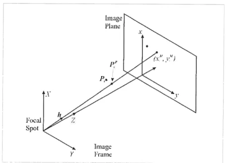
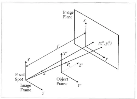
Pose estimation by single projection is also called rnodel-based pose estimation, or mode! matching, or optical jigging. The geometry of pose estimation by single projection

is depicted in Figure 2.1. The 3-D camera coordinate system, (X Y, Z), is defined such

that its origin is located at the focal spot. The image plane is located at a distance of focal length,

_f

_{from the focal spot, and the image coordinate system, (x, y), lying in the image} plane, is parallel to X and Y. The superscript M in (xM, _{y’) is used to denote measured}

image coordinates. Independent of the camera reference frame, the 3-D model coordinate system, (Xv, Y’, Ztm), is defined relative to the points in the object itself. The pose estimation by single projection problem can be stated as follows:

- Let P1m, ..., Pm, with P”’ =[X’1, ,Z[’

]T

and n 3, expressed in the model

reference frame, ben points of an object mode!.

- Let P1, ..., P4,, withP, = [X1, Y,Z.]’, expressed in the camera reference frame,

Image Plane Spot lnmge Fraine frame Y

Figure 2.1 _{Geometry of pose estimation by sing!e projection problem. The mode! points in the}

camera reference frame and the model reference frame are dcnoted by (X Y, Z) and (X’1, Y’1, Z’1),

respectively. The image ofa moUd point on thcimage plane is denoted as (x”,yM)

11

- Let pi,

..., p,,, with p. =[x1,y1

j7,

be the n image points, expressed in the image reference frame, projections oftheP.

The goal is to determine the rigid transformation, i.e., rotation matrix R and translation vector T, aligning the camera reference frame and model reference frame:

1 =R1m +T.

The above equation can be written as

[X1,Y,,Z1]T =R[J(”,Y”,Z”jT +T, (2.1)

where T_{can be represented by T1, T2 and T3, the translations along the X Y, and Zaxes,} as follows:

T=[T,T,,T3]T, (2.2)

and R can be represented by Euler angles,

_Ø,,

ç and q, the rotation angles about the Y andZaxes ofthe camera reference frame as in the foltowing equation:

cos

_Ø.

—sin

Ø.

O cos

Ø,

O sin

Ø,

1 0 0

RT = sinØ. cosç& 0 0 1 0 0 cosç5 —sinØ . (2.3) O O Ï —

5m

Ø,

O cos

Ø,

O sin

Ø,

cos

Inversely, Euler angles,

_Ø,

ç5 and _02, can also be computed from R by Euler angle decomposition:

if r31 ±1:

_______

(2.4)

if (r3

)

=

withRbeing written as:

(2.5) = ArcSiJ ________ I 1_(rj)2

J

= ArcSin(r31) 1l = ArcSiJ 1_(,)2

J

=0 = ArcSin(—r,3), R= ‘21

In the equations (2.4), we assume that OØ<180,

2.3 Review of Tliree Methods of Pose Estimation by Single Projection

In this section, we review three typical methods of pose estimation by single projection [3, 4, 5, 6, 10, 11, 14], which are chosen from many publications in the computer vision community and the biomedical engineering community. The methods are Newton’s method, a classic method, SPT method, a method intended for implementation in angiography, and POSIT, a method that emerged recently.

2.3.1 Newton’s Method

The algorithm employs Newton’s iterative method to solve the system of nonlinear equations, which are obtained from the full perspective projection [3].

The relation between object points and their corresponding image points in camera coordinates is given by the full perspective projection equation:

[x1,y1]’

[ixi]T

(2.6)

Ptugging equations (2.1), (2.2), and (2.5) into equation (2.6), we can see that each image point correspondence generates twonon-linear equations,

= ,1X7’ +_I2 +i3Z +] in rn ni i3X1 _+‘32g + i33Z1 + (2 7) — . r, X” +i,)Ç. +,73Z1 +T, in m rn î31X1 +r37Y, +r33Z1 +I

The unknown components of R and T can be determined from a sufficient number of correspondences, each bringing two equations like equation (2.7). The resulting systems have six unknowns,

_{Ø, Ø,, Ø.}

Tj, T,, and T3. Here R depends only on three free parameters ç1,

_Ø1,,

and

_Ø.

Newton’s numerical method is now employed to solve the systems. Assuming that

(, i)

is the tnie solution for the system, the method starts off with an initial guess for and

,

say R° and 1, and computes p through equation (2.7) with R = _{R’ and T=} (k=O, 1,

_...),

until the residuals

5x1 =x1(Rk,TJo)_

(2.8) Sy1 =y1(Rk,Tk)_jY

13

are srnall enough. In equation (2.8), and j5 _{are x andy coordinates ofmeasured image}

points. The first-order expansions of residuals are

-AT+ j=1,2,3 k=x,y,z (2 9) + øk = j=L,2,3 _j k=x,v,z øk

where the partial derivatives with respect to T1, T2, and T3 are

— r ax, — —

f

X aiz’ai ‘ai z.2 and a0 aj a, ai ‘aT,Z1’aT3 zi2.

The partial derivatives with respect to the rotation angles are

— — xj ax, — 2 +Z,2 a, — r, - ‘ -

f

‘ and ay, — )Ç2+z12 ay,

f

XY. X.

f

,2 ‘,• - ‘

-The six unknowns A1, AT,, AI, AØ, AØ,, and AØ in equation (2.9) can be

determined if at least three point correspondences are known. In the iterative process,R and Tare updated as follows:

(2.10) and

(2.11) where Tprev and R‘“

are the values of T and R in the previous iteration, and A T and

AR are the corrections of T and R, respectively. AR _{is calculated with AØ, AØ,,,}

and AØ.. through equation (2.3).

The algorithm ofNewton’s rnethod is sumrnarized as follows:

The input is formed by n _{corresponding image and mode! points, with n 3, and}

1) Using the current estimates of kand , compute Pthrough equation (2.1). 2) ProjectP1onto the image plane through equation (2.6).

3) Compute the residuals & and ‘5y. (j= l,2,...,n).

4) Solve the linear system of n _{instances of equation (2.9) for the unknown}

corrections, AT, AT7, AI, AØ, AØ,, and AØ.

5) _{Update the current estimates of the translation vector T and rotation matrix R.}

6) If the residuals are sufficiently small, exit; else go to step 1.

2.3.2 SPT Method

SPT (Single Projection Technique) [4, 5, 11] lias been developed by Esthappan and

Huffrnann for impternenting the orthogonal Procrustes algorithrn [7, 8, 9]. The process of the rnethod is composed oftwo parts described as follows:

The first part ofthe method uses the differences between the projected model points

(x1 ,y1) and the measured image points (x”,y) _{through the following equations to}

adjust T1 and T2 iteratively.

T TP

[[

_{_ii}}

= T,pv

1

(2.12)

where prev_and TPt(w_{correspond to previous estimates ofT1 and T2, respectively and n is}

the number of points in the model. Figure 2.2 shows the relation between (x ,y.) and

M M

(x1 ,y1

_).

In the second part of the method, R and T are optimized in an iterative manner by using the projection-Procrustes technique. Carrying out of the projection-Procrustes technique involves alignment of the point in the model with their respective projection unes, i.e.,_{the ray trace from the origin, or the focal spot, ofthe camera reference frame to}

15

h—

tx,’,y’,f] - (x)2 +(y’)2

_+f2

Plane Focal Spot Iniagc Y Frame

Figure 2. 2 Projection of a point P onto the image plane at [x1, y]T

and the corresponding

mcasured image coordinates at [x’,y’

]

T

FirstLy, the point positions, P1, are projected onto their respective projection unes, forming_{the corresponding points, P,; sec Figure 2.3. P1 are gÏven by:}

=

hh,

where

(2.13)

(2.14)

is a unit vector directed from the focal spot to p’ = (x’,y’), the measured image

coordinates of the i-th point. The positions of the model points, P, are related to the points on their respective projection lines, P1’, in the camera reference frame according to the following equation:

P”=sPA+r+E (2.15)

where P and P1’ are n x 3 matrices representing the position of the moUd points in the camera reference frame and on the projection unes, respectively, A is a 3x3 rotation matrix, r is a 1 x 3 vector representing the translation from the centroid of P to the centroid of P1’, s _{is a scalar, and E is an n x 3 residual matrix. Equation (2.15) can be}

rewritten as

E=(P1’ —r)—sPA. _(2.16)

Note that for some unknown reasons, our simulation shows that convergence of SPT was unacceptably slow which is different from the resuit given in [5]. We have made

a modification to the formula given in [5] according to the Procrustes algorithm presented

in [7, 8, 9]. We define a new coordinate system, named modeiC, such that its origin is located at the centroid ofP. Then we use pC and [pP]C to represent P and P’ in the modeiC reference frame, and use pC

and [pP]C to replace P and P” —r in equation (2.15), respectively. The translation from camera reference frame to the modelC reference frame is denoted as Ii’. _{In the modeÏC reference frame, the equation (2.15) is rewritten as}

E=tP]c’_sPcA. _(2.17)

In [5], r is flot considered explicitly in the process of projection-Procntstes and the translation I _{is flot mentioned. Afier the modification above, the process can converge} to the solution as expected.

Image Plauc Pi, F. Spot Y Image Iranie

Figure 2.3 The point positions, P, _{are projected onto their rcpectivc perspective projection une,} from the focal spot to the {x1Al M1T,

17

The Procrustes algorithm [7, 8, 9] is used to determine the transformation (i.e., A and s) that aligns pC

and [pP]C

optimally, i.e., sucli that the transformation minimizes the sums of squares of E, given by

Tr(ET .E), (2.18)

In equation (2.18), Tr(A) = is called the trace of square matrixA. The solution for

A is computed by using the orthogonal Procrustes algorithm according to the equation:

A=UVT, (2.19)

where

[pC]T[pP]C

=(])ZVT, (2.20)

i.e., UZVT is the singular value decomposion f[pc]r[pP]C

In the iterative process of the algorithm, the rotation R is adjusted through the following equation:

(2.21) where Rt’’ corresponds to the estimate of R in the previous iteration.

The model points are oriented and positioned in the camera reference frame according to the refined estimate of R and the estimate of T through equation (2.12). Subsequently, p. = [x1_,y.] and P” are adjusted through equations (2.6) and (2.13),

respectively.

The scale factor, s, is computed through the following equation:

T ffpC ATt_r1 P1Ck

(222)

- Tr(PTP)

Subsequently, T1 and T2 are adjusted through equation (2.12), while T3 is adjusted according to the following equation:

Tpret’

(2.23) s

The above iterative process is repeated until the difference between P and P” is sufficiently small. SPI method retums T1, T2, T3, ç5,

_Ø,,

and

_Ø.,

where

_{Ø, Ø,}

and

_Ø.

are computed by applying Euler angle decomposition to R [5].

In order to accelerate the convergence of the process, the translation, T’, we propose strategy of appÏying to the initial model reference frame such that the centroid of

object is located at the origin of the model reference frame and add it to the SPT algorithm in our simulation. The translation is indicated by the following equation:

p1

= [pin]Jfl

+T’, _(2.24)

where [1]lfl

represents object points in the initial mode! reference frame as the input of the algorithm. Inversely, in order to obtain the transformation, T”, referring to the initial model reference frame, the transformation indicated in the following equation is applied:

T”=T+T’R, _(2.25)

where T and R are the _{resuits obtained from the SPI method in the mode! reference} frame transformed by T’. _{We name equations (2.24) and (2.25) as the preprocess and the}

postprocess, respectively.

The SPI algorithm can now be summarized as follows:

The input is fonned by n corresponding image and mode! points, with n 3, and

the initial estimates R°and T. The algorithm is divided into two parts. Preprocess according to equation (2.24).

Ihe first part:

Adjust T1 and T2 through equations (2.12) iteratively. In my program, the iteration process is repeated 12 times.

The second part:

1) Compute the unit vector of projection unes through equation (2.14).

Estimate F through equation (2.1), and project P onto projection unes, P”, through equation (2.13).

2) Translate P and P” in camera reference frame into pC

and [pP ]C

in modeiC reference frame.

3) Compute the SVD of {pc]T[p]c,

and then compute A through equation (2.19).

4) RefineR through equation (2.20), T1 and T2, through equation (2.12).

5) Optimize T3 through equations (2.21) and (2.22).

6) If the difference betweenPand P” is not sufficiently small, go to step 1. The postprocess is taken according to equation (2.25), and then results of T1, T7,

19

2.3.3 POSIT Method

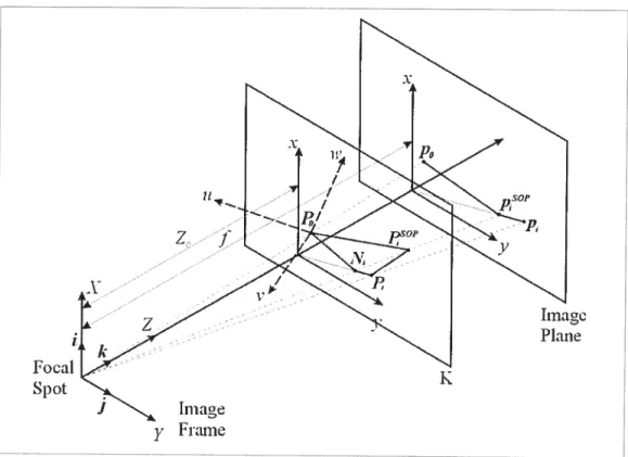
POSIT (Pose from Orthography and Scaling with Ileration) [6, 14] has been developed by DeMenthon and Davis. The method approximates the perspective projection with a scaled orthographic projection (SOP), also known as weak perspective projection, and estimates the pose by solving a linear system. The above process is iterated to achieve more accurate pose by optimized SOP.

The scheme of the POSIT method is depicted in Figure 2.4. The model reference frame is centered at P0 and its coordinate system is (u, y, w). The origin of camera is at

the focal spot and its coordinate system is (X Y, Z), with i,

_j,

and k representing the unit vectors along X, Y, and Z axes, respectively. The object point P1 in the camera reference frame is represented as P = [X, Y, Z1], and its perspective projection and SOP are

represented as p. =[x ]T and =[x’,y]T, respectively. Plane K is through Po and

parallel to the image plane.

The goal of the POSIT rnethod is to compute the rotation matrix and translation vector of the object. The rotation R is the matrix whose rows are the coordinates of the unit vector i,j, k ofthe camera reference frame expressed in the object coordinate system

(it, y,w) and is written as:

ju 1, W

R ₌

_J

_J

_i

k k k

where i, i.,, i are the coordinates of j in the coordinate system (u, y, w) of the object, and

similarÏy withj11,j,j and k, k1, Iç.

b compute the rotation, we only need to compute j and

_j

in the model reference ftame. The vector k is then obtained by i x

_j.

The translation T equals to 0F0, and therefore the coordinates of the translation vector are Xo, Yo, Zo. The point po is the projection of point P0 on the image plane; and the translation T is atigned with vector 0p and is equal to --0rn0. Therefore to compute the object translation, we only need to compute its z-coordinate Zo. Thus the object pose if fuÏly defined once we find I,

_j,

and

T

‘ —

fjx, jz,

LX,,YI

_

z0

‘

z0

where [x, y]T is the image ofP with SOP.

The ratio s = is the scaling factor ofthe SOP. The _{point I} {X0,Y0,Z0]T _bas

u,,— z focal Sj)Ot Plane

j

[mage

L____

y frame

figure 2.4 _{Scheme of the POSIT method. The image p is the perspective projection of object}

pointF _{and image p°” is the scaled orthographic project (SOP) of the object pointF. K is the}

plane throughFand parallel to the image plane.

The POSIT method is based on using SOP to approximate the perspective projection. Here, we choose Zo as the depth of SOP and therefore SOP ofP1= [Xj, Y1, Z]T

is expressed as:

(2.26)

21

From figure 2.4, we have

0 (2.27) jj7 _{.2_j=y.(1+E.)—y0}

z0

where E. is defined as (2.2$) andkis k=ixj. (2.29)

The proof of equation (2.26) is given in [4]. Equation (2.27) can be rewritten as

jj .J=x(1+E)—x (2.30) pp .J=y(1+E)—y where I =

Li

(2.31) J=

j_i.

z0

Given an estimate of E., equation (2.30) provides a linear system of equations in which

the only unknowns are the coordinates of I and J. The linear systems of equation (2.3 1) can be solved by using Linear Least Square method [7].

The P0511 algorithm starts with an estimate of E1, say E. = 0, and solves equation

(2.30). Then a more accurate E. is obtained by flrstly computing i andj through equation

(2.3 1), then k through equation (2.29), flnally E. through equation (2.2$). The above

process adjusts E. until the change of E1 between the current and previous iterations is

sufficiently small.

In order to meet the atgorithm requirement that the object point P0 must be located

at the origin of the model reference frame, the translation, T’, applied to the initial model

noted as:

I” =[I.”j” +T’, _(2.32)

where _{[1” ]“ represents object points in the initial model reference frame as the input of} the algorithrn. Inversely, in order to obtain the transformation, T”, in the initial model reference frame, we compute:

T” =T+T’R. _(2.33)

The following is the summary of the algorithm. Preprocess according to equation (2.32).

1) Translate the object with 1 so that the Po is located at the origin of the

transformed model reference frame through equation (2.32).

2) Let E, =0, (1 =

3) Compute x.(1+ E/”) —x0 and y(l ÷E)r?l

)

—y0; solve for vectors land Jusing

the Linear Least Square method; and compute j= and

_j

=

SI S2

f

1

4) Compute new E.: using k = txj; Z0 _=—; E1 = —P,P.k.

s Z0

5) If

,

— E/’ Threshold

,

retum the result; else go to step 2.

Postprocess according to equation (2.33). Then retum T,, T2, T3,

_Ø,

and

_Ø.

2.4 Comparison of the Three Methods

Six groups of test data were used; the last three groups are generated randomÏy by a Mathematica program while the first three groups are chosen manuaÏly, and used to test the pose methods presented above. In order to evaluate the noise robustness of the methods, further tests were carried out by adding random noise with maximum amplitude of ±5% to the measured images in the above test data. The test data without noise effect and the resuits are listed in Table 2.1 through Table 2.7, whule the test data by adding noise and the resuits are listed in Table 2.8 through Table 2.14.

following are the main observations that can be made regarding the comparison of these three pose estimation methods from the data in Table 2.1 through Table 2.7.

Li

- The PO$IT method is the most efficient and the most accurate method.

- The POSIT method does not need an initial estimate of rotation and translation, while

both SPT and Newton’s methods need initial estimates.

- The Newton’s method is only suitable for a small range of rotation angles, typically

smaller than 300 _{around the Z-axis, even when a proper initial estimate of rotation}

angles are given. The SPT method is better than the Newton’s method, but is also limited to suitable rotation angles range due to the possibility of solutions faïling into local minima. The drawbacks and a solving strategy are discussed in [11]. The POSIT, _{which does flot need the initial estimates of R and T can be used with any} rotation angles.

In conclusion, according to our simulation, the POSIT method demonstrates fairly good performances in terms of accuracy, efficiency, and is suitable for the whole rotation range.

Compare the test results between the data in Table 2.1 through Table 2.7 and the data in Table 2.1 through Table 2.7, we can see that when adding random noise to the rneasured images, the accuracy of the POSIT is affected significantly. For most of cases, for example: the data in Table 2.8, Table 2.9, Table 2.11, Table 2.12, and Table 2.13, the enors by the POSIT are even worse than the enors by SPT method.

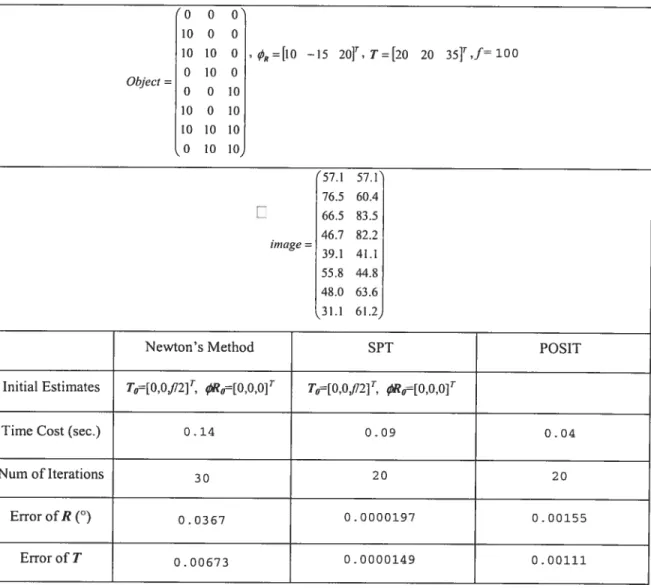
Table 2.1 Within a smalt rotation around the Z-axis, Newton’s method, SPT method, and POSIT obtain proper solutions. SPI demonstrates a good performance in terms of accuracy, while POSIT demonstrates a good performance in terms of efficiency.

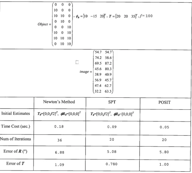
o o 0’ 10 0 0 10 10 0 _ØR=[iO —15 20]T, _{r=[2o 20} 351T,.f 100 0 10 0 Objeci= 0 0 10 10 0 10 10 10 10 0 10 10, 57.1 57.1’ 76.5 60.4 t 66.5 83.5 46.7 82.2 image= ‘ 39.1 41.1 55.8 44.8 48.0 63.6 31.1 61.2

Newton’s Method SPI POS1T

Initial Estirnates T0=[0,0112]T, 0R0=[000IT T0[O,Oj72]T, 0j000jT

TirneCost(sec.) 0.14 0.09 0.04

Numofiterations ₃₀ 20 20

ErrorofR(°) 0.0367 0.0000197 0.00155

25

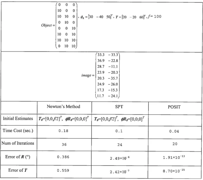
Table 2.2 _{Within a small rotation around the Z-axis, Newton’s method, SPI method and POSIT} obtain proper solutions. POSIT demonstrates good performances in terrns of accuracy and efficiency. ‘0 0 0 10 0 0 10 10 0 ØR30 —40 5o, T=î20 —20 60],f 100 0 10 0 Object= 0 0 10 10 0 10 10 10 10 0 10 10, 33.3 —33.3 36.9 —22.8 28.7 —11.1 23.9 —20.3 image= 20.3 —35.7 24.9 —26.0 17.3 —15.3 11.7 —24.1

Newton’s Method SPT POSIT

Initial Estirnates T0=[O,0f72]T, _{ØR[O,O,0]’} T0{O,Ofi2]T, 0R0[O,O,O]T

lime Cost (sec.) 0.18 0.1 0.04

Num oflterations _{36 24} 20

ErrorofR(°) 0.386 _2.49x10 1.91X10’3

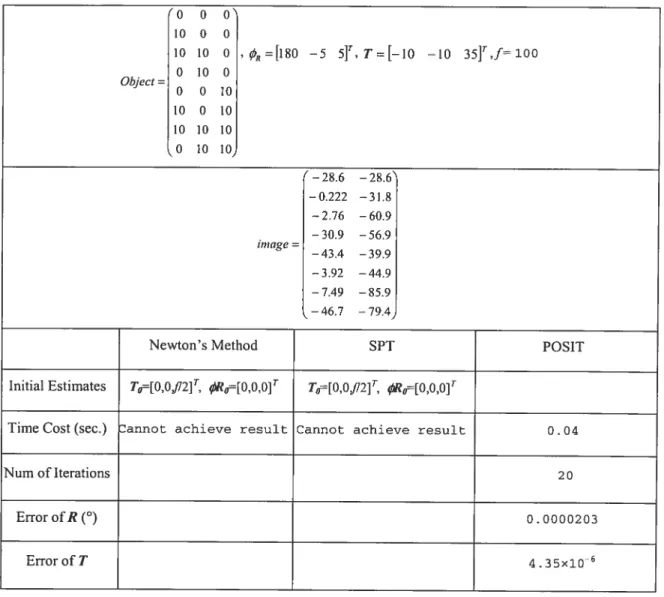
Table 2.3 _{With this test data, both Newton’s method and SPT method cannot obtain a proper} solution. 0 0 0 10 0 0 10 10 0 ,ØR=[180 —5 s]T,r=[—io —10

35Ï’f’100

0 10 0 Object= 0 0 10 10 0 10 10 10 10 O 10 10 ‘ —28.6 —28.6 —0.222 —3].8 —2.76 —60.9 • —30.9 —56.9 image= —43.4 —39.9 —3.92 —44.9 —7.49 —85.9 —46.7 —79.4

Newton’s Method SPI POSIT

Initial Estimates T11=[0,0J12JT, 0R0=[0,0,0]T T0=[0,0,fl2JT, 0R0=[000]T

TimeCost(sec.) annot achieve resuiL Cannot achieve resuit 0.04

Num oflterations 20

ErrorofR(°) 0.0000203

27

Table 2.4 _{The same test data as in Table 6.1 (cl), but a proper set of initial estimates of rotation} angles are given, SPT obtains a proper solution, while Newton’s method still fails to find the solution. 0 0’ 10 0 0 10 10 0 , ØR=[18O 5 5]T, T=[—l0 —10 35]Tf=100 0 10 0 Object O O ]0 10 0 10 10 10 10 0 10 10 —28.6 —28.6 —0.222 —31.8 —2.76 —60.9 • —30.9 —56.9 image= —43.4 —39.9 —3.92 —44.9 —7.48 —85.9 —46.7 —79.5

Newton’s Method SPT POSIT

Initial Estimates T0=[0,O,fl2]’,ØR0=[150,20,20]’ T0=[O,Oj72]T,?o=[_{150,20,20]’}

TimeCost(sec.) Cannot achieve resuit Cannot achieve resuit 0.04

Num oflterations ₂₀

ErrorofR(°) 0.0000203

Table 2.5 _{With this test data, Newton’s mcthod fails to find the solution. POSIT method} demonstrates better performance in terms of efficiency and accuracy.

‘0 0 0 10 0 0

10 io o , øR=[60 5 6O1,

r[—io

—w 7o],f=100

0 10 0 Object 0 0 10 10 0 10 10 10 10 0 10 10 f_]43 —14.3 —6.45 —7.78 —16.7 —3.54 • —25.1 —9.25 image= —14.4 —24.8 —7.12 —17.7 —16.7 —13.2 —24.7 —19.6

Newton’s Method SPT POSIT Initial Estimates T0=[0,0j72]T, j0[000]T _{T0=[0,0.112]T,}

ØR0=[0,0,0]T

TimeCost(sec.) CannDt achieve recuit 0.1 0.04

Num oflterations ₂₀ 20

ErrorofR(°) _6.55x105 3.02x10’4

29

Table 2.6 With this test data, Newton’s method failed to find the solution. The POSIT method demonstrates better performance in terms of efficiency and accuracy.

—5 —3 10 — [207 —49 22

J,

T=[—30 17 40f ,f=100 Object= —10 9 —3 —5 —7 —4 —10 4 1, —103 59.3 —68.7 24.4 image= —74.8 15.9 —59.5 47.5 —81.0 29.2

Newton’s Method SPT POSIT

Initial Estirnates T0=[0,0jÏ2]’, ØR0=[O,O,O]T T0=[O,O,fi2]T, Ø0[o00]T

TimeCost(sec.) Cannot achieve resuit 0.07 0.04

Num of Iterations ₂₀ 20

EfforofR(°) _2.17 4.09x106

Table 2.7 With the test data, Newton’s rnethod failed to find the solution. The POSIT method demonstrates better performance in terms of efficiency and accuracy.

4 —9 7 10 5 —9 ‘ = [29$ —65 24]T, T=9 —4 4l]T,f=iOO Object= —2 5 —2 7 —8 1 11.1 2.66 58.2 6.87 image 25.7 —17.0 24.7 4.06

Newton’s Method SPT POSIT

Initial Estirnates T0=[O,OJÎ2JT, j0[000JT _{T0{0,O,fl2]T. 0R0[000lr}

TirneCost(sec.) Cannot achieve recuit 0.07 0.04

Num oflterations ₂₀ 20

ErrorofR(°) 0.153 3.Q5x1Q8

31

Table 2.8 _{By adding random noise with maximum amplitude of ±5% to the measurcd images in} the test data in Table 2.1, it is shown in this case that the errors of the resuit by the POSIT become larger than the errors of the result by the $PT. Newton’s method still lias the largest errors in its result.

‘0 0 0’ 10 0 0 10 10 0 _ØR=î10 —15 20]T, T=[20 20 35]Tf=100 0 10 0 Object= 0 0 10 10 0 10 10 10 10 0 10 10 •54.7 54.7 74.2 58.6 D 69.5 87.2 • 45.6 $0.3 image= 38.9 40.9 56.9 45.7 47.4 62.7 32.2 63.3

Newton’s Method SPT POS1T

Initial Estirnates T0=[0,0,fl2]T, 0R0=[000]T _{T0=[0,0J12f, ?0=[O,O,O]T}

Tirne Cost (sec.) 0. 1$ 0.09 0.05

Numoflterations ₃₆ 20 20

ErrorofR(°) _6.88 5.08 5.80

Table 2.9 _{By adding random noise with maximum amplitude of}±5% to the measured images in the test data in Table 2.2, it is shown in this case that the errors ofthe resuits by the three methods

have no significant differences.

‘0 0 0’ 10 0 0 10 10 0 , ÔR30 —40 50]T T=[20 —20 601T,f 100 O ]0 O Object= 0 0 10 10 0 10 10 10 10 0 10 10, ‘33.4 —33.4’ 36.1 —22.3 28.9 —11.2 • 24.0 —20.3 image= 19.9 —35.1 24.2 —25.2 17.0 —15.1 11.8 —24.2,

Newton’s Method SPT POSIT

initial Estirnates T,)={O,0J72]T,

ØR0=[O,O,O]’ T[O,Of12]‘, 0R0{O,O,O]T

Tirne Cost (sec.) 0.17 0.09 0.04

Num ofiterations _{36 20 20}

ErrorofR(°) 3.66 _2.91 3.81

33

Table 2.10 By adding random noise with maximum amplitude of±5% to the measured images

in the test data in Table 2.3, it is shown in this case that the errors of the resuit by the POSIT

become significant large.

‘0 0 0’ 10 0 O 10 10 O R=[180 —5

51’

r=[—io

—10 351T,f=100 0 10 0 Object= 0 0 10 10 0 10 10 10 10 0 10 10, —27.1 —27.1 —0.217 —31.1 —2.88 —63.6 —29.7 —54.6 image —43.8 —40.2 —3.97 —45.5 —7.65 —87.8 —46.0 —78.3

Newton’s Method SPT POSIT

Initial Estimates T0=[0,0,112JT, ØR=[ooOjT _{T0=[0,0.f72j” 0R0=[000]T}

TirneCost(sec.) annot achieve resuit Cannot achieve resuit 0.04

Num oflterations 20

ErrorofR(°) 1.14

Table 2.11 _{By adding random noise with maximum amplitude of}+5% to the measured images in the test data in Table 2.4, it is shown in this case that the errors of the result by the POSIT

become much larger than the errors shown in Table 2.4.

‘0 0 0 10 0 0 10 10 0 ‘ 01? =[180 —5 5]’, T=[—10 —10 35j’,f 100 0 10 0 Object= 0 0 10 10 0 10 10 10 10 10 10 —27.3 —27.3 —0.217 —31.0 —2.84 —62.8 • —31.8 —58.4 iiiiage= —44.1 —40.6 —4.08 —46.8 —7.51 —86.1 ‘—45.8 —77.8,

Newton’s Method SPT POSIT

Initial Estirnates T0=[0,0,J12]TØJ?0[_{150,20,20]’} T0=[0,0j12]T_{ØR0=[150,20,20]}T

TirneCost(sec.) Cannol achieve result Cannot achieve resuit 0.04

Num oflterations 20

ErrorofR(°) 3.19

35

Table 2.12 By adding random noise with maximum amplitude of±5% to the measured images

in the test data in Table 2.5, _{it is shown in this case that the errors of the result by the POSIT}

become larger than the errors of the restiit by the SPT.

O O 10 O O 10 10 0 , ØR=[60 —5 60]’, Tz[_J0 —10 70]T,f 100 0 10 0 Object= 0 0 10 10 0 10 10 10 10 0 10 10 ‘—14.2 —14.2 —6.70 —8.08 —17.0 —3.61 • —26.3 —9.67 image= —14.0 —24.1 —7.13 —17.7 —17.2 —13.6 —25.4 —20.2

Newton’s Method SPI POSIT

Initial Estimates T0=[0,0,/12]T, 0[000jT

T0=[0,0j12j, ØR=[0.0,01’

TirneCost(sec.) Cannot achieve recuit 0.1 0.04

Numoflterations _{20 20}

ErrorofR(°) _{0.648 1.58}

Table 2.13 _{By adding random noise with maximum amplitude of +5% to the measured images}

in the test data in Table 2.6, it is shown in this case that the errors of the resuit by the PO$IT

become as large as the errors ofthe result by the SPT..

—5 —3 10 ‘0k [207 —49 22 T=[—30 17 40]T ‘1=100 Object={—1Û 9 —3 —5 —7 —4 —10 4 1 —102 58.9 —67.3 23.9 image= —75.8 16.1 —60.8 48.5 —77.9 28.1

Newton’s Method SPI POSIT

Initial Estirnates T0=[0,0,JÏ2]T, _{ØR0={0,0,0]’} T0=[0,0j721T, 0{0001T

TirneCost(sec.) Cannot acheva result 0.1 0.04

Num oflterations _{20 20}

ErrorofR(°) _5.38 2.76

37

Table 2.14 By adding random noise with maximum amplitude of±5% to the measured images

in the test data in Table 2.7, it is shown in this case that the errors of the resuit by the POSIT become larger than the errors ofthe result by the SPT.

4 —9 7 10 5 9 = [298 —65 24]T T=[9 4J]rf= 100 Object= —2 5 —2 7 —$ 1 11.5 2.75 . 59.7 7.05 image= 24.5 —16.2 23.7 3.90

Newton’s Method SPT POSIT

Initial Estirnates T,[0,0,fl2jT øRj[ooo]T T0=[0,0,f121T, 0[lJoiJ]T

TimeCost(sec.) ‘annot achieve result 0.07 0.04

Num oflterations ₂₀ 20

ErrorofR(°) _1.44 13.1

2.5 Summary

In the reconstruction of vessels from WUS images, biplane angiography or single projection angiography is needed. Biplane angiography bas the drawbacks of the expensive equipment, complex operation, and requirement of calibration. Because single projection _{angiography overcomes most of the drawbacks existing in bipÏane} angiography, it has drawn increasing attention from researchers.

Single projection angiography employs the method of pose estimation by single projection. Among many publications on pose estimation by single projection, we have studied three methods. They are Newton’s method, SPI, and POSIT. The simulation resuits have shown that the POSIT method is the best method in terms of accuracy, efficiency, and stability among the methods we have studied.

Although single projection angiography overcomes the drawbacks existing in biplane angiography, on the other hand, it requires a prior knowledge of the 3-D configuration of vessels. In the next chapter, we wiÏl investigate the possibility and propose a method of using an image sequence taken by single projection angiography to reconstruct a trajectory of catheter in IVUS intervention without a prior knowledge of configuration of vessels.

39

Chapter 3

A Method of Pose Estimation by an Image

$equence from Single Projection

3.1 Introduction

As presented in Chapter 2, in the reconstruction of catheter trajectory in 3-D IVUS artery _{intervention, either biplane angiography or single projection angiography is} employed to provide the information of location and orientation for each frarne ofWUS images. Single projection angiography has advantages of low equipment cost and is easier to operate over biplane angiography and therefore has drawn a lot of attention from researchers. Kowever, for single projection angiography, there exists a limitation that a 3-D configuration of artery is required. That is due to the fact that the method of pose estimation by single projection, which is used in single projection angiography, requires prior knowledge of the 3-D configuration of the object. The 3-D configuration of artery can be obtained by computed tomography (CT) or magnetic resonance (MR). This consequently increases clinical cost.

In this chapter, we propose a nove! method of pose estimation with image sequence taken from a single view. Compare with the methods discussed in Chapter 2, the proposed method only needs the measurement of pullback length of the catheter, instead of the requirement of the knowledge of the 3-D configuration of the object, instead. In a typical IVUS intervention, an angiographic sequence from single projection can be taken to localize the IVUS transducer during its pullback. Based on this fact, we propose a new method of pose estimation with an image sequence taken from a single view with no need of prior knowledge of the object 3-D configuration, targeting for an implementation in angiography. The proposed method avoids the additional CT or MR

imaging used in single projection angiography, and thus reduces the clinic cost and simplifies the IVUS investigation.

The proposed method is simulated in Mathematica by using a given spiral curve to represent the configuration of an artery. Several cases are implemented with various locations, orientations, and sizes ofthe given curve.

The chapter is organized as follows. In Section 2, we describe the configuration of an angiography system during an IVUS intervention. In Section 3, we present in detail our new method of pose estimation with an image sequence from single projection. In Section 4, we present the simulation of the proposed method in Mathematica. In Section 5, we give a summary of this chapter.

3.2 Angiography in IVUS intervention

In a typical 3-D IVUS _{intervention, angiography is used to determine the location} and orientation ofIVUS images. In this section, we describe the configuration ofa typical angiography system geometrically. A set of typical measurements for the configuration is given, which will be used in the simulation ofthe proposed rnethod.

Figure 3. 1 shows the configuration of a coronaiy angiography system for 3-D IV US. The focal length,

_f

_{is the distance from a focal spot (i.e., X-ray source) to the} image plane. The patient is located between the focal spot and the image plane. We use ci to indicate the distance from the focal spot to the centre ofthc patient’s heart. Notice that cl cannot be measured accurately. In a 3-D IVUS intervention, a miniaturized ultrasonic transducer at the end of a catheter is inserted in the artery lumen, and then withdrawn gradually. An image sequence is taken during the pultback of the catheter. The pullback length of a catheter between grabbing images i and image i+] is indicated as AI,. as shown in f igure 3.2. In the following discussion, we assume that /l000m,n and c/=500mnz. The size of the heart is within a sphere of radius r=lOOmm. These assumptions for measurements are close to the real clinical situation.

41

3.3 A Method of Pose Eslimation with an Image Sequence from Single Projection

In this section, we propose a method _{of pose estimation with an image sequence}

from single projection. The rnethod is intended to be irnplernented for the reconstruction

ofthe trajectory ofa catheter from an image sequence taken by single angiography. In the

foïlowing discussion, the trajectoty ofa catheter is viewed as a 3-D curve.

This section is otganized as fotlows. In subsection I, we geometrically analyze the problem of pose estimation by an image sequence from single projection. In subsection 2, we discuss how to find multi-solutions for the trajectory curve. A strategy for eliminating invalid solutions using physical characteristics of the catheter path is presented in subsection 3. In subsection 4, we discuss the strategy that we use to reduce the accumulated error. in subsection 5, we discuss how to determine the location ofthe start point of the trajectory curve. _{In the last subsection, we summarize the proposed}

rnethod.

3.3.1 A Geornetrical Analysis of the Problem of Pose Estimation by an Image Sequence

from Single Projection

We define the coordinate system for an angiography camera system as (X }Ç Z)

with its origin tocated at the focal spot and image plane at Z=J and define the coordinate

system for an image as (x, y), which Lies in the image plane and is parallel to the X and Y

axes. The coordinate systems (X Y, Z) and (x, y) _{are ilÏustrated in igre 3.1. As shown in}

Figure 3.2, P1(X, }, Z) andp1(x1, V) respectively represent the 3-D location ofa catheter

tip and its corresponding projection on the image plane when the i-th coronary angiography image is captured. Since the size of the heart, within a sphere of radius

r_{lOOmm, is significantÏy smaller than the focal Iength, J1 000mm, we assume that}

catheter tip images are caught under a weak perspective projection. furthermore, we assume that the length of the curve, AI1, is srnall enough so that each segment of the trajectory curve can be viewed as a straight une with its length approxirnately equal to

AI1. Based on the above assumptions, the relation between a segment of the trajectory of

the cathetertip, F1P1±1, and its weak perspective image, p,pj±j, as shown in Figure 3.2, can be represented as the following equations:

X1 — X. = (x,1 — x).s (3.1 a) — = —j) s (3. lb) Z11 Z = ±AÏ —(x÷1 —x)2 $2 — — , (3.1 e)

where s = a scale factor for weak perspective projection. and AÏ1 is the pullhack

length of the catheter in the interval between capturing the i-th image and capturing the i+Ï-th image.

Based on the assumption of weak perspective projection, the X and Y-coordinates

of the point on the trajectoly coiiesponding to a point in the image can be estirnated by

fol lowing equations:

X. =sx.

(3.2)

Iç =syi.

Furthermore, we assume that the Z-coordinate of the start point of the trajectory curve, noted as Z1, is known, and the length ofpullback ofcatheter, AÏ1, is known, then Z1 (i>O)

can be computed by using equation (3. Ic). Later in this chapter, we wiLl present a strategy

43

]flia’eptJnY —

X :rh,’t,’ïri;’

J 100(1 - 2r,jjec ton’0’cot/wrr1,

--s

/7’

/ EoccIÏ0t _V

figure 3.2 A segment of trajectory ofa cathetertipand its projection on the image plane

J

Ft)a1spot

Figure 3.3 11 is the plane that passes through the point F+ and is parallel to the X and Y-axis,

_Ø

is the angle between the une ofFP1÷1 and the plane H.