Automatic Multilevel Temporal Video Structuring

HAL Id: hal-00735694

https://hal.archives-ouvertes.fr/hal-00735694

Submitted on 26 Sep 2012

HAL is a multi-disciplinary open access

archive for the deposit and dissemination of

sci-entific research documents, whether they are

pub-lished or not. The documents may come from

teaching and research institutions in France or

abroad, or from public or private research centers.

L’archive ouverte pluridisciplinaire HAL, est

destinée au dépôt et à la diffusion de documents

scientifiques de niveau recherche, publiés ou non,

émanant des établissements d’enseignement et de

recherche français ou étrangers, des laboratoires

publics ou privés.

Automatic Multilevel Temporal Video Structuring

Ruxandra Tapu, Titus Zaharia

To cite this version:

Ruxandra Tapu, Titus Zaharia. Automatic Multilevel Temporal Video Structuring. 2011 IEEE Fifth

International Conference on Semantic Computing, Sep 2011, Palo Alto, California, United States.

pp.387-394. �hal-00735694�

Automatic Multilevel Temporal Video Structuring

Ruxandra Tapu and Titus Zaharia

Institut Télécom / Télécom SudParis, ARTEMIS Department, UMR CNRS 8145 MAP5

Evry, France

email: {ruxandra.tapu, titus.zaharia}@it-sudparis.eu Abstract—In this paper we propose a novel and complete video

scene segmentation framework, developed on different structural levels of analysis. Firstly, a shot boundary detection algorithm is introduced that extends the graph partition method with a nonlinear scale space filtering technique which increase the detection efficiency with gains of 7,4% to 9,8% in terms of both precision and recall rates. Secondly, static storyboards are formed based on a leap keyframe extraction method that selects a variable number of keyframes, adapted to the visual content variation, for each detected shot. Finally using the extracted keyframes, spatio-temporal coherent shots are clustered into the same scene based on temporal constraints and with the help of a new concept of neutralized shots. Video scenes are obtained with average precision and recall rates of 86%.

Keywords-shot boundary detection; two-pass approach; temporal constraints; shot merging

I. INTRODUCTION

Recent trends in telecommunications collaborated with the expansion of image and video processing and acquisition devices has lead to the rapid growth of the amount of data stored and transmitted over the Internet. Existing commercial and industrial video searching engines are currently based solely on textual annotations, which consist of attaching some keywords to each individual item in the database.

When considering video indexing and retrieval applications, we first have to address the issue of structuring the huge and rich amount of heterogeneous information related to video content. Keyframes, shots, and scenes are the traditional elements that need to be determined and described.

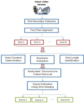
The analysis framework proposed in this paper is illustrated in Fig. 1. Our contributions concern the optimized shot boundary detector, a novel keyframe selection algorithm and a shot grouping mechanism into scenes based on temporal constraints.

The rest of this paper is organized as follows. After a brief recall of some basic theoretical aspects regarding the graph partition model exploited, Section II introduces the proposed shot detection algorithm. In Section III, we describe the keyframe selection procedure. Section IV introduces a novel scene extraction algorithm based on hierarchical clustering and temporal constraints. In Section V we present and analyze the experimental results obtained. Finally, Section VI concludes the paper and opens perspectives of future work.

Figure 1. Scene change detection algorithm. II. SHOT BOUNDARY DETECTION SYSTEM

The development of shot-boundary detection algorithms was explosive in the last decade, as witness the rich scientific literature dedicated to this topic. The simplest way to determine a camera brake is based on the absolute difference of pixels color intensities, between two adjacent frames. Obviously, such methods are highly sensitive even for reduced local object and camera motion, since they capture all details in a frame [1], [2]. A natural alternative to pixel-based approaches are histogram-based representation, due to the spatial invariance properties [3], [4]. Methods based on edges/contours have inferior performances compared to algorithms implementing color histogram, although the computational burden is greater [5]. However, such edge features find their applications in removing false alarms caused by abrupt illumination [3]. Algorithms using motion features [6] create an alternative to pixel and histograms based methods due to their robustness to camera and object displacement. The techniques developed in compressed domain assure optimal processing time [7], but provide inferior precision and recall rates than histogram based approaches.

In this section, we propose an improved shot boundary detection algorithm, based on the graph partition (GP) model

introduced in [3] and considered as state of the art for both abrupt (cuts) and gradual transition (fades, wipes…) detection.

A. Graph Partition Model

Let us first recall the considered model introduced in [8]. The video sequence is represented as an undirected weighted graph. We denote by G an ordered pair of sets (V, E) where V represents the set of vertices, V = {v1,v2,…,vn}, and E

⊂

V × V

denote a set of pair-wise relationships, called edges. An edge

ei,j = {vi, vj} is said to join the vertices vi and vj, that are

considered neighbors (or adjacent). In the shot boundary context, each frame of the video is represented as a vertex in the graph structure, connected with each others, by edges. To each edge eij, a weight wij is associated to, which expresses the

similarity between nodes vi and vj. In our case, we considered

the chi-square distance between color histograms in the HSV color space defined as follows:

∑ × − + − = k j i e j k H i k H j k H i k H j i w | | 2 ) ( , . (1)

where H i _{denotes the HSV color histogram associate to}

frame i. The exponential term in (1) is used in order to take into account the temporal distance between frames: if two frames are located at an important temporal distance it is highly improbable to belong to the same shot.

The video is segmented using a sliding window that selects a constant number of N frames, centered on the current frame

n. A sub-graph Gn is thus computed for each frame n, together

with the similarity matrix Sn which stores all the distances

(weights) between the N nodes (frames) of the graph. Let

Vn = {vn1, vn2,..., vnN} denote the vertices of graph Gn at frame n.

For each integer k € {1,...,N-1}, a partition of the graph Gn into

two sets

(

{

}

{

N

}

)

n k n k n k n n k n v v B v v A = 1,…, , = +1,…, is defined. To each partition, the following objective function is associated with:

) ( ) , ( ) ( ) , ( ) , ( k n k n k n k n k n k n k n k n B assoc B A cut A assoc B A cut B A Mcut = + . (2)

where cut and assoc respectively denote the measures of cut (i.e. dissimilarity between the two elements of the partition) and association (i.e. homogeneity of each element of the partition) and are defined as described in (3) and (4):

∑

∈ = k n A j i j i k n w A assoc , , ) ( ;

∑

∈ = k n B j i j i k n w B assoc , , ) ( . (3)

∑

∈ ∈ = k n k n,j B A i i,j k n k n,B ) w cut(A . (4)

The objective is to determine the optimal value of k which maximizes the objective function in (2). In this way, the cut between the elements of the partition is maximized while the corresponding associations are simultaneously minimized.

Finally, the maximal value of the Mcut measure is associated to frame n. A local dissimilarity vector v is thus constructed. For each frame n, v(n) is defined as:

{ }

{

(

)

}

k n k n 1 -, 1, k max A ,B ) (n Mcut v N … ∈ = . (5)

A straightforward manner to detect shot transitions is to determine peaks in the dissimilarity vector v that are greater than a pre-defined threshold value Tshot. However, in practice,

determining an optimal value for the threshold parameter Tshot

is a difficult challenge because of large object motion or abrupt and local changes of the lightening conditions, leading to both false alarms and missed detections. For these reasons, in contrast with [3] and [8], we propose to perform the analysis within the derivatives scale space of the local minimum vector v, as described in the next section.

B. Scale Space Filtering

More precisely, if we consider v’(n) the discrete derivative of vector v(n), defined using the first order finite difference (v’(n) = v(n) – v(n–1)), we construct a set of cumulative sums

{ }

N k k n

v'( ) ₌₁, over the difference signal v(n) up to order N, by

setting:

∑

= − = k p k n v n p v 0 ' ' _{( ) ( ). (6)}

The signals v’k(n) can be interpreted as low-pass filtered

versions of the derivative signal v’(n), with increasingly larger kernels, and constitute our scale space analysis. After summing all the above equations v’k(n) can be simply expressed as:

) ( ) ( ) ( ' _{n v n v n k} vk = − − . (7)

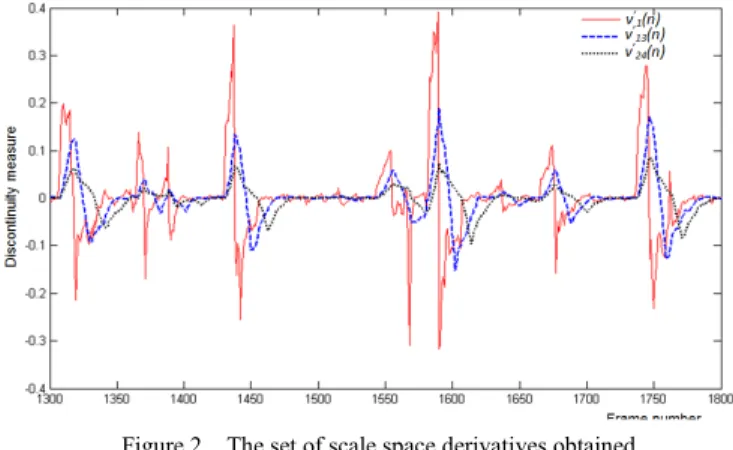
Fig. 2 illustrates the set of derivatives signals obtained when using our algorithm. We can observe that smoother and smoother signals are produced, which can be helpful to eliminate variations related to camera/large object motions. The peaks which are persistent through several scales correspond to

large variations and can be exploited to detect transitions. Figure 2. The set of scale space derivatives obtained.

In order to detect such peaks, we first apply a non-linear filtering operation to the multi-scale representation. More precisely, we construct the following filtered signal:

{

( )

}

max

{

( ) ( ) ( )

}

max ) (n v' hk v n v n k h k d k k k ⋅ = − − ⋅ = (8)

where the weights h(k) are defined as:

⎪ ⎪ ⎩ ⎪⎪ ⎨ ⎧ ⎥⎦ ⎤ ⎢⎣ ⎡ + ∈ ⎥⎦ ⎤ ⎢⎣ ⎡ − ∈ = − − − N N k e N k e k h k N k , 2 1 , 2 1 , 0 , ) ( 1 . (9)

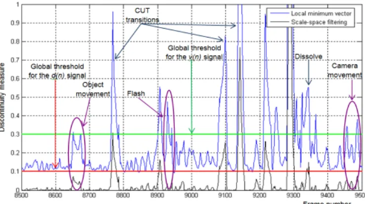
The shot detection process is applied on the d(n) signal thus obtained. The weighting mechanism adopted privileges derivative signals located at the extremities of the scale space analysis (Fig. 3). In this way, solely peaks that are persistent through all the considered scales are retained.

C. Two Pass Approach

We focused next on reducing the computational complexity of the proposed algorithm by introducing a two-step analysis technique. In a first stage, the algorithm detects video segments that can be reliable considered as belonging to the same shot. Here, a simple (and fast) chi-square comparison of HSV color histograms associated to each pair of consecutive frames is performed, instead of applying the graph partition model. In the same time, abrupt transitions presenting large discontinuity values are detected.

In the second stage, we consider the scale space filtering method described above, but applied uniquely to the remaining uncertain video segments. This second step makes it possible to distinguish between gradual transitions and fluctuations related to large camera/object motion.

For each detected shot, we aim to select a set of keyframes that might represent in a pertinent manner the associated content.

III. KEYFRAME EXTRACTION

One of the first attempts to automate the extraction process was to choose as a key frame the first, the middle or the last picture appearing after each detected shot boundary [9] or even a random image within a shot. However, while being sufficient for stationary shots, one frame does not provide an acceptable representation of the visual content in the case of dynamic sequences that exhibit large camera motion. Therefore, it is necessary to implement more complex methods [10] which aim at removing all redundant information. In [11] the extraction process relay on the color and motion features variation within the considered shot. Different approaches use clustering techniques to find optimal keyframes [12]. Even so, clustering techniques have weak points related to the threshold parameters which control the cluster density and the computational cost. A mosaic-based approach can generate, a panoramic image of all informational content existed in a video stream [13]. However, mosaics can blur certain foreground objects and thus, the

resulted image cannot be exploited for arbitrary shape object recognition tasks.

In our case, we have developed a key-frame representation system that extracts a variable number of images from each detected shot, depending on the visual content variation. The first keyframe extracted is selected by definition, N (i.e., the window size used for the shot boundary detection) frames away after a detected transition, in order to verify that the selected image does not belong to a gradual effect. Next, we introduced a leap-extraction method that consider for analysis only the images located at integer multipliers of window size and not the entire video flow as [11], [14]. The current frames are compared with the existing shot keyframes set already extracted. If the visual dissimilarity (chi-square distance of HSV color histograms) between the analyzed frames is significant (above a pre-establish threshold), the current image is added to the keyframe set (Fig. 4).

By computing the graph partition within a sliding window, our method ensures that all the relevant information will be taken into account. Let us also note that the number of detected keyframes set per shot is not fixed a priori, but automatically adapted to the content of each shot.

Figure 3. False alarms due to flash lights, large object/camera motion are avoided when using the scale-space filtering approach.

In this stage we introduced an additional preprocessing step that eliminates all the monochrome and redundant images [15] from the selected set of keyframes assuring that the story board captures all informational content of the original movie without any irrelevant images, which directly influences the representative power of the summary [16].

IV. SCENE SEGMENTATION

In the recent years various methods to partition video into scenes have been introduced. In [14], authors transform the detection problem into a graph partition task. In [17] the detection is based on the concept of logical story units and inter-shot dissimilarity measure. Different approaches [18] proposed combine audio features and low level visual descriptors. In [19] color and motion information are integrated in the decision process. A mosaic approach is introduced in [13] that use information specific to some camera setting or physical location to determine boundaries. More recent techniques [18], [19] apply concepts as temporal constraints and visual similarity.

We present further our novel scene detection algorithm based on hierarchical clustering and temporal constraints. Considering the previously extracted keyframes we construct a clustering system by iteratively merging shots falling into a temporal analysis window and satisfying certain grouping criteria. The width of the temporal analysis window, denoted by dist, is set as proportional to the average number of frames per shot: shots of number Total frames of number Total dist=α⋅ , (10)

with α a user-defined parameter. We consider further that a scene is completely described by its constituent shots:

{

}

Nl p n i f l N p p l s S s : l S _{l l pi} lp 1 1 ) 1 , ) ( _{, ,} , = ⎪⎭ ⎪ ⎬ ⎫ ⎪⎩ ⎪ ⎨ ⎧ = → = ⎭ ⎬ ⎫ ⎩ ⎨ ⎧ = , (11)

where Sl denotes the lth video scene, Nl the number of shots

included in scene Sl, sl,p the pth shot in scene Sl, and fl,p,i the ith

keyframe of shot sl,p. containing nl,p keyframes.

Our scene change detection algorithm based on shot clustering consists of the following steps:

Step 1: Initialization – The first shot of a film is

automatically assigned to the first scene S1. Scene counter l is

set to 1.

Step 2: Shot to scene comparison – Consider as current shot

scrt the first shot which is not yet assigned to any of the already

detected scenes. Detect the sub-set Ω of scenes anterior to scrt

and located at a temporal distance inferior to parameter dist. Compute the visual similarity between the current shot and each scene Sk in the sub-set Ω, as described in the following

equation: crt k p k matched k crt k n N n n S s im SceneShotS S ⋅ ⋅ = Ω ∈ ∀ , ) , ( , , (12)

where ncrt is the number of keyframes of the considered shot

and nmatched represents the number of matched keyframes of the

scene Sk. A keyframe from scene Sk is considered to be

matched with a keyframe from shot scrt if the visual similarity

measure between the two keyframes is superior to a threshold

Tgroup. Let us note that a keyframe from the scene Sk can be

matched with multiple frames from the current shot.

Finally, the current shot scrt is identified to be similar to the

scene Sk if: 5 . 0 ) , (Sk scrt ≥ im SceneShotS . (13)

In this case, the current shot scrt will be clustered in the

scene Sk. In the same time, all the shots between the current

shot and the scene Sk will be also attached to scene Sk and

marked as neutralized. Let us note that the scenes to which initially belonged such neutralized shots disappear (in the sense that they are merged to the scene Sk). The list of detected

scenes is then updated.

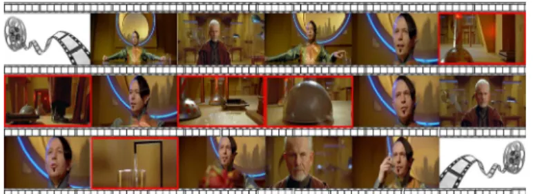
The neutralization process allows us to identify the most representative shots for a current scene (Fig. 5), which are the remaining non-neutralized shots. In this way, the influence of outlier shots which might correspond to some punctual digressions from the main action in the considered scene is minimized.

If the condition described in equation (13) is not satisfied, go to step3.

Step 3: Shot by shot comparison – If the current shot (scrt) is

highly similar (i.e., with a similarity at least two times bigger

than the grouping threshold Tgroup) with a shot of any scene in

the sub-set Ω determined at step 2, then scrt is merged in the

corresponding scene together with all the intermediate shots. If

scrt is found highly similar to multiple other shots, than the

scene which is the most far away from the considered shot is retained.

Both the current shot and all its highly similar matches are unmarked and for the following clustering process will contribute as normal, non-neutralized shots (Fig. 6). This step ensures that shots highly similar with other shots in the previous scene to be grouped into this scene and aims at reducing the number of false alarms.

Step 4: Creation of a new scene – If the current shot scrt

does not satisfy any of the similarity criteria in steps 2 and 3, a new scene, including scrt, is created.

Step 5: Refinement - At the end, scenes including only one

shot are attached to the adjacent scenes depending on the maximum similarity value. In the case of the first scene, this is grouped with the following one by default.

Concerning the keyframe visual similarity involved in the above-described process, we have considered two different approaches, based on (1) chi-square distance between HSV color histograms, and (2) the number of matched interest points determined based on SIFT descriptors with a Kd-tree matching technique [20].

The grouping threshold Tgroup is adaptively established

depending on the input video stream visual content variation as the average chi-square distance / number of interest points between the current keyframe and all anterior keyframes located at a temporal distance smaller then dist.

V. EXPERIMENTAL RESULTS

In order to evaluate our shot boundary detection algorithm, we have considered a sub-set of videos from the “TRECVID 2001 and 2002 campaigns”, which are available on Internet (www.archive.org and www.open-video.org). The videos are mostly documentaries that vary in style and date of production, while including various types of both camera/object motion (Table 1).

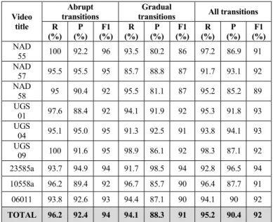
Table 2 presents the precision, recall and F1 rates obtained for the reference graph partition shot boundary detection method proposed by Yuan et al. [3], while Table 3 summarizes the detection performances of our proposed scale-space filtering approach.

The results presented clearly demonstrate the superiority of our approach, for both types of abrupt and gradual transitions. The global gains in recall and precision rates are of 9.8% and 7.4%, respectively. Moreover, when considering the case of gradual transitions, the improvements are even more significant. In this case, the recall and precision rates are respectively of 94,1% and 88,3% (with respect to R = 81.5% and P = 79% for the reference method [3]). This shows that the

scale space filtering approach makes it possible to eliminate the errors caused by camera/object motion.

TABLE I. MOVIE DATABASE FEATURES

Video

title framesNo. transitionNo. transition Abrupt

Gradual transition

File name Fade

in/ out Dissolve Other type NAD 55 26104 185 107 21 57 - NASA Anniversary NAD 57 10006 73 45 6 22 - NASA Anniversary NAD 58 13678 85 40 7 38 - NASA Anniversary UGS 09 38674 213 44 25 144 - Wrestling Uncertainty UGS 04 23918 242 161 71 10 - Hidden Fury UGS 01 32072 180 86 6 88 - Exotic Terrane

23585a 14797 153 80 2 71 - Adelante _Cubanos

10558a 19981 141 79 20 42 1 _Venture Desert

06011 23918 153 81 26 46 - Egg and Us

Total 203148 1425 723 184 518 1 TABLE II. YUAN ET AL.[3] ALGORITHM’S PERFORMANCE

Video title

Abrupt transitions

Gradual

transitions All transitions R (%) P (%) F1 (%) R (%) P (%) F1 (%) R (%) P (%) F1 (%) NAD 55 96.2 82.4 88 87.2 73.9 80 92.4 78.8 85 NAD 57 86.6 86.6 86 78.6 81.5 80 84.7 84.7 84 NAD 58 95 84.4 89 77.8 66 71 85.8 74.5 79 UGS 01 90.7 84.8 87 84 75.2 79 87.2 79.6 83 UGS 04 88.2 89.3 88 80.2 86.7 83 85.5 88.6 87 UGS 09 97.2 84.3 90 81.1 77.4 79 84.5 78.9 81 23585a 75 92.3 82 79.5 96.6 87 77.1 94.4 84 10558a 86.1 87.1 86 77.4 92.3 84 82.2 89.2 85 06011 91.3 90.2 90 83.3 72.2 77 87.5 81.2 84 TOTAL 89.2 86.9 88 81.5 79 80 85.4 83 84

P – Precision ; R – Recall ; F1 – F1 norm Concerning the computational aspects, Table 4 synthesizes the results obtained, in computational time, with the two-pass approach (cf. Section 2) compared to the initial scale-space filtering method. Here, for the chi-square, frame-to-frame HSV color histogram comparison we considered a threshold value equal to 0.9 to detect abrupt transition considered as certain.

For each detected shot we applied the leap extraction method described in Section 3. In Fig. 7 we presented a set of images of a complex shot with important visual content variation for which our algorithm selects 3 keyframes.

Figure 6. Unmarking shots based on high similarity values (red – neutralized shots; green – non-neutralized shots)

TABLE III. OUR SCALE-SPACE FILTERING ALGORITHM PERFORMANCE. Video title Abrupt transitions Gradual

transitions All transitions R (%) (%)P (%)F1 (%) R (%)P (%)F1 (%) R (%)P (%)F1 NAD 55 100 92.2 96 93.5 80.2 86 97.2 86.9 91 NAD 57 95.5 95.5 95 85.7 88.8 87 91.7 93.1 92 NAD 58 95 90.4 92 95.5 81.1 87 95.2 85.2 89 UGS 01 97.6 88.4 92 94.1 91.9 92 95.3 91.8 93 UGS 04 95.1 95.0 95 91.3 92.5 91 93.8 94.1 93 UGS 09 100 91.6 95 98.9 86.1 92 98.3 87.1 92 23585a 93.7 94.9 94 91.7 98.5 94 92.8 96.5 94 10558a 96.2 89.4 92 96.7 85.7 90 96.4 87.7 91 06011 93.8 92.6 93 94.4 87.1 90 94.1 90 92 TOTAL 96.2 92.4 94 94.1 88.3 91 95.2 90.4 92

P – Precision ; R – Recall ; F1 – F1 norm

TABLE IV. COMPUTATION TIME FOR GP AND TWO-PASS APPROACH

Video title Video duration (s) Two-pass Time (s) GP Time (s) Gain (%) NAD55 871 153 221 30.7 NAD57 417 72 107 32.7 NAD58 455 102 141 27.5 UGS01 1337 292 399 26.8 UGS04 1620 328 434 24.4 UGS09 1768 355 457 22.3 23585a 615 125 155 19.3 10558a 833 169 225 25.3 06011 997 168 215 21.8 TOTAL 8913 1764 2354 25.06

The validation of our scene extraction method has been performed on a corpus of 6 sitcoms and 6 Hollywood movies. We first analyzed the impact of the different temporal constraints lengths (10) on the proposed scene detection method. In Fig. 8 we presented the precision, recall and F1 score for various values of the α parameter. As it can be noticed, a value between 5 and 10 returns similar results in terms of the overall efficiency.

For the considered database, the scene boundaries ground truth has been established by human observers. In Table 4 we presented the detection results obtained when extracting as representative feature interest points (with SIFT descriptors) and HSV color histograms. As it can be observed, the detection efficiency is comparable in both cases.

The Hollywood videos allow us to make a complete evaluation of our method with the state of the art algorithms [14], [20], [21] which yield recall and precision rates at 82% and 77%. For this corpus, our precision and recall rates are of 86% and 85% respectively, which clearly demonstrates the superiority of our approach in both parameters.

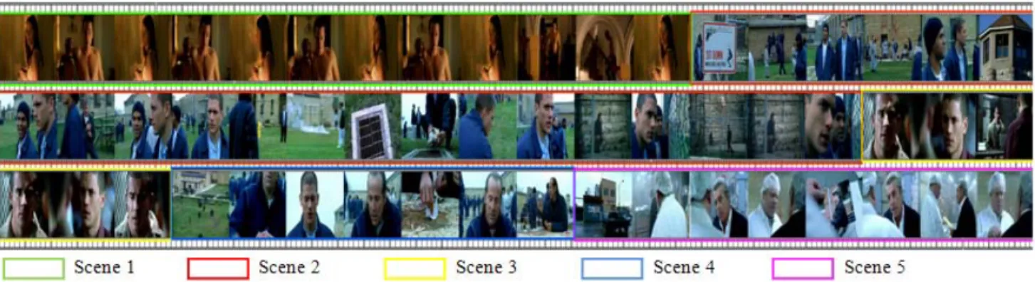
After a complete analysis of the experimental results gathered in Table 5 the following conclusions can be highlighted. The keyframe similarity based on HSV color histogram is generally much faster than SIFT extraction process and can be used when feature detection and matching becomes difficult due to the complete change of the background, important variation of the viewing point, the action development (Fig. 9), etc. The matching technique based on interest points is better suited for scenes that have undergone some great changes but fixed and permanent features are available for extraction and matching. In this case the technique is robust to abrupt changes in the intensity values introduced by noise or changes in the illumination condition etc.

Figure 8. Precision, recall and F1 scorse obtained for different α values

Figure 9. Experimental results obtained after applying our scene segmentation algorithm TABLE V. PERFORMANCE EVALUATION OF THE SCENE EXTRACTION ALGORITHM

Video name Ground truth scenes

SIFT descriptor HSV color histogram

D FA MD _(%) R _(%) P _(%) F1 D FA MD _(%) R _(%) P _(%) F1

Sienfeld 24 19 1 5 95.00 79.16 86.36 20 0 4 100 83.33 90.88

Two and a half men 21 18 0 3 100 81.81 90.00 17 2 4 89.47 80.95 85.01

Prison Break 39 31 3 8 91.17 79.48 84.93 33 0 6 100 84.61 91.66

Ally McBeal 32 28 11 4 71.79 87.50 78.87 24 4 8 84.00 75.00 79.24

Sex and the city 20 17 0 3 100 85.00 91.89 15 1 5 93.75 75.00 83.33

Friends 17 17 7 0 70.83 100 82.92 17 7 0 70.83 100 82.92 5th Element 63 55 24 8 69.62 87.30 77.46 54 10 9 83.05 84.48 83.76 Ace -Ventura 36 34 11 2 75.55 94.44 83.95 29 2 7 92.85 78.78 85.24 Lethal Weapon 4 67 63 39 4 61.76 94.02 74.55 64 25 3 71.97 95.52 82.05 Terminator 2 66 61 11 5 84.72 92.42 88.41 60 7 6 89.55 90.90 90.22 The Mask 44 40 5 4 88.88 90.91 89.88 38 7 6 84.44 86.36 85.39 Home Alone 2 68 56 6 12 90.32 82.35 86.15 57 5 11 90.90 81.96 86.20 TOTAL 497 439 118 58 88.32 78.81 83.29 428 70 69 86.11 85.94 86.02

VI. CONCLUSION AND PERSPECTIVE

In this paper, we have proposed a novel methodological framework for temporal video structuring and segmentation, which includes shot boundary detection, keyframe extraction and scene identification methods. Our contributions concern more specifically an improved, two-step shot boundary detection algorithm, based on scale space filtering of the similarity signal derivatives, a fast keyframe extraction mechanisms, and finally, a reliable scene detection method based on shot clustering and temporal constraints validated using two types of features: HSV color histogram and interest points with SIFT descriptors.

The shot boundary detection methods provide high precision and recall rates (with gains up to 9.8% and 7.4%, respectively in the case all transitions), while reducing with 25% the associated computational time.

Concerning the shot merging into scenes strategy, we have proposed a novel grouping method based on temporal constraints that uses adaptive thresholds and neutralized shots.

The experimental evaluation validates our approach, when using either interest points or HSV color histogram. The F1 measure in both cases is around 86%.

Our perspectives of future work will concern the integration of our method within a more general framework of video indexing and retrieval applications, including object detection and recognition methodologies. Finally, we intend to integrate within our approach motion cues that can be useful for both reliable shot/scene/keyframe detection and event identification.

REFERENCES

[1] Zhang, H.J., Kankanhalli, A., Smoliar, S.W.: Automatic partitioning of full-motion video, Multimedia Systems no. 1 (1993), 10–28.

[2] Lienhart, R., Pfeiffer, S., Effelsberg, W.: Video Abstracting, Communications of the ACM (1997), 1 -12.

[3] Yuan, J., Wang H., Xiao L., Zheng W., Li, J., Lin, F., Zhang, B.: A formal study of shot boundary detection, IEEE Trans. Circuits Systems Video Tech., vol. 17, (2007), 168–186.

[4] Gargi, U., Kasturi R., Strayer, S.: Performance characterization of video shot-change detection methods, IEEE Trans. Circuits and Systems for Video Technology, Vol.CSVT-10, (2000) No.1 1-13.

[5] Zabih, R., Miller, J., Mai, K.: A feature-based algorithm for detecting and classifying scene breaks, Proc. ACM Multimedia 95, (1995) 189– 200.

[6] Porter, S.V., Mirmehdi, M., Thomas, B.T.: Video cut detection using frequency domain correlation, 15th _{International Conference on Pattern}

Recognition (2000) 413–416.

[7] Fernando, W.A.C, Canagarajah, C.N., Bull, D.R.: Scene change detection algorithms for content-based video indexing and retrieval, IEE Electronics and Communication Engineering Journal (2001) 117–126. [8] Hendrickson, B., Kolda, T. G.: Graph partitioning models for parallel

computing, Parallel Computing Journal, Nr. 26, (2000) 1519-1534. [9] Hanjalic, A., Zhang, H. J.: An integrated scheme for automated video

abstraction based on unsupervised cluster-validity analysis, IEEE Transactions on Circuits and Systems for Video Technology, vol. 9, no. 8, (1999).

[10] Fu, X., Zeng, J.: An Improved Histogram Based Image Sequence Retrieval Method, Proceedings of the International Symposium on Intelligent Information Systems and Applications (IISA’09), 015-018. [11] Zhang, H., Wu, J., Zhong, D., Smoliar, S. W.: An integrated system for

content-based video retrieval and browsing, Pattern Recognition., vol. 30, no. 4 (1999) 643–658.

[12] Girgensohn, A., Boreczky, J.: Time-Constrained Keyframe Selection Technique, in IEEE Multimedia Systems, IEEE Computer Society, Vol. 1, (1999) 756- 761.

[13] Aner, A., Kender, J. R.: Video summaries through mosaic-based shot and scene clustering, in Proc. European Conf. Computer Vision, (2022) 388–402.

[14] Rasheed, Z., Sheikh, Y., Shah, M.: On the use of computable features for film classification, IEEE Trans. Circuits Syst. Video Technol., vol. 15, no. 1, (2005) 52–64.

[15] V. Chasanis, A. Likas, and N. P. Galatsanos. Video rushes summarization using spectral clustering and sequence alignment. In

TRECVID BBC Rushes Summarization Workshop (TVS’08), ACM International Conference on Multimedia, pages 75–79, Vancouver, BC, Canada, 2008.

[16] Y. Li, B. Merialdo, “VERT: a method for automatic evaluation of video summaries”, ACM Multimedia; pp. 851-854, 2010.

[17] Hanjalic A, Lagendijk RL, Biemond J, Automated high-level movie segmentation for advanced video-retrieval systems, IEEE Circuits Syst Video Technol 9(1999) 580–588.

[18] Ariki Y., Kumano M., Tsukada K.: Highlight scene extraction in real time from baseball live video. Proceeding on ACM International Workshop on Multimedia Information Retrieval, (2003) 209–214. [19] Ngo C.W., Zhang H.J.: Motion-based video representation for scene

change detection. Int J Comput Vis 50(2), (2002) 127–142.

[20] Chasanis, V., Kalogeratos, A., Likas, A.: Movie Segmentation into Scenes and Chapters Using Locally Weighted Bag of Visual Words, Proceeding of the ACM International Conference on Image and Video Retrieval (CIVR 2009).

[21] Zhu, S., Liu, Y.: Video scene segmentation and semantic representation using a novel scheme, Multimedia Tools and Applications, vol. 42, no. 2, (2009) 183-205.

[22] Lowe, D.: Distinctive image features from scale-invariant keypoints, International Journal of Computer Vision (2004), 1-28.

[23] V. Chasanis, A. Likas, and N. P. Galatsanos. Video rushes summarization using spectral clustering and sequence alignment. In

TRECVID BBC Rushes Summarization Workshop (TVS’08), ACM International Conference on Multimedia, pages 75–79, Vancouver, BC, Canada, 2008.

[24] Y. Li, B. Merialdo, “VERT: a method for automatic evaluation of video summaries”, ACM Multimedia; pp. 851-854, 2010.