Are the Dorsa Argentea on Mars eskers?

HAL Id: hal-02271732

https://hal.archives-ouvertes.fr/hal-02271732

Submitted on 27 Aug 2019

HAL is a multi-disciplinary open access

archive for the deposit and dissemination of

sci-entific research documents, whether they are

pub-lished or not. The documents may come from

teaching and research institutions in France or

abroad, or from public or private research centers.

L’archive ouverte pluridisciplinaire HAL, est

destinée au dépôt et à la diffusion de documents

scientifiques de niveau recherche, publiés ou non,

émanant des établissements d’enseignement et de

recherche français ou étrangers, des laboratoires

publics ou privés.

Are the Dorsa Argentea on Mars eskers?

Frances Butcher, Susan Conway, Neil Arnold

To cite this version:

Frances Butcher, Susan Conway, Neil Arnold. Are the Dorsa Argentea on Mars eskers?. Icarus,

Elsevier, 2016, 275, pp.65-84. �10.1016/j.icarus.2016.03.028�. �hal-02271732�

ContentslistsavailableatScienceDirect

Icarus

journalhomepage:www.elsevier.com/locate/icarus

Are

the

Dorsa

Argentea

on

Mars

eskers?

Frances

E.G.

Butcher

_,

_Susan

_J.

_Conway

_,

_Neil

_S.

_Arnold

a Department of Physical Sciences, The Open University, Walton Hall, Milton Keynes, MK7 6AA, United Kingdom

b Laboratoire de Planétologie et Géodynamique de Nantes, UMR CNRS 6112, 2 rue de la Houssinière - BP 92208, 44322 Nantes Cedex 3, France c Scott Polar Research Institute, University of Cambridge, Lensfield Road, Cambridge, CB2 1ER, United Kingdom

a

r

t

i

c

l

e

i

n

f

o

Article history:

Received 21 December 2015 Revised 11 March 2016 Accepted 31 March 2016 Available online 11 April 2016 Keywords:

Mars

Mars, polar geology Mars, surface Geological processes

a

b

s

t

r

a

c

t

TheDorsaArgenteaareanextensiveassemblageofridgesinthesouthernhighlatitudesofMars.They havepreviously beeninterpreted aseskers formed bydeposition ofsediment insubglacial meltwater conduits,implyingaformerlymoreextensivesouthpolaricesheet.Inthisstudy,weundertakethefirst large-scalestatisticalanalysisofaspectsofthegeometryandmorphologyoftheDorsaArgenteain com-parisonwithterrestrialeskersinordertoevaluatethishypothesis.Theridgesarere-mappedusing inte-gratedtopographic(MOLA)andimage(CTX/HRSC)data,andtheirplanargeometriescomparedtorecent characterisationsofterrestrialeskers.Quantitativetestsforesker-likerelationshipsbetweenridgeheight, crestmorphologyandtopographyarethencompletedforfourmajorDorsaArgentearidges.Thefollowing keyconclusionsarereached:(1)StatisticaldistributionsoflengthsandsinuositiesoftheDorsaArgentea aresimilartothoseofterrestrialeskersinCanada.(2)PlanargeometriesacrosstheDorsaArgentea sup-portformationofridgesinconduitsextendingtowardstheinteriorofanicesheetthatthinnedtowards itsnorthernmargin,perhapsterminatinginaproglaciallake.(3)Variationsinridgecrestmorphologyare consistentwithobservationsofterrestrialeskers.(4)Statisticaltestsofpreviouslyobservedrelationships betweenridgeheightandlongitudinalbedslope,similartothoseexplainedbythephysicsofmeltwater flowthroughsubglacialmeltwaterconduitsforterrestrialeskers,confirmthestrengthofthese relation-shipsforthree offourmajorDorsaArgentea ridges.(5)The newquantitativecharacterisations ofthe DorsaArgenteamayprovideusefulconstraintsforparametersinmodellingstudiesofaputativeformer icesheetinthesouthpolarregionsofMars,itshydrology,andmechanismsthatdroveitseventual re-treat.

© 2016TheAuthors.PublishedbyElsevierInc. ThisisanopenaccessarticleundertheCCBYlicense(http://creativecommons.org/licenses/by/4.0/).

1. Introduction

The DorsaArgentea are an assemblage of_∼7000kmof ridges inthesouthernhighlatitudesofMars(70°–80°S,56°W–6°E).They give theirnametotheDorsaArgenteaFormation(DAF,equivalent totheHesperianpolarunitinTanaka et al. (2014a) inwhichthey arelocated (Fig. 1 ).The DorsaArgentea arethemostextensiveof sevenassemblagesofridgesdistributedthroughouttheDAF(Kress and Head, 2015 ). TheDAF isadjacent to thepresent Amazonian-aged (_< 3.2Ga) (Hartmann, 2005 ) south polar layered deposits (SPLD), comprising water and carbon dioxide (CO2) ice deposits

(Phillips et al., 2011 ). The DAF is distributed in two major lobes centredonthe_∼0°Eand_∼290°Elongitudelines(Ghatan and Head, 2004 ).TheDorsaArgenteatrendSEtoNWwithinthe∼290°EDAF lobewhichextendsto∼65°S,withitsnorthernmostextent

reach-∗ _{Corresponding author. Tel.: + 447824616651.}

E-mail address: [email protected] (F.E.G. Butcher).

ing∼55°S.WithinthemostrecentUnitedStatesGeologicalSurvey (USGS) globalmap of Mars(Tanaka et al., 2014a ), the DAFis in-terpretedasremnantsofice-richdepositsemplacedeitherby cry-ovolcanicflowsoratmosphericprecipitationandsubsequently su-perposedbyathin,periglacially-modifiedmantledeposit.TheDAF isbelievedtorangeinthicknessfromalag-depositveneeroverthe underlyingbedrockinthevicinityoftheDorsaArgentearidges,to ablankethundredsofmetresthicktothesouthandeast(Ghatan and Head, 2004 ).

TheDorsaArgentea occur intheheadward regionofArgentea Planum(Ghatan and Head, 2004 ),abroad,NW-trending,∼975km longbasinintheDAFthatistopographicallyconfinedbythe sur-roundingcrateredhighlands(Tanaka et al., 2014a ),andentera nar-rower ∼40km wide valley at its head. In the central region of their distribution, the ridges generally trend N–NW, diagonal to thelong-axisofthebasin(Fig. 1 ).Here,theyemergefromthe de-posits,whichsuperposeseveralridgestoanincreasingdegree to-wardsthesouth(Head, 20 0 0a; Head and Pratt, 2001 ),anddescend intothebasin,beforeascendingortrackingalongtheslopesonits

http://dx.doi.org/10.1016/j.icarus.2016.03.028

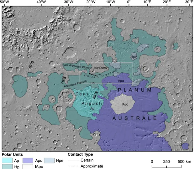
Fig. 1. Map of the south polar region of Mars showing the major surface units ( Tanaka et al., 2014a ) with relevant features labelled, overlain on a hillshade map derived from 460 m/pixel MOLA DEM. The black arrow shows the general trend of the Dorsa Argentea ridges. Ap is the Amazonian polar unit; Apu is the Amazonian polar undivided unit; Hpe is the Hesperian polar edifice unit; Hp is the Hesperian polar unit, equivalent to the Dorsa Argentea Formation (DAF); and IApc is the Late Amazonian polar cap unit. The white box delineates our study area. Projection is south polar stereographic. Surface units, labels and contacts between them are modified from Tanaka et al. (2014a) .

distalside.At theNEmargin ofArgenteaPlanum (Fig. 1 ), several ridgesturneastandenterthenarrow∼550km-longEastArgentea Planum (Ghatan and Head, 2004 ). Individual ridgeshave lengths ofuptoseveralhundred kilometres(Metzger, 1992 )withheights upto120mandwidthsup to6km(Head and Pratt, 2001 ).They rangefromstand-aloneridgestobifurcatingandbraidednetworks (Howard, 1981; Kargel and Strom, 1992 ), andexhibit evidence of superposition(Head and Hallet, 2001a ). Buffered crater counting byKress and Head (2015) returnsabest-fitageof3.48Gaforthe DorsaArgentearidges,correspondingtotheEarlyHesperianperiod ofMars’geologicalhistory.

The DorsaArgenteahavepreviously beeninterpreted as lacus-trine (Parker et al., 1986 ), volcanic (Tanaka and Scott, 1987; Ruff and Greeley, 1990 ),tectonic(Kargel, 1993 ),aeolian(Ruff and Gree- ley, 1990 ),erosional(Ruff and Greeley, 1990; Kargel, 1993; Tanaka and Kolb, 2001; Tanaka et al., 2014b ) or glaciofluvial features (Howard, 1981; Metzger, 1992; Kargel and Strom, 1992; Kargel, 1993; Head, 20 0 0a, 20 0 0b; Head and Hallet, 20 01a, 20 01b; Head and Pratt, 2001; Tanaka et al., 2014b; Kress and Head, 2015 ).

Although manyoftheseinterpretations havealreadybeen ex-cludeddue tomorphological inconsistencieswith terrestrial ana-logues(e.g. Head and Pratt, 2001 , and references therein), a

de-scriptionoftheDorsaArgenteaaseithereskersorinvertedfluvial channelsinthemostrecentUSGSgeologicalmapofMars(Tanaka et al., 2014b ) highlights that a consensus on their originhas not yetbeenreached.

Eskers are ridgesformed by deposition ofglacial sedimentin ice-contact meltwater channels,and subsequent lowering of this materialto,oritsexposureat,thegroundsurfaceduring deglacia-tion (e.g., Banerjee and McDonald, 1975; Brennand, 20 0 0; Benn and Evans, 2010 ). Complex supraglacial, englacial and subglacial drainagewithin terrestrialicesheetsgivesrise toadiverserange of morphologies and configurations of terrestrial esker systems (e.g.,Banerjee and McDonald, 1975; Brennand, 20 0 0; Perkins et al., 2016 ).Relationshipsbetweenridgecross-sectional(CS)dimensions andCS crestmorphologyandthesurroundingtopography,similar tothoseobservedforterrestrialeskers,havebeenidentifiedforthe Dorsa Argentea, and explained using Shreve’s (1972, 1985a ) the-ory onthephysics ofmeltwaterflow throughsubglacial conduits (Head and Hallet, 2001a, 2001b ).

However,nolarge-scalequantitativetestsoftheserelationships have been presented for the ridges and photogeologic analysis to date has largely been limitedto assessment of low-resolution (∼150 to 300m/pixel) images from the Viking Orbiters (e.g.,

Howard, 1981; Kargel and Strom, 1992; Head, 20 0 0b; Head and Pratt, 2001 ).Furthermore,nodetailedstatisticalcharacterisationof planar geometriesofa large sampleof theDorsaArgentea ridges haspreviously beenpresented,perhaps duetoa lackofsimilarly extensive,ice-sheet-scaledatasetsforterrestrialeskeranalogues.

Recent publication ofthe first large-scalequantitative analysis of planar geometries of terrestrial eskers (Storrar et al., 2014a ), formed during deglaciation of the Laurentide ice sheet between 13,000and7000yearsago(Storrar et al., 2014b ),givesanew op-portunity forcomparisonandassessmentof theesker hypothesis fortheDorsaArgentea,whichweexploithere.

Wepresentextensivequantitativecharacterisationofplanar ge-ometriesoftheDorsaArgenteaincomparisonwiththelarge sam-ple of terrestrialeskers analysed by Storrar et al. (2014a) . Addi-tionally,we quantifyCS dimensionsoffourmajor DorsaArgentea ridgesandclassify their crest morphologiesusing high-resolution topographic(MOLA)andmedium-resolutionimage(CTX)datasets, and present the first statistical assessment of esker-like topo-graphic relationshipsforthe DorsaArgenteathat were previously observed by Head and Hallet (2001a) . We therefore present the firstrigorousquantitativestatisticaltestsofthehypothesisthatthe DorsaArgentea aremorphologicallyconsistentwithterrestrial es-kers.Suchassessmentisnecessaryasagrowingbodyofliterature uses theinterpretationoftheDorsaArgenteaaseskersasabasis for inferencesabout the character ofa putative former ice sheet thought to have extended into the DAF during Mars’ Hesperian period, and the nature of its recession (Head, 20 0 0a; Head and Pratt, 2001; Milkovich et al., 2002; Ghatan and Head, 2004; Fas- took et al., 2012; Scanlon and Head, 2015; Kress and Head, 2015 ).

Similaritieshavebeenobservedbetweensubparallelcurvilinear andisolated linear-curvilinear ridgeswithin ridge assemblagesin theCaviAngustiandPlanumAngustumsectorsoftheDAF,and ter-minalmoraines marking theformer extents ofterrestrialglaciers andicesheets(Kress and Head, 2015 ).Ifcorrect, theexistence of moraineridgeshasimplicationsforthe geomorphicrecordofthe formerextentandretreatofaputativeformericesheetintheDAF. However,Kress and Head (2015) acknowledgethatfurther investi-gation of these features is required to test the moraine hypoth-esis. The quantitative description ofthe DorsaArgentea ridgesin the present study may provide useful inputs fortests for differ-encesinmorphologyand, byextension,mechanismsofformation between the Dorsa Argentea and other ridge assemblages in the DAF.

If quantitative and statistical analyses of the Dorsa Argentea and comparison to planar geometries and topographic relation-ships observed for terrestrialeskers support the hypothesis that the Dorsa Argentea are eskers, the quantitative characterisations containedwithinthisstudymayprovideusefulconstraintsfor pa-rameters in modelling studies ofa putative former icesheet ex-tendingintotheDAF,itshydrology,andmechanismsthatdroveits eventualretreat.Alackofsufficientconstraintsupontheterminus position of thisputative ice sheetmeans that, atpresent, recon-structionofglacierthicknessakintothatperformedbyBernhardt et al. (2013) based on ice-surface slopes derived from putative eskers in Argyre Planitia, is not possible for the Dorsa Argen-tea. Identification ofa possible terminusof the putative DAF ice sheet is beyond the scope of the present study, which purely aimstorigorouslytestthehypothesisthat theDorsaArgenteaare eskers.

Furthermore, possible identification of the first martian es-ker connected to its parent glacier in the Phlegra Montes re-gion (Gallagher and Balme, 2015 ) suggests that eskers may be widespreadgeomorphologicalfeaturesdiagnosticofglaciated land-scapesonMars(Kargel and Strom, 1992; Banks et al., 2009; Ivanov et al., 2012; Bernhardt et al., 2013; Erkeling et al., 2014 ).Itis there-forenecessary tobegina quantitative description oftherangeof

characteristicsofputativeeskersonMarstofacilitatetheir identi-fication.

2. Background:terrestrialeskers

Giventhegreatlengths(>100km),lowdegreeoffragmentation (Metzger, 1992 ), location within potential tunnel valleys (Kargel and Strom, 1992 ), and lack of morainic features associated with theDorsaArgentearidgeson Mars(Howard, 1981 ),theterrestrial esker analogues of mostinterest for the presentstudyare those formedwithin subglacialconduits beneatha stagnantorsluggish icemassthatdoesnot overridesedimentarybedformsduring re-treat (Metzger, 1991, 1992; Scanlon and Head, 2015; Kress and Head, 2015 ).

2.1. Planargeometry

Eskersadoptthepathsoftheconduitsinwhichtheyform,and therefore havesimilar configurations and geometries to drainage networksformedduringdeglaciation.Storrar et al. (2014a) present data forthe distributions of length, degree of fragmentationand sinuosityof a large sample(n>20000) ofeskers inCanada. In-dividualCanadian eskerswithlengthsup to 97.5kmform longer fragmentedchainsofeskersupto760kminlength,inwhichgaps account for 34.9 % of the total length. Storrar et al. (2014a) at-tributethesegreatlengthstotime-transgressiveformationin spa-tially and temporally stable meltwater conduits close to the re-treatingmarginoftheLaurentideIceSheet.However,mechanisms allowing synchronous formation ofvery long eskers inlong, sta-ble conduits extending towards the interiorof former ice sheets andterminatinginastandingwaterbodyhavealsobeendescribed inrelationtodetailedfield studiesofCanadianeskers(Brennand, 1994; Brennand and Shaw, 1996; Brennand, 20 0 0 ). Fragmenta-tion of eskers into shorter segments separated by gaps can be an outcome of changes insedimentation conditionsin subglacial conduits (Shreve, 1972; Banerjee and McDonald, 1975; Brennand, 1994, 20 0 0 )and/orpost-depositionalerosion,includingerosionby dynamicice at a retreating ice margin (Brennand, 20 0 0; Storrar et al., 2014a ).

The degree to which eskers diverge from straight paths (sin-uosity) may be an outcome of pressure conditions within the subglacial esker-forming conduits (Storrar et al., 2014a ). Ide-alised water-filled meltwater conduits at the base of an ice sheetorglacier,crossing a hard bed, adoptroughly semi-circular cross-sectionsincisedupwardsinto theoverlying ice(R-channels,

Röthlisberger, 1972 ).At thescale ofan icesheet, thedirectionof subglacial water flow through R-channels is thought to be gov-ernedby thesubglacialhydraulic potential (Shreve, 1972 ). Atany given point within an ice sheet, the hydraulic potential (

φ

φ

ρ

where

ρ

ofthe point andPw is the waterpressure within the ice. Whilst

manyfactors caninfluencePw,a commonsimplifying assumption

(e.g.,Flowers, 2015 ) isthatPw can beassumedto beequaltothe

pressureoftheoverlyingice:

Pw=

ρ

(

)

where

ρ

In-sertingEq. 2 intoEq. 1 ,andrearranginggives:

φ

ρ

(

ρ

ρ

)

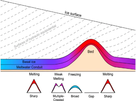
Giventherelativedensities oficeandwater, Eq. 3 showsthat surfacesofhydraulicequipotentialdipup-glacierat∼11timesthe icesurface slope (Fig. 2) (Shreve, 1972 ). These surfaces intersect

Fig. 2. The relationship between esker crest morphology, dimensions and bed topography described by Shreve (1985a) , based on Fig. 5 from Shreve (1985a) and Figure 8.64 from Anderson and Anderson (2010) . Temperature is represented on a gradient from light blue (cold) through to red (warm). Geometries are not accurate and dimensions are exaggerated for clarity. (For interpretation of the references to colour in this figure legend, the reader is referred to the web version of this article.).

thebedwherezequalsthebedelevation(Brennand, 20 0 0 )to pro-ducecontoursofequalsubglacialpotential.Thus,giventhat melt-water flows along the path of the steepest subglacial hydraulic potential gradient(i.e. perpendicular tothe contours ofhydraulic equipotential),theslopeoftheicesurfaceis∼11timesas influen-tialasbedtopographyindeterminingthepathofpressurised wa-terflowinsubglacialconduits,andwatermayascendtopographic features on the bed or track along slopes (Shreve, 1972; Bren- nand, 20 0 0 ),providedthebedslopedoesnotexceed11timesthe icesurfaceslope.Thisissupported byobservations; the_∼150km longterrestrialKatahdin esker systeminMaine USA, ascends to-pographicundulationstoreachelevationsupto∼100mabove sur-roundingtopographiclows(Shreve, 1985a ).Onalevelbed,eskers track in the direction of the steepest ice surface slope (Shreve, 1972; Brennand, 20 0 0 ),formingradial patternsawayfromformer icedivides(Storrar et al., 2014a ).

2.2.Cross-sectionaldimensions,crestmorphologyandrelationships totopography

Eskers adopt the CS dimensions and CS crest morphology of subglacialconduits (R-channels; Section 2.1 ) in which they form, assumingthey completelyfilltheconduits (Banerjee and McDon- ald, 1975; Shreve, 1985a ).Changesinthesepropertiesalongesker profilesare relatedthe physicsof meltwaterflow through water-filled R-channels (Fig. 2 ) (Shreve, 1972, 1985a ). This theory was developed based on the terrestrial eskers of the Katahdin esker systeminMaine,USA,which haveheightsof3-50m,andtypical widthsof150–600m,butcanbeupto2km-wide(Shreve, 1985a ). Thesedimensionsare typicalofmostterrestrialeskers(Clark and Walder, 1994 ),althougheskerscanhaveheightsandwidthsofless than10m(Storrar et al., 2015 ).

R-channelsaremaintainedinasteady-statewhenconduit clo-sureby creepofthesurroundingiceisdirectlyopposedby melt-ingoftheconduitroofandwallsduetoviscousheatingby

melt-water flow (Röthlisberger, 1972 ). However, changes in ice thick-ness andassociatedchanges inthe pressuremelting point(PMP) oficealongconduitpathsdisruptsteady-stateconditions, promot-ing adjustmentofdynamics ofconduit wallmelting andchanges inconduitCS dimensions(Shreve, 1972, 1985a; Anderson and An- derson, 2010 ). Conduits trenddown-glacier into thinner icewith correspondingly higher PMP. Viscous heat produced by frictional interactionofmeltwaterwiththeconduitwallsmustthereforebe partitioned towards warming of waterto the temperatureof the iceintowhichitpassesbeforeoppositionofconduitcreepclosure bywallmeltingcanoccur.

On Earth, on a levelbed, waterwarming consumes ∼30 % of the availableheat energy(Shreve, 1985a ) meaning that _∼70% of viscous heat energyis available for wall melting. On descending bedslopes,down-glacierthinning(andwarming)oftheiceis me-diated, promoting stronger wall melting than on a level bed. In contrast,ongently ascending slopes (<∼1.7timestheicesurface gradient onEarth) wall meltingisweakened asthe overlyingice thins downstreammore rapidly thanover a level bed. On slopes

>∼1.7timestheicesurfacegradient,wallmeltingtransitionsinto a regime of wall freezing asviscous heating cannot compensate for increasesin PMP beneath rapidlythinning ice(Shreve, 1972; Anderson and Anderson, 2010 ).Changesintherateofwallmelting withbedslopethereforedrivechangesintheCSdimensionsof es-kersformingwithinconduits.Theconduitroofexperiencesgreater ratesofmeltingorfreezingthanthesidewallsaswaterincontact withthe roof dissipates energyover a smallersurface area rela-tivetoitsdepth(Shreve, 1985a ).Therefore,conduitheightismore sensitivethan widthtochanges inmelt dynamicsduetobed to-pography,resultinginchangesinconduitshape(Shreve, 1985a ).

Accordingly,asisillustrated inFig. 2 ,terrestrialeskersformed onlevelorgentlydescendingbedslopesmaybecharacterisedby tall,sharpcrest morphology approximating atriangularshape. In areas ascending <∼1.7 times the ice surface slope, weaker roof melting leads to lower, multiple-crested esker crest morphology,

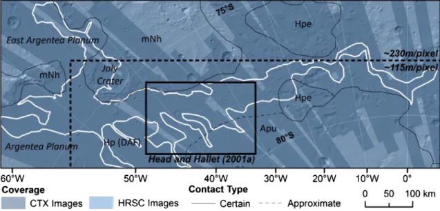
Fig. 3. Data coverage map of the study region (extent displayed in Fig. 1 ) overlain on a hillshade map derived from the ∼460 m/pixel MOLA DEM. The extent of the mapped ridges is outlined in white. The dashed line indicates the boundary between ∼230 m/pixel and ∼115 m/pixel MOLA DEMs. The solid box indicates the approximate study area of Head and Hallet (2001a) . Projection is south polar stereographic. Surface units, labels and contacts are modified from Tanaka et al (2014a) . (For interpretation of the references to colour in this figure legend, the reader is referred to the web version of this article.).

and on steeply ascending slopes (>∼1.7 times the ice surface slope), eskers adopt a lower, broad-crested morphology (Shreve, 1972, 1985a, 1985b; Anderson and Anderson, 2010 ).

Depressionofsurfacesofhydraulicequipotentialatthecrestof topographic undulationsdrives local increasesin thecapacity for sedimenttransportbymeltwater,andmayresultingapsbetween relatedeskersegmentsformingoneithersideofatopographic un-dulationwithinacontinuousconduit(Fig. 2) (Shreve, 1972, 1985a; Anderson and Anderson, 2010 ).Suchsystematicvariationsinridge CSdimensionsandcrestmorphologyhavebeenobservedinan as-semblageofpotential eskersinArgyrePlanitia,Mars(Banks et al., 2009; Bernhardt et al., 2013 ).

3. Methods

3.1. Datasetsandmapping

AllMarsdatawereprojectedinESRIArcMapusingasouth po-larstereographic projection.The latitude ofzerodistortion (stan-dard parallel)wassetto–74.5°S,approximatingthecentreofthe Dorsa Argentea ridge distribution, reducing the estimated mean lineardistortionerrorto± 0.6498%overthestudyarea(seeS1for errorderivation).Wecreatedanimagemosaicprovidingcomplete coverage(Fig. 3 )oftheDorsaArgenteausing∼6m/pixelimagesin the500–800nmwavebandfromtheMarsReconnaissance Orbiter Context Camera (CTX) (Malin et al., 2007 ), with ∼11–20m/pixel panchromatic imagesfrom theMars Express (MEX)High Resolu-tion Stereo Camera(HRSC)(Neukum et al., 2004; Jaumann et al., 2007 ) inCTXdata gaps(Referto TableS2 forlistofimage prod-ucts).Weusedthe∼230m/pixeland∼115m/pixel-resolution grid-ded polar MOLA digital elevation model (DEM) products (Zuber et al., 1992; Som et al., 2008 ) to complement the image data. The ∼230m/pixel DEM was only used to provide coverage of the ridges in the most northerly latitudes of their distribution (Fig. 3 ).MOLAshotdata(PrecisionExperimentDataRecord, MGS-M_MOLA_3_PEDR_L1a-V1.0)were downloadedfromthe PDS Geo-sciencesNodeinshapefileformatandoverlainontheinterpolated DEM toidentifyinterpolatedpixelsintheMOLADEM.Integration of image and topographic datasets improved confidence in

map-pingwhereeithertheimagequality waspoor,orwheretheDEM hadbeeninterpolatedduetoalowdensityofrawaltimetrypoints. Usingthisbasemap,wedigitisedridgesegmentsinArcMapwith polylines following the ridge crest. Segments are defined as in-dividual, unbroken ridges. We conservatively grouped ridge seg-ments into longer ridge systems, defined aschains of ridge seg-ments, separated by gaps, judged to be related on the basis of end-to-endproximity,orientationandvisualsimilarity.Ridgegaps

aredefinedasareasbetweenridgesegmentswhereelevationsare similarto,orlowerthantheadjacentterrain.Segmentsthatcould not be related to systems >10km in length (where distance is linearlyinterpolatedacrossgaps)were excluded fromthe mapas shorterfeatureswere notdistinguishablefromother ’hills’,which canhavesimilaraspectratios.However,thisconservativeapproach inevitably excluded some of the shortest ridges from the map. Mantledridgesextendingnorthwardsfromthegradationalcontact withtheAmazonianpolarunit(Fig. 1 ) wereonlydigitizedifthey formedclearcontinuationofanexposedridgewithintheDAF.

Wheresegments branched orbraided,we usedvisible contin-uation ofridge structure (e.g.layering in sloping sides)from up-ridgeofajunctionto classifyridgecontinuation. Wherebranches weresimilar, weclassifiedthelongestbranchasthecontinuation oftheprimaryridge.

3.2.Planarridgegeometry

As illustrated inFig. 4 ,we extracted thelengths ofindividual ridge segments (segment length, Ls), the total length of all

seg-ments in each ridge system (mapped length, Lm), and the total

lengthofallsegmentsplusthelinearlyinterpolateddistanceacross anygaps(systemlength,Li)fromthemappedpolylines.Gradation

ofsomeridge terminiintothesurroundingterrainintroduced in-accuraciesintheiridentification.Theuncertaintyarisingfrom gra-dationof ridgetermini intothesurroundingterrain was approxi-matedtobe± 44m,whichissignificantlysmallerthanthe distor-tionerrorduetotheprojection(seeS1).

Continuity(C) describesthedegreeofridgefragmentation, de-finedastheratiobetweenLmandLiforeachinterpolatedridge.

Fig. 4. Method for calculation of ridge segment length ( L s ), mapped length ( L m ) and

system length ( L i ). Dots indicate the start and termination points of length calcu-

lations. Gaps in solid lines between points are not included in length calculations. Straight red lines indicate linear interpolation of length calculation across gaps. (For interpretation of the references to colour in this figure legend, the reader is referred to the web version of this article).

Ridgesegmentsinuosity(Ss)isdefinedastheratiobetweenLs

andtheshortestlineardistance(pathlength,Ll)betweentheend

pointsofasegment.Wecalculatedsinuosityofinterpolatedridges

(Si)inasimilarmanner,whereLlwascalculatedbetweenthestart

andendpointsofeachridgesystem.

3.4.Definitionofcross-sectionalprofiles

We sampled fourmajor ridges, arbitrarily namedA-D (Fig. 5 ), foranalysis of the relationship of CS dimensionsand crest mor-phology to topography. These ridges were sampled from the 50 longest interpolated ridge systems. Therefore, cross-sectional ge-ometriesreportedin thisstudylikely reflectthe upperrange for theDorsaArgenteapopulation.Samplingoflongerridgesensured sufficient data for statistically meaningful analyses of individual ridges.Furthermore,iftheDorsaArgenteaareeskers,longerridges arethe mostlikely to haveformed in stableR-channel networks in which conditions most closely approximate the assumptions uponwhichShreve’s (1972, 1985a, 1985b ) theoryisbased.Eskers formedinchannelswheretheassumptions ofShreve’smodelare notmet maynot exhibit the topographicrelationships whichwe soughttotestinthisstudy.Thesampledridgeswerespatially dis-tributedthroughouttheDAF,andthereforeadequatelyrepresented thewholeDorsaArgenteapopulation.

The imagemosaicwasunsuitableforaccurate identificationof theridgebaseduetothegradationofridgesintothesurrounding terrain.Therefore,we obtained_∼6 km-widecross-sectional topo-graphicridgeprofileswithpointspacingsimilartothecellsizeof the∼115m/pixel DEM at∼1kmspacingalong mappedsegments of the sampled ridges for measurement of CS dimensions, crest morphologyandlongitudinalbedslope.CSprofileswerenottaken withinthelower resolution∼230m/pixelDEM.CS profiles where MOLAshotpointdensitieswerelow(fewerthan5shots intersect-ing the ridge within 0.5km of the CS profile) were excluded to minimizethe uncertaintyfromDEMinterpolation. CSprofiles su-perposedonridgegaps,junctions,orimpactcraterswerealso ex-cluded.ElevationvaluesforpointsontheCSprofiles(Z_point)were extractedfromtheMOLADEM.

Fig. 5. Map of the Dorsa Argentea ridges showing the four ridges, A, B, C and D (highlighted) sampled for detailed analysis of cross-sectional dimensions, crest mor- phology and topographic relationships, overlain on a hillshade map derived from ∼115 and ∼230 m/pixel MOLA DEMs and colourised topography, also from these DEMs. Map extent is displayed in Fig. 1 . Black boxes delineate the extents of sub- sequent figures. (For interpretation of the references to colour in this figure legend, the reader is referred to the web version of this article).

Fig. 6. Illustrations of the influence of the textured mantling deposit upon ridges within the study area. (a) CTX image P13_006,282_1046_XN_75S043W overlain with colourised MOLA ∼115 m/pixel DEM showing emergence of Ridge C from textured mantling deposit in the South East. Black box shows location of (b). Extent shown in Fig. 5 (b) CTX image P13_006,282_1046_XN_75S043W of a section of Ridge C close to the contact with the mantling deposit showing remnant accumulations (indicated by black arrows) of the textured deposit adjacent to Ridge C; (c) CTX image P12_005,807_1024_XI_77S035W overlain with colourised MOLA ∼115 m/pixel DEM showing mantling by the textured deposit of ridge intersection A referred to in Fig. 5 of Head and Hallet (2001a) . Extent shown in Fig. 5 . CTX image credit: NASA/JPL-Caltech/MSSS. (For interpretation of the references to colour in this figure legend, the reader is referred to the web version of this article) .

3.5. Cross-sectionaldimensionsandcrestmorphology

Wecalculatedridgeheight(H)andwidth(W)foreachCS pro-filebasedonthegeometryofridgebase(BleftandBright)andcrest

points.Gentlegradationofsideslopesandlocaltopography intro-ducedadegree ofsubjectivityto basepointidentification.To en-sureconsistency, theclassification procedurewasstandardized as follows:

1. CS profile pointswere overlainon the colourised MOLA DEM andcandidatebasepointsselected.

2. Pointswerethen viewedinprofileatfifty-timesvertical exag-geration, and additional candidate base points selected based onbreaksinslope.

3. Candidatepointsidentifiedin(1 )and(2 ) were thenevaluated inplan-viewontheintegratedbasemap, allowing contextuali-sationoftopographyandfinalclassificationofBleftandBright.

We classifiedthe crest asthe highestpoint between Bleft and

B_right.Bedelevation(Z_base) wasapproximatedasthe mean eleva-tion of Bleft (Zl) and Bright (Zr). Ridge height (H) was calculated

asthe difference betweenthe elevationofthe crest point(Zcrest)

andZ_base.Ridgewidth(W)wascalculatedasthedistancebetween

BrightandBleft.

The integrated basemap revealsemergence of Ridge C froma mantlingdepositextendingintotheDAFfromtheAmazonian-aged polar unit in the south (Fig. 6 a) up to 89km along its length. Mann–Whitney U testsfordifference in samplemedians, the re-sultsofwhicharedisplayedinTable 1 ,indicatethatmantledridge sections typically have greater heights and widths than exposed sections. This indicates that CS dimensions and potentially crest

Table 1

Results of preliminary analysis of the effect of the textured mantling deposit upon cross-sectional dimensions of Ridge C using a Mann–Whitney U test for difference between sam ple medians. KS-test is Kolmogorov Smirnov test for nor- mality.

Height , H Width, W

Mantled Exposed Mantled Exposed

n 58 63 58 63 Median (m) 47 36 3667 2669 KS-test value 0.097 0.155 0.072 0.112 KS-test p -value > 0.150 < 0.010 > 0.150 0.049 Mann–Whitney U Wilcoxon value (One-tailed, H1 Mantled > Exposed) 4107 4613 Mann–Whitney U p -value 0.0016 0.0 0 0 0

morphologyaremodifiedsignificantlybythedeposit,andjustifies exclusionofmantledsectionsofRidgeCfromanalysis.Sections af-fectedbyremnantaccumulationsofthemantlingdepositadjacent toRidgeCneartothecontactwiththemantle(Fig. 6 b)werealso excluded.

We classified CS profiles into the sharp, multiple and broad crest morphological types. These categories of crest morphology wereidentifiedbyShreve (1985a) forterrestrialeskers(seeSection 2.2 ). CS profiles withmultiple peaks were classified as multiple-crested.

Sharp and broad crests were distinguished using the criteria of Bernhardt et al. (2013) for putative eskers in Argyre Planitia, Mars,basedonthecross-sectionalslopeatthecrest.Across-ridge

Fig. 7. Examples of classification of ridge crest morphological types. (a) Elevation (coloured lines) and slope (grey lines) profiles are displayed for sharp, broad, and multiple-crested crest morphologies. Letters refer to the start and end points of the profiles displayed in (b) and (c). Scales are equivalent on all three plots and have vertical exaggeration of ∼46. Point spacing along profiles is ∼115 m. (b) A section of Ridge D showing the locations of the sharp-crested and broad-crested cross-sectional profiles in (a). MOLA ∼115 m/pixel DEM overlain on CTX image B08_012,610_1036_XN_76S018W, image credit: NASA/JPL-Caltech/MSSS. Extent dis- played in Fig. 5 . (c) A section of Ridge B showing the location of the multiple- crested cross-sectional profile in (a). MOLA ∼115 m/pixel DEM overlain on CTX im- age G13_023,371_1065_XN_73S048W, image credit: NASA/JPL-Caltech/MSSS. Extent displayed in Fig. 5 . (For interpretation of the references to colour in this figure leg- end, the reader is referred to the web version of this article) .

CSslope(

θ

distancebetweensuccessivepointsalongtheprofile(dMx)andthe changeinelevationbetweenthosepoints(dZpoint).Asillustratedin

Fig. 7 , CS profiles were classifiedas broad-crested where

θ

<1° for three or more consecutive points (>∼345m), including thecrest point,accountingfor>10% ofthe averagewidthof the sampledridges.Single-crestedprofileswithcrestslopes_>1°,were classifiedas sharp-crested. Profiles of Zpoint viewed alongside

θ

profiles(Fig. 7 )confirmedeffectivedistinctionbetweenvisibly dif-ferentcrest morphologicaltypes underthisclassification scheme. Itshould beemphasisedthat thesethresholdcriteriamaynotbe directly applicable to terrestrialeskers, since differencesin vari-ablessuch asgravitybetweenEarthandMarsarelikely toresult invariationsinthevertical expressionoftheridge crests,andby extension,thegeometrythatdefinesthethresholdbetween ‘sharp-crested’and‘broad-crested’eskersections.Giventhatclassification of crest morphology in the present study is not undertaken for thepurposeofcomparingtherawgeometriesofsharp-crestedand broad-crestedsectionstothoseonEarth,butinsteadfortestingfor esker-likedifferencesinbedslopesoccupiedbysharp-crestedand broad-crestedsectionsofthe DorsaArgentea,we considerthisto beanappropriateapproach.

3.6.Longitudinalchangeinridgeheightandbedslope

In order to test the relationship between the change inridge heightandlongitudinalbedslopeobservedby Shreve (1985a) for terrestrialeskers,wecalculatedthedifferencebetweentheheight of each CS profile (H1) and the height of the neighbouring

up-Table 2

Estimations of uncertainties for calculated quantities based on propagation of errors for the most extreme val- ues in the dataset (see S1 for derivation).

Quantity Error Segment length, L s ± 973 m Mapped length, L m ± 5149 m System length, L i ± 5168 m Continuity, C ± 0.02 Segment sinuosity, S s ± 0.01 System sinuosity, S i ± 0.03

Ridge base elevation, Z base ± 0.707 m

Height, H ± 1.23 m

Width, W ± 141 m

Longitudinal change in ridge height, dH ± 1.74 m

Longitudinal bed slope, θL ± 0.1 °

ridge CS profile (H0), dH.We did not perform calculationsof dH

across ridge intersections aschanges in ridge dimensions across eskerjunctionsmaybeinfluencedbyexternally-drivenchangesin meltwaterdischargeata conduit confluence,potentiallyreducing theclarityofanyinternally-controlledrelationship thatmayexist ifthe Dorsa Argentea are eskers. We applied the sameexclusion foranalysisofrelationshipsofcrestmorphologytotopography.

Wecalculatedlongitudinalbedslope(

θ

each CS profile andthe preceding(up-ridge) CS profilebased on the down-ridge changein Z_base (dZ_base) and thelongitudinal dis-tance(dML)betweenthem.Ascendingslopesareindicatedby

pos-itive

θ

The assumption of a consistent bed slope between sampled CS profilesmayhaveoverlookedsub-kilometre-scalevariationsin bedslope.However,the∼1kmspacingbetweenprofiles,whichis smallrelativetothetypicalwidthsofthesampledridges,islikely to have captured the basiccharacteristics of the surrounding to-pography,whichhaslowlevelsofrelief.

3.7. Uncertainties

Uncertaintiesinmeasuredvariablesarisingfromknown instru-mentinaccuracies, experimentallyestimateddistortionduetothe projection,andmethodologicaluncertaintieswerecalculatedbased onpropagationoferrorsforthemostextremevaluesinthedataset andaredisplayedinTable 2 .SeeSupplementaryMaterial(S1)for theirderivation.

4. Results

4.1. Planarridgegeometry

Intotal,wemapped∼6772kmofridgesegments(n=720). De-scriptivestatisticsforsegmentlength(Ls),mappedlength(Lm)and

systemlength(Li)aredisplayedinTable 3.

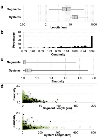
ThedistributionofLs(Fig. 8 a)ispositivelyskewed,varying by

three orders of magnitude from ∼0.2km, up to a maximum of ∼150km,withmedian_∼4.8kmandmean_∼9.4km(Standard Er-ror,S.E.=495m).Log-transformedLsvalues(log10Ls)haveanormal

distribution(Kolmogorov–Smirnov,KS-value=0.03;p-value=0.05) (Table 3 ).Segmentslessthan10kminlengthaccountfor_∼27%of totalLm,whilst thoseexceeding 50kminlength account for∼17

%.Onemappedsegmentexceeds 100kminlength(∼150km), ac-countingfor_∼2%oftotalLm.

When considered as fragments of longer ridge systems (n=206), the mapped ridgesform a total Li of ∼7514km (Table 3 ).Ridgesystems extendup to∼314kminlength. Theminimum recorded length of 10km is likely an artefact of the 10km Li

Table 3

Descriptive statistics of planar geometry of mapped ridges.

Segment length, L s Mapped length, L m System length, L i Continuity, C Segment sinuosity, S s System sinuosity, S i

n 720 206 206 206 720 206 Total 6772 km 6772 km 7514 km NA NA NA Minimum 0.18 km 8 km 10 km 0.59 1.00 1.01 Maximum 150 km 260 km 314 km 1.00 1.75 1.91 Median 4.81 km 20 km 22 km 0.94 1.02 1.07 Mean 9.41 km 33 km 36 km 0.91 1.04 1.10 Standard error 0.495 km 2.483 km 2.764 km 0.01 0.00 0.01 Standard deviation 13.28 km 35.63 km 40 km 0.10 0.06 0.12 Skewness 4.10 3.30 3.37 –1.06 4.98 3.34 Kurtosis 29.29 16.57 18.92 3.51 36.80 14.25 KS-test value 0.24 0.246 0.253 0.171 0.284 0.216 KS-test p -value < 0.010 < 0.010 < 0.010 < 0.010 < 0.010 < 0.010

Log 10 KS-test value 0.03 0.093 0.096 0.185 0.266 0.186

Log 10 KS-test p -value 0.05 < 0.010 < 0.010 < 0.010 < 0.010 < 0.010

Fig. 8. Distributions of planar geometries of the Dorsa Argentea: (a) boxplots of segment length, L s ; and system length, L i , on a log 10 x -axis. Boxes indicate the up-

per and lower quartiles and vertical lines within boxes are median values; (b) his- togram of continuity, C (bin width is 0.1) for ridge systems ( n = 206); (c) boxplots of segment sinuosity, S s and system sinuosity, S i , on a linear x -axis. Boxes indicate

the upper and lower quartiles and vertical lines within boxes are median values; (d) scatterplots of segment sinuosity, S s versus segment length, L s and system sinu-

osity, S i versus system length, L i , (points) overlain on values for the Canadian eskers

(crosses) from ( Storrar et al., 2014a ).

theexistenceofsignificantlyshorterridgeforms.L_iisstrongly pos-itively skewedwith median∼22kmand mean∼36kmwith S.E. 2764m.

Aratioof0.91betweentotal Lm andtotalLiindicates thatthe

DorsaArgentea havelow degreesoffragmentation, withgaps ac-countingfor∼10 %ofLi.Onaverage,eachridgesystemisformed

of3.5(standarddeviation,S.D.=3.2)segments.Thedistributionof continuity (C) values forridge systems (Fig. 8 b) is strongly neg-atively skewed with a median of 0.94 (Table 3 ). Ridge systems formedofa singlesegment(C=1) account for∼30% ofmapped ridges.However, someridge systemshavehigherdegreesof frag-mentation,withaminimumcontinuityof0.59.

In the following description, system sinuosity (Si) is

re-portedwithsegmentsinuosity (Ss) inbrackets.Asissummarised

in Table 3 and shown in Fig. 8 c, the Dorsa Argentea typi-cally have low sinuosities ranging from near-linear with sin-uosity 1.01 (1.00), to paths with sinuosity up to 1.91 (1.75). With a median of 1.02 and mean 1.04 (S.E.₌0.00), Ss is more

stronglypositivelyskewed(skewness=4.98;kurtosis=36.80)than

Si (skewness=3.34; kurtosis=14.25), with a median of 1.07 and

mean1.10(S.E.=0.01).Scatterplotsofsinuositiesagainstridge seg-mentandsystemlengthsinFig. 8 dillustrate thatlong ridgesare typically straighter than shorterridges. A map ofSi, displayedin Fig. 9 aillustratesthatridge systemsattheentrytoEastArgentea PlanumhavehigherS_ivalues(_∼1.48to_∼1.7)thanthosewithinthe mainvalley(∼1to∼1.3).ThiscontrastcanbeseeninFig. 9 b.

4.2.Cross-sectionaldimensionsandcrestmorphology

Assummarized inTable 4 , thefourmajor ridge systems sam-pledfromtheDorsaArgentea(Fig. 5 )rangebetween1and107m in height, with equivalent mean and median heights of 42m (S.E₌1m).The heightsoftheridgeshavea range,onaverage,of 73m(S.E.=9m)alongtheirlengths.

Ridge width ranges between ∼700m and ∼6000m, with a mean width range of _∼4400m (S.E.₌180m) along individual ridges, and mean and median widths of ∼3000m (S.E.=83m) and∼3100m,respectively.Longitudinalvariationsinridge widths are gradual. Ascatterplot of ridge height andwidth displayedin

Fig. 10 showsthat thereis a significant positivelinear correlation betweenheight andwidthwithaPearson’s correlationcoefficient of0.76(p-value=0.00).

The CS profiles sampled from Ridges A, B, C and D (n₌211) aredominatedbysharpcrestmorphologies(75%),withbroadcrest morphologiesaccountingfor24 %.Multiple-crested morphologies account for _<1 % (n₌2) of CS profiles and are excluded from further analysis. Owing to the small number of CS profiles with broad crest morphologies identified on individual ridges (three withn_<15),wecompletedstatisticaltestsfordifferenceinCS di-mensionsbetweensharp-andbroad-crestedCSprofilesforthe en-tiresample,ratherthanforindividualridges.

A one-tailed Mann-Whitney U test for difference in median heights(48m and30m forsharp andbroad crest morphologies, respectively) (Table 5 ) indicates that sharp crest morphologies

Table 4

Descriptive statistics of cross-sectional dimensions of cross sectional profiles on ridges A, B, C and D.

Ridge A Ridge B Ridge C Ridge D All CSPs

n 29 29 63 90 211 Height, H Minimum (m) 21 7 1 8 1 Maximum (m) 77 71 75 107 107 Median (m) 50 28 36 47 42 Mean (m) 48 32 37 48 42 Standard deviation (m) 17 13 23 20 21 Standard error (m) 3 2 3 2 1 Skewness –0.68 0.98 0.98 0.65 0.31 Kurtosis –1.44 2.02 2.020 0.58 –0.18 KS-test value 0.190 0.143 0.155 0.155 0.051 KS-test p -value < 0.010 0.132 < 0.010 < 0.010 > 0.150

KS-test interpretation Not Normal Normal Not Normal Not Normal Normal

Histogram distribution Bimodal Normal Bimodal Bimodal Bimodal

Width, W Minimum (m) 1124 1446 669 1114 669 Maximum (m) 5132 5812 5143 5999 5999 Median (m) 3552 2917 2669 3453 3143 Mean (m) 3425 3410 2516 2957 3083 Standard deviation (m) 1115 1272 1048 906 1203 Standard error (m) 207 236 132 96 83 Skewness –0.68 1.11 0.08 0.02 0.14 Kurtosis –0.39 0.98 –0.82 –0.90 –0.61 KS-test value 0.115 0.147 0.112 0.098 0.063 KS-test p -value > 0.150 0.106 0.049 0.040 0.045

KS-test interpretation Normal Normal Not normal Not normal Not normal

Histogram distribution Normal Normal Bimodal Bimodal Bimodal

Table 5

Descriptive statistics, and Mann–Whitney U tests for difference between sample medians, in ridge height, H , width, W and width–height ratio between sharp and broad crest morphological types on ridges A, B, C and D.

Height Width Width:Height

Sharp Broad Sharp Broad Sharp Broad

n 159 50 159 50 159 50 Minimum (m) 8 1 781 669 32 51 Maximum (m) 99 107 5999 5448 176 721 Median (m) 48 30 3229 2904 69 101 Mean (m) 46 30 3157 2846 74 136 Standard deviation (m) 20 20 1174 1295 24 124 Standard error (m) 2 3 93 183 2 18 Skewness 0.13 1.31 0.15 0.23 1.02 3.29 Kurtosis –0.39 3.44 –0.51 –0.92 1.55 11.35 KS-test value 0.059 0.132 0.066 0.098 0.101 0.351 KS-test p -value > 0.150 0.036 0.088 > 0.150 < 0.010 < 0.010

KS-test interpretation Normal Not Normal Normal Normal Not Normal Not Normal

Mann–Whitney U Wilcoxon Value (One-tailed, H 1 Sharp > Broad) 18,552 NA NA

Mann–Whitney U Wilcoxon Value (One-tailed, H 1 Sharp < Broad) NA NA 14,399

Two-tailed t-test t-value (Assuming unequal variances) NA 1.51 NA

Mann–Whitney U p -value 0.0 0 0 NA 0.0 0 0

Two-tailed t -test p -value NA 0.134 NA

typically have greater heights than broad crest morphologies, returningaWilcoxonvalueof18,552(p-value=0.00).

In contrast, a two-tailed t-test (unequal variances) for normally-distributed widths indicates no significant difference in width between sharp (mean=∼3200m; S.E.=93m) and broad (mean=∼2800m; S.E.=183m) crest morphologies, re-turning a t-value of1.51 which is insignificant atthe 95 % level (p-value=0.134)(Table 5 ).

ThesedifferencesindimensionsareillustratedinFig. 10 which indicatesthatsharp-crestedridgesectionsaregenerallytaller rel-ativetotheirwidthsthanbroad-crested sections,withdifferences inwidth-heightratios(Table 5 ) primarily arisingfromdifferences inheightbetweencrestmorphologicaltypes.Significantdifference indimensionsbetweensharpandbroadcrest morphologies, illus-tratedinFig. 10 ,confirmstheclassificationcriteriamadea mean-ingfuldistinctionbetweencrestmorphologicaltypes.

4.3. Topographicrelationships

The ridges commonly ascend topographic undulations up to ∼100mhigh(e.g.RidgeD,Fig. 11 ).Fig. 11 showsthatincreasesin bedelevationalongridgeprofilesaregenerallyassociatedwith de-creasesinridgeheightandviceversa,asnotedbyHead and Hallet (2001a) .

SimplebivariateplotsofdHand

θ

Pearson’s correlation coefficients of −0.691 (p-value=0.000) and –0.770(p-value=0.000) forRidgesAandB, respectively,indicate that theseridgesstronglyadhere tothe negativecorrelation pre-dictedbyShreve (1972, 1985a )forterrestrialeskers,withincreases inridgeheightondownhillslopes anddecreasesonuphillslopes. RidgesCandDexhibitweakernegativecorrelationswithPearson’s correlation coefficientsof–0.427(p-value=0.001)and–0.324 (p -value=0.003)respectively.

Fig. 9. (a) Map of the Dorsa Argentea classified by system sinuosity, S i overlain on a

hillshade map derived from ∼115 and ∼230 m/pixel MOLA DEMs. Map extent is dis- played in Fig. 1 . (b) ∼115 and 230 m/pixel MOLA DEM overlain on image from the ∼100 m/pixel THEMIS Day IR v11 512ppd global mosaic from USGS (image credit: NASA/JPL-Caltech/Arizona State University) showing a region of the Dorsa Argen- tea. Extent displayed in (a). (c) Map of a region of the terrestrial eskers in Canada mapped by Storrar et al., (2013) , to which the Dorsa Argentea are compared in this study. The scale is similar to that in (a). The reader is referred to the web-version of this article for interpretation of the colours in this figure.

We completed univariate ordinary least squares (OLS) regres-sionanalysesof

θ

vari-able)foreachoftheridges;theresultsaredisplayedinTable 6 .

θ

explains47.81%(p-value=0.000)and59.26%(p-value=0.000)of thevarianceindHalongridgesAandB,respectively.

θ

rela-tivelyweakpredictorofdHalongridgesCandD,explaining18.27 % (p-value=0.001) and 10.47 % (p-value=0.003) of its variance, respectively.RegressionmodelswereevaluatedusingtheMoran’sI statisticaltestforspatialautocorrelation,andaKS-testfor normal-ity,inregressionresiduals(Table 6 ).Wecomputedspatialweights matricesforthe Moran’sItest on thebasis oftheEuclidean dis-tancetothecentroidsofthetwonearestneighbouringCSprofiles. Ridges A, B, C andD do not have statistically significant spatial autocorrelationandexhibit normalityintheir residuals,indicating robust model performance. Non-normality inregression residuals forRidgeDinvalidates thismodel,indicating thatother unidenti-fiedvariablesarerequiredtoexplainvarianceindHforthisridge. TherelativelystrongtopographicrelationshipsobservedforRidges AandBjustifycloserassessmentofthecharacteroftheseridges.

Ridge A (Li=∼47km) passes northwest through an infilled

(_∼10km diameter) crater, traversing topographic lowsin the de-gradedcraterrim,asshowninFig. 13 a.Thetopographicprofileof thecrestofthecraterriminFig. 13 bintersectstheridgebetween sampledCS profiles at∼8km,ontheNW rim, andindicates that theridgemayhaveagapthatwasundetectedinthesystematicCS profilesample,reducingtoanegligibleheightasitpassesoverthe

Fig. 10. Scatterplot of height, H against width, W, for ridge cross-sectional pro- files, classified by crest morphological type. Error bars display uncertainties from Table 2 .

Fig. 11. Longitudinal plots of ridge height, H (coloured lines and points) and base elevation, Z base (grey lines) derived from systematically sampled cross-sectional pro-

files on Ridges A, B, C and D. Gaps in ridge height profiles indicate gaps between ridge segments and points represent ridge segments along which a single cross- sectional profile was sampled. The profile for Ridge C includes the section mantled by the textured deposit (0–89 km) that is excluded from quantitative analysis. Note the different x - and y -axis scales. (For interpretation of the references to colour in this figure legend, the reader is referred to the web version of this article).

Table 6

Ordinary least squares (OLS) regression analyses of longitudinal bed slope θL (independent variable) and longitudinal change in ridge height,

d H (dependent variable) for ridges A, B, C and D: tests of assumptions, results and tests of model performance.

Ridge A ( n = 28) Ridge B ( n = 20) Ridge C ( n = 55) Ridge D ( n = 80)

Test of assumption of normality of dependent variable, dH. (P-value ≥ 0.01 is normal)

KS-test value 0.117 0.135 0.134 0.106

P -value > 0.150 > 0.150 0.021 0.034

Assumption of normality Valid Valid Valid Valid

Model

R -squared 47.81% 59.26% 18.27% 10.47%

F -statistic 23.82 26.19 11.85 9.12

P -value 0.0 0 0 0.0 0 0 0.001 0.003

Bed slope Constant Bed slope Constant Bed slope Constant Bed slope Constant

Coefficient –14.28 –2.47 –20.34 0.23 –9.29 –0.807 –14.60 –0.60

S.E. (Coefficient) 2.93 1.83 3.97 1.02 2.70 0.992 4.83 1.64

T -value –4.88 –1.35 –5.12 0.22 –3.44 –0.81 –3.02 –0.36

P -value 0.0 0 0 0.189 0.0 0 0 0.826 0.001 0.420 0.003 0.716

Significantly different from zero? Yes No Yes No Yes No Yes No

Tests of model performance

Moran’s I test for spatial autocorrelation in OLS regression residuals (k-nearest neighbours, k = 2 )

Moran’s I statistic –0.482 1.017 –1.895 –1.947

P -value 0.630 0.309 0.058 0.052

Spatial autocorrelation? No No No No

Test for normality of regression residuals (P-value > 0.01 is normal)

KS-test value 0.167 0.154 0.075 0.125

P -value 0.046 > 0.150 > 0.150 < 0.010

Normality of regression residuals? Yes Yes Yes No

Fig. 12. Scatterplots of longitudinal change in ridge height (dH) against bed slope ( θL ) for cross-sectional profiles on Ridges A ( n = 28), B ( n = 20), C ( n = 55) and D

( n = 80), with linear trend lines. Upper left quadrants represent descending slopes and increasing ridge heights, and lower right quadrants represent ascending slopes and decreasing ridge height. Error bars display uncertainties from Table 2 .

Table 7

Descriptive statistics for, and tests for difference between, longitudinal bed slopes occupied by sharp and broad crest morphologies.

Sharp Broad n 145 37 Minimum ( °) –1.19 –1.25 Maximum ( °) 0.9882 1.47 Median ( °) –0.03 –0.03 Skewness –0.36 –0.03 Kurtosis 0.92 3.98 KS-test value 0.066 0.189 KS-test p -value 0.129 < 0.010

KS-test interpretation Normal Not normal

Mann–Whitney U Wilcoxon value (two-tailed) 13,254

Mann–Whitney U p -value 0.964

crest.The ridgeiswelldeveloped(H_{≈ 50}m) overthemore sub-duedtopographyoftheSErim(∼22kmalongprofile).Infillingof small(sub-kilometre-scale)cratersinCTXimagesindicatepossible mantlingoftheridgebyadeposit(Fig. 13 a)whichmaydistortthe true dimensions and topographic relationships of the underlying ridge.However, surfacemanifestationoftherimsofsmallinfilled craters indicates that this deposit is thinner than that mantling ridgesinthe south(Section 3.5, Fig 6 ) andmaythereforehavea morelimitedeffectuponthedimensionsoftheunderlyingridge.

RidgeBisthelongestofthemappedridgesystemsoftheDorsa Argentea(Li=314km)andappearstobeunaffectedbythedeposit

thatmantlesRidgeA.Itistheprimary ridgepassingintoEast Ar-genteaPlanum from themain valley, NW ofJoly Crater, andhas two major tributary ridge systems,forming a branching network (Fig. 14 a). Closeto theentrytoEastArgentea Planum,a pedestal feature,showninFig. 14 a,extendslaterallyfromanouterbendin theridge.CTXimagesreveallayeringintheslopingsidesofsome ridgesections(Fig. 14 b),whichmaybecontinuousoverdistances ofkilometres.

Equivalentmediansof–0.03° indistributionsofbedslopes oc-cupied by sharp and broad crest morphologies indicate no dis-cernibledifferenceinbedslopesoccupiedbysharpandbroadcrest morphological types. This is confirmed by a two-tailed Mann– WhitneyUtest,(Table 7 )whichreturnsastatisticallyinsignificant Wilcoxonvalueof13,254(p-value=0.964).

Fig. 13. (a) Passage of Ridge A through an infilled crater (CTX images B12_014_285_1025_XN_77S026W and B12_014,351_1024_XN_77S028W, image credit: NASA/JPL- Caltech/MSSS). Image extent is displayed in Fig. 5 . (b) Topographic profile of the crater rim derived from the ∼115 m/pixel MOLA DEM, passing anticlockwise from the point marked in (a). Points on the profile that intersect Ridge A are indicated with vertical arrows.

5. Analysis

5.1. ComparisontopreviousstudiesoftheDorsaArgentea

The lengths of the longest ridge systems mapped in the present study are consistent with the upper length range (hun-dreds of kilometres) identified for the Dorsa Argentea by pre-vious workers (Howard, 1981; Metzger, 1992; Head and Pratt, 2001 ). Whereas previous assessments of planar geometries of the Dorsa Argentea have primarily been dependent upon low-resolution(∼150–300m/pixel)VikingOrbiterimages,theinclusion of higher-resolution CTX images in the integrated basemap em-ployed within the present study allows greater insight into the influence of shorter ridge systems upon the statistical distribu-tion of ridgelengths. The meaninterpolated length ofridge sys-tems in the Dorsa Argentea fromthe present study(∼37km) is shorter thanthe lower-bounding length (∼50km) ofthe shortest ridgesidentifiedbyHead and Pratt (2001) andsignificantlyshorter than the mean length of 153km stated by Metzger (1992) for the Dorsa Argentea and putative eskers in Argyre Planitia, combined.

The highcontinuity (mean=0.91, S.E.=0.01)of theridge sys-tems mapped in the present study is similar, though slightly

lower, than the average continuityof 0.97 measured by Metzger (1992) using _∼150–300m/pixel Viking images. This may be at-tributed to the higher resolution of images employed in the present study, which allowed better identification of ridge gaps. Mean system sinuosity (1.10, S.E.₌0.01) is consistent with the valueof1.2obtainedbyMetzger (1992) .AlthoughKress and Head (2015) donotdefine whethertheir calculationsofridgesinuosity, whichare basedon higher-resolutiondatathan thoseofMetzger (1992) , are based on ridge segments or interpolated ridge sys-tems, their value of mean sinuosity (∼1.06) falls between those values(1.04and1.10,respectively)calculatedinthepresentstudy, improvingconfidencein theresults.However, whereas Kress and Head (2015) assertthat,onaverage,longerridgesintheDorsa Ar-genteahavehighersinuosity,plotsofridgesegmentsinuosityand ridge system sinuosity against ridge length in the present study (Fig. 8 d)indicatethatlongerridgesgenerallyhavelowersinuosity thanshorterridges.

The ridges sampled in the present study have heights up to 107m and widths up to ∼6km, towards the upper range of di-mensionsidentifiedbypreviousworkers(Head and Hallet, 2001b; Head and Pratt, 2001 ).Duetosamplingofthelongestridges,CS di-mensionspresentedhere(Table 4 )likelyrepresenttheupperrange fortheDorsaArgenteapopulation.

Fig. 14. (a) Image from ∼100 m/pixel THEMIS Day IR v11 512ppd global mosaic from USGS (image credit: NASA/JPL-Caltech/Arizona State University) of a section of Ridge B (extent displayed in Fig. 5. ) showing the lateral pedestal feature (out- lined). Black arrows indicate entry of Ridge B into East Argentea Planum. The black box shows the extent of (b). (b) Evidence of layering structures in the side slopes of Ridge B (CTX image G13_023 371_1065_XN_73S048W, image credit: NASA/JPL- Caltech/MSSS). (For interpretation of the references to colour in this figure legend, the reader is referred to the web version of this article).

Previous work has shown that the Dorsa Argentea do not consistently follow the steepest topographic slope. Instead, they track along slopes and occasionally ascend topographic undula-tions (Howard, 1981; Head and Hallet, 20 01a, 20 01b ). In a brief conference abstract that focussed on the relatively small region of the Dorsa Argentea demarcated in Fig 3, Head and Hallet (2001a) identifiedtendencies forincreasesinridge height on de-scendingslopesanddecreasesinridgeheightonascendingslopes, consistent with formation in pressurised subglacial conduits (Shreve, 1985a; Head and Hallet, 2001b ).OLSregressionmodelsof percentagelongitudinalchange inridge height andbedslope for two ofthe sampledridges(Table 6 ) providequantitative statisti-calsupportfortheseobservations.Sharp,multipleandbroadcrest morphologicaltypesidentifiedwithinthepresentstudyare consis-tentwiththetype1,2and3ridgemorphologicaltypesidentified byHead and Hallet (2001a) fortheDorsaArgentea.However, pref-erential occurrenceof multiple andbroad crest morphologies on ascendingslopes,comparedtosharpcrestmorphologiesinregions oflow regionalslope,asidentifiedbyHead and Hallet (2001a) ,is notsupported bythequantitativeanalysispresentedhere.No dis-cernibledifferenceisfoundbetweenbedslopesoccupiedbyridge sectionswithsharpandbroadcrestmorphologies. Thedifference betweenour findings,andthose ofHead and Hallet (2001a) may becausedbythethresholdcriteriaselectedinthisstudyto distin-guishbetweensharp andbroadcrest morphologies. It could also showthattherelationshipisweakerthanthatstudysuggests.CTX imagesreveal a textured depositwhich extends from the grada-tional boundary of the Amazonian polar undivided unit (Tanaka

et al., 2014a )andmantlesthespecificridgesectionstowhichHead and Hallet (2001a) refer (Fig. 6 c). This mantlesignificantly alters the dimensionsof the ridges(Table 1 ) and mayalso affect their crest morphology. Drapingof thismantle over underlying topog-raphymaybroadenthesurfaceexpressionoftheunderlyingridge asitpassesover atopographic obstacle,particularlyifthat topo-graphicobstacleisorientedperpendiculartothepathoftheridge, asintheexampleusedbyHead and Hallet (2001a) (Fig. 6 c).This suggeststherelationshipbetweenridgecrestmorphologyandbed topographyfortheDorsaArgenteamaynotbeasstrongas previ-ouslysuggested.

5.2. Previouscomparisonstoterrestrialeskeranalogues

ComparisonsofplanargeometriesoftheDorsaArgenteato ter-restrialeskeranalogueshavepreviouslybeenlimitedbyapaucity ofquantitative datafora large (ice-sheet-scale)sampleof terres-trial eskers. As a result, previous studies have been limited to comparison of geometries of the Dorsa Argentea to simple de-scriptions of planar geometries of relatively small esker assem-blagessuchasanassemblageof130eskersinNewYorkState,USA (Metzger, 1992, 1991; Kargel and Strom, 1992 ),and theKatahdin eskersysteminMaine,USA(Kargel and Strom, 1992; Head, 20 0 0a; Head and Hallet, 2001a, 2001b; Head and Pratt, 2001; Kress and Head, 2015 ),whichcomprisesonemajoreskerwithfivetributaries (Shreve, 1985a ).

Metzger (1991, 1992) identified similarities in sinuosity be-tweenterrestrialeskersinNewYorkState,USAandtheDorsa Ar-gentea.Thesesimilaritieshavemorerecentlybeencorroboratedby

Kress and Head (2015) . However, Metzger (1991, 1992) acknowl-edgethattheloweraveragelength(∼8.2km)andcontinuity(∼64 %)oftheseterrestrialeskers,relativetotheDorsaArgentea,limits theirapplicabilityasanalogues.

In a comparison to morphological descriptions by Brennand (20 0 0) of eskers formed beneath the Laurentide IceSheet, Kress and Head (2015) support similaritiesin plan-view map patterns, dimensions and sinuosity between long, sinuous andcontinuous ridgesof the DorsaArgentea and terrestrialeskersformed in ef-ficient channelised subglacial drainage conduits (R-channels, see

Section 2.1 ).

However, they also distinguish a second population of ridges in the Dorsa Argentea which are shorter (kilometres to tens of kilometres in length) and more polygonal in their configuration than the long, sinuous and continuous ridges, and occur in re-gionsbetweenthem.Theyproposethattheseridgeswere formed by deposition in less efficient, ‘slow’ drainage systems (Fountain and Walder, 1998 ) in inter-R-channel areas ofthe bed. In ‘slow’, or‘distributed’ drainage networks, waterflows along narrow ori-ficesbetweenlinkedbasalcavitieswhichformasaresultofglacial flowover topographicirregularities inthebed(Kamb, 1987 ). Ter-restrialanaloguesforeskersformedindistributedsystemsdonot exist,sinceeskers,bydefinition,forminchanneliseddrainage sys-tems rather than distributed systems. The most similar terres-trial eskers to which Kress and Head (2015) refer are shortand deranged type III eskers as classified by Brennand (20 0 0) . The drainagesystemsinwhichtheseeskersformarecharacterisedby short R-channels draining into interior lakes or channels incised intothe bed(Brennand, 20 0 0 ),andare thereforedifferent tothe distributednetworksinwhichKress and Head (2015) proposethe shorter,polygonalridgesoftheDorsaArgenteaformed.

Therecentsurvey byStorrar et al. (2014a) of_>20000 terres-trial eskers in Canada provides the most extensive and detailed quantitativecharacterisationofterrestrialeskerstodate.This pro-vides a newopportunity formore detailedquantitative compari-sonofplanargeometriesoftheDorsaArgenteatoterrestrialesker analogues. Although itis possible that the ice-sheet scale survey

presentedbyStorrar et al. (2014a) maycompriseeskersformedin heterogeneousdrainageconfigurationsoverthebedofthe Lauren-tide Ice Sheet, no such distinctions were made. Therefore, inthe absence of a terrestrial analogue to eskersformed indistributed networks,thepresentstudydoesnotdistinguishbetweenthelong, sinuousandcontinuous,andshortpolygonalridgepopulations de-scribed by Kress and Head (2015) . The 10kmthreshold for map-ping means that thesample ofDorsaArgentea ridgesis likelyto be dominated by the population of longer ridges. The Dorsa Ar-gentea may represent a single sector of a formerly more exten-sive south polar icesheet on Marsbeneath which several popu-lationsofputativeeskersformed(Kress and Head, 2015 ),whereas thedatafortheCanadianeskersrepresentsthepopulationatthe scaleofanentireicesheet.Therefore,ifprocessesofformationof theCanadianeskersandtheDorsaArgenteaaresimilar,theplanar geometries ofthe DorsaArgentea maybeexpected tofall within therangeofgeometriesrepresentedbytheCanadianeskers.

No large-scale quantitative characterisation similar to that of

Storrar et al. (2014a) has yet been completed for cross-sectional characteristics of a large sample of terrestrial eskers. Therefore, comparisonofquantitativecharacterisationsofCSdimensionsand crestmorphologyoftheDorsaArgenteatoterrestrialanalogues re-mainslimitedtorelativelysimpledescriptionsprovidedin smaller-scale terrestrial studies such as that of Shreve (1985a) for the Katahdin eskersystem inMaine. Whilsttheheights oftheDorsa Argentea are of the order of those of the Katahdin esker sys-tem, the DorsaArgentea typically have widths an order of mag-nitude greater (1000s metres) and therefore significantly lower CS slopes, limitingits applicability fordirectcomparison ofridge cross-sectionaldimensions.However,giventhatShreve (1985a) ex-plainstopographicrelationshipsforeskerCSdimensionsandcrest morphology of the Katahdin esker system in terms of glacier physics, the Katahdin esker system remains a suitable analogue withwhich to comparetestsofthese relationshipsfortheDorsa Argentea, assumingthat thephysicsofmeltwater flowinglaciers canbetranslatedtoMars.Therefore,whilequantitative character-isationsofCSdimensionsandcrestmorphologymayprovide use-fulcomparisontolarge-scaleanalyses ofCS-dimensionsandcrest morphologiesofterrestrialeskersinthefuture,theirprimary con-tributiontothepresentstudyisintestsforesker-likelongitudinal changes in ridge CS dimensions and crest morphology with bed slope.

5.3. Comparisontoterrestrialanalogues

PlanargeometrystatisticsfortheDorsaArgenteaarecompared withthose of>20 000 terrestrialeskersin Canada(Table 8 , Fig. 9 c).WhilstsegmentlengthsofDorsaArgenteaaretypicallytwoto three timesthoseof theCanadianeskers, the interpolatedlength ofthelongestridge systemoftheDorsaArgentea (Li∼314km)is

lessthanhalfthatofthelongestCanadianeskersystem(760km). Lengths of individual ridge segments of the Dorsa Argentea have a similar log-normal distribution to that of Canadian esker segments,whichStorrar et al. (2014a) attributetofragmentationof eskersystemsintoshortersegments.Theweakerpositiveskewof thedistributionofsegmentlengthsfortheDorsaArgenteamay re-sultfromthedifferenceincontinuitybetweentheDorsaArgentea (0.91)andtheCanadianeskers(0.65).Thesimilaritiesinstatistical distributions ofridgelength indicatethat theice-sheetscaledata fortheCanadianeskerscanbeappropriatelycomparedtopossible ice-sheet-sector scaledataintestsoftheeskerhypothesis forthe DorsaArgentea.

Meansinuosity ofridge segments intheDorsaArgentea(1.04, S.E. = 0.00) is similar to that of Canadian eskers (1.06) (Storrar et al., 2014a ). InterpolatedridgesoftheDorsaArgenteaalso have similar mean sinuosity (1.10, S.E. = 0.01) to the Canadian eskers

Table 8

Comparison of planar geometry statistics for the Dorsa Argentea with those published by Storrar et al. (2014a) for terrestrial eskers in Canada. Data in column 1 is from Storrar et al. (2014a) .

Canada Dorsa Argentea

Continuity 0.65 0.91 Segments Sample size, n 20,718 720 Mean length (km) 3.5 9.4 Median length (km) 2.1 4.8 Maximum length (km) 97.5 149.8 Skewness (length) 4.57 4.10 Mean sinuosity 1.06 1.04 Median sinuosity 1.04 1.02 Maximum sinuosity 2.21 1.75 Systems Sample size, n 5932 260 Mean length (km) 15.6 36.5 Median length (km) 4.1 22.2 Maximum length (km) 760 313.9 Mean sinuosity 1.08 1.10 Median sinuosity 1.06 1.07 Maximum sinuosity 2.45 1.91

(1.08).The smalldifference betweenthesevaluesmayreflect the lower proportionof the length ofthe Dorsa Argentea that is ac-counted for by linearly interpolated gaps, owing to their higher continuity.Lower sinuosity ofridge segments relative to interpo-latedridgesisanoutcomeoffragmentationofmoresinuousridges intoshorter,straightersegments (Storrar et al., 2014a ).The maxi-mumsinuosityobservedfortheDorsaArgentea(1.91)fallswithin the upper bound of sinuosity recorded for the Canadian eskers (2.45,Table 8 ).

Plotsofsinuosity andridge length fortheDorsa Argenteaare moreconsistentwiththosepresentedby Storrar et al. (2014a) for theCanadianeskers(Fig. 8 d)thanwiththeassertionofKress and Head (2015) thatlonger(>50km)ridgesoftheDorsaArgenteaare moresinuousthanshorterridges.

The mean height (42m,S.E = 1m) for the sampledridges is similar toheightsof thelargest terrestrialeskers(Shreve, 1985a; Clark and Walder, 1994 ). The positive correlation between ridge height and ridge width (Fig. 10 ) is similar to that observed by

Storrar et al. (2015) foreskersonthe forelandofBreiðamerjökull inIceland,although width-heightratiosare greaterforthe Dorsa Argentea. Althoughtheir mean width(3083m, S.E₌ 83m) isan orderofmagnitudegreaterthanwidthsoftypicalterrestrialeskers (Shreve, 1985a; Clark and Walder, 1994 ), kilometre-scale widths havebeenobservedforsome terrestrialeskers(Banerjee and Mc- Donald, 1975 ).Paleo-eskersinMauritaniahavewidthsupto1.5km andheightsbetween 100 and150m (Mangold, 20 0 0 ). Many ter-restrialeskershavesignificantly lowerwidth-heightratiosand,by extension, steeper side slopes than those observed forthe Dorsa Argentea.Forexample,eskerswithmeanlengthsoftensofmetres ontheforelandofBreiðamerjökullinIcelandtypicallyhavewidths onlyfivetimesgreater thantheir heights,both ofwhichare typ-ically <10m,yielding averageside slopes of∼11° (Storrar et al., 2015 ). However, given that the maximum length ofthese eskers (684m)issignificantlyshorterthanthelengthsandwidthsofthe DorsaArgentearidgessampledinthepresentstudy,theymaynot serve as suitable analogues. Furthermore,some terrestrial eskers havesideslopesofasimilarmagnitude(_<4°)tothoseobservedfor theDorsaArgentea (Fig. 7 a). According toShreve (1985a) , broad-crestedeskersineasternMainehavetypicalwidthsof∼600mand heightsof∼10m.Thisyieldsanaveragesideslopeof∼1.9° which iswithintherangeofsideslopes observedfortheDorsaArgentea (Fig. 7 a).ThePeterborougheskerinCanadahasamaximumwidth