HAL Id: pastel-00004889
https://pastel.archives-ouvertes.fr/pastel-00004889
Submitted on 12 Mar 2009HAL is a multi-disciplinary open access archive for the deposit and dissemination of sci-entific research documents, whether they are pub-lished or not. The documents may come from teaching and research institutions in France or abroad, or from public or private research centers.
L’archive ouverte pluridisciplinaire HAL, est destinée au dépôt et à la diffusion de documents scientifiques de niveau recherche, publiés ou non, émanant des établissements d’enseignement et de recherche français ou étrangers, des laboratoires publics ou privés.
modes from mobile air conditioning (MAC) systems
Yingzhong Yu
To cite this version:
Yingzhong Yu. Generic approach of refrigerant HFC-134a emission modes from mobile air conditioning (MAC) systems. Engineering Sciences [physics]. École Nationale Supérieure des Mines de Paris, 2008. English. �NNT : 2008ENMP1555�. �pastel-00004889�
ED n° 432 : « Sciences des Métiers de l’Ingénieur »
N° attribué par la bibliothèque |__|__|__|__|__|__|__|__|__|__|
T H E S E
pour obtenir le grade de
Docteur de l’Ecole Nationale Supérieure des Mines de Paris
Spécialité “Energétique”
présentée et soutenue publiquement par
Yingzhong YU
le 23 octobre 2008
GENERIC APPROACH OF REFRIGERANT HFC-134a EMISSION
MODES FROM MOBILE AIR CONDITIONING (MAC) SYSTEMS
APPROCHE GENERIQUE DES MODES D’EMISSIONS DE HFC-134a
DES SYSTEMES DE CLIMATISATION AUTOMOBILE
Directeur de thèse : Denis CLODIC
Jury :
M. D. MARCHIO –
Mines ParisTech
...Président
M. S. MARAIS
– URF Sciences et Université de Rouen
...Rapporteur
M. F. MEUNIER –
CNAM
...Rapporteur
M. L. GAGNEPAIN –
ADEME
... Examinateur
M. D. CLODIC –
... Examinateur
In thesis acknowledgements I would like to thank all those persons who have made my work in the CEP so fruitful.
First of all, I would like to thank my thesis director, Mr. Denis Clodic. He exemplifies the high quality scholarship to which I aspired. He guided me, gave me instructive comments and evaluation through every stage of the thesis.
I also express my deepest gratitude to Mrs. Anne-Marie Pougin for showering me with care and concerns. Her support is gratefully acknowledged.
This thesis has been supported by HUTCHINSON. My special thanks to Mr. Jean-Philippe Lemoine and Mr. Thierry Travers for their cooperation that provided me with solid support for obtaining experimental results to my work.
I wish to express my appreciation to David Sousa for his availability when I needed a helping hand and for his nice suggestions during the preparation of the thesis.
My very special thanks go to Franck Fayolle for his constant, friendly support, and help for the development and realization of test benches that are the basis of my research.
Sincere thanks are due to Lionel Palandre who leaded me to discover the interest of the research work, gave me important advice and encouragement.
I thank Assaad Zoughaib for his useful suggestions, which indeed helped improve this thesis. My keen appreciation goes to Arnaud Tremoulet for his valuable assistance in the field. Without his help, the field work would not have been perfectly accomplished on time.
I would like to acknowledge Isabelle Morgado for her comments on uncertainty calculations and for her friendship.
Special thanks to Aline Garnier and Philippe Calvet who take care of administrative and computer matters, and so have greatly facilitated this research work.
I would also like to acknowledge all my colleagues in the CEP for their support and their friendship. I enjoyed the atmosphere.
Finally, I am thankful that my parents offered me the opportunity to come and study in France. I would like to express special thanks to my husband Li CHEN who always stays on my side and encourage me. I would like to thank my son Wanli for his love, which gives me courage and power. Without the support of family, I would never have succeeded.
Acknowledgments... 1
Nomenclature... i
General introduction ... 1
CHAPTER 1Context... 3
1.1 Description of Mobile Air Conditioning System... 5
1.2 Current Refrigerant HFC-134a Emissions ... 6
1.3 Classification of MAC Refrigerant Loss And Leakage Source... 7
1.4 References... 14
CHAPTER 2Leak flow rate method... 15
2.1 Leak flow rate measurements... 19
2.1.1 Test method based on measurement of concentration in an accumulation volume ... 19
2.1.2 Test benches for systems and components ... 35
2.1.3 Leak flow rate measurements of MAC system and components in standstill mode ... 38
2.2 Correlation factor based on leakage behavior ... 45
2.2.1 Standstill mode tests considering the climate conditions ... 45
2.2.2 Analysis of running mode leakage... 46
2.2.3 Standstill and running mode contribution ... 48
2.2.4 Fleet test – annual leakage of MAC system on vehicles by recovery operation ... 48
2.2.5 Establishing the correlation factor... 51
2.3 References... 53
CHAPTER 3Emission predictions of hoses used in MAC systems ... 55
3.1 Introduction of polymer materials... 59
3.1.1 The classification of polymers... 60
3.1.2 Crystallization, melting, and glass transition phenomena ... 61
3.1.3 Polymers commonly used in MAC components ... 63
3.2 Gas permeation theory through polymers... 64
3.2.1 Fundamentals of transport phenomena... 64
3.2.2 Diffusion ... 64
3.2.3 Sorption... 65
3.2.4 Permeability ... 67
3.3 Permeation tests through membrane samples ... 67
3.3.1 Test method for transport coefficients determination based on leak flow rate tests ... 67
3.3.2 Description and qualification of permeation test bench... 68
3.3.3 Identification of transports coefficients ... 70
3.3.4 Permeation tests on membrane samples ... 71
3.3.5 Factors influencing transport coefficients ... 73
3.3.6 Basic hypothesis coming from membrane measurements... 80
3.4 First approach to establish leakage behavior of MAC hoses... 83
3.4.1 Conversion from membrane to tube form... 83
3.4.2 Permeation tests of MAC hoses ... 84
3.4.3 Prediction model of MAC hoses ... 86
3.5 References... 89
CHAPTER 4Leakage behavior of fittingsused in MAC systems... 91
4.1 Introduction of seals commonly used in MAC systems ... 95
4.1.1 Basic O-ring description... 95
4.2 Leakage sources from O-ring fittings ... 97
4.2.1 Permeation in polymers - Leakage by permeation through seal material ... 97
4.2.2 Gas transport in micro channels... 100
4.3 Analysis of a radial O-ring sealing performance using the Finite Element Method (FEM) 106 4.3.1 Hypothesis for O-ring material ... 106
4.3.2 O-ring simulation model... 108
4.4.1 Leakage behavior of an O-ring fitting ... 117
4.4.2 Leak flow rates of two separate modes ... 117
4.4.3 Analysis of leak flow rate contributions as a function of permeability... 121
4.5 Complementary Analyses ... 122
4.5.1 Effect of torque on an axial-radial O-ring... 122
4.5.2 Analysis of multiple O-rings ... 122
4.6 References... 126
General Conclusions ... 128
Nomenclature
A area m2 a distance m b distance m C concentration molm-3 C concentration of HFC-134a ppm c compression set % 1c pre-exponential factor for permeability coefficient of a given
hose 2
c pressure influence factor for permeability coefficient of a given
hose 3
c
temperature influence factor for permeability coefficient of agiven hose
p
C
heat capacity at constant pressure kJkg-1K–1v
C
heat capacity at constant volume kJkg-1K–1D diffusion coefficient m2s-1
D0 pre-exponential factor of diffusion m2s-1
D diameter m
d diameter m
E activation energy kJmol-1
e thickness m
c
f
modulation frequency HzG depth m
H height m
ΔH partial molar enthalpy of sorption kJmol-1
h height m
o
I
incident lightJ molar flux mols-1m-2
K cell and gas dependent constant k parameter for linear regression
kD solubility coefficient mol m-3 MPa-1
L length m
l length m
M molar mass gmol-1
m& mass flow rate Kgs-1
n number of moles mol
n sample number
P
average pressure PaPe permeability coefficient mol mm-2 s-1 MPa-1
Pe0 pre-exponential factor of permeation mol mm-2 s-1 MPa-1
0
P
vapor pressure at the temperature PaQ gas amount mol
Qv volume flow rate m3s-1
RL Resistance related to contact width m-1
a
R
roughness average mq
R
root mean square roughness mr radius m
S solubility coefficient mol m-3 MPa-1
S0 pre-exponential factor of sorption mol m-3 MPa-1
s standard deviation T temperature K t time s u uncertainty V volume m3 v velocity ms-1 w resolution m x distance m Greek letters
κ
Constant of regression 1κ
pre-exponential factor for permeability coefficient of a given material2
κ
pressure influence factor for permeability coefficient of a given material3
κ
temperature influence factor for permeability coefficient of a given materialθ time lag s
β
slip factorδ
clearance mλ
length mμ
gas dynamic viscosityμ
Pa
sξ
magnificationρ
density kgm-3σ
stress Paε
shore A hardnessχ
Flory-Huggins parameterγ
parameter defining the inverse ratio between successive wavelengths in Weierstrass profileNon dimensional numbers
Kn Knudsen number
Re Reynolds number
Constants
B
k Boltzmann’s constant(=1.38×10⁻²³) kJK-1
MHFC-134a molar mass of HFC-134a(=102.03) gmol-1
R universal gas constant (= 8.314x10³) kJ kmol-1 K-1
γ
gas constant of HFC-134a(=0.0815) kJg-1K-1Subscripts
accum accumulation volume
amb ambient atm atmospheric ch channel c critical component component FreeVolume free volume upstream upstream downstream downstream D diffusion
D normal sorption mode
H sorption into the excess free volume inner inner
m mean free path
max maximum mol molar outer outer overall overall
P pressure
p representative physical length scale Pe permeation
S solubility sound sound Superscripts lateral lateral bottom bottom top top Abbreviations
ACEA European Automobile Manufacturers' Association ADEME Environment and Energy Management Agency CEP Center for Energy and Processes
CFC-12 dichlorodifluoromethane
CIIR Chloro Isobutene Isoprene Rubber
CR Chloroprene Rubber
DN Nominal Diameter
EPDM Ethylene Propylene Diene Monomer HFC-134a 1,1,1,2-tetrafluoroethane
HNBR Hydrogenated Nitrile Butadiene Rubber
HP High Pressure
IIR Isobutene Isoprene Rubber IR Infrared
LFR Leak flow rate
LP Low Pressure
PA Polyamide PAG Poly-alkyl-glycol
PAS Photo-Acoustic Spectroscopy
PES Polyethersulfone
PET Polyethylene terephthalate
ppb Parts per billion volume/volume equivalent to mol/mol ppm Parts per million volume/volume equivalent to mol/mol PTFE Polytetrafluoroethylene
General introduction
CFC-12 used in mobile air conditioning (MAC) system has been replaced by HFC-134a as of 1991 and by 1994 almost all new vehicles sold in developed countries used HFC-134a. The leakage behavior of MAC systems is still not fully understood. The aim of this research work is to establish a test method of leak flow rate measurement for MAC systems and components, and furthermore to give a generic approach of refrigerant emissions in MAC systems.
Background
A large number of MAC systems and components were required for this research work. In the context of ACEA/ARMINES research project for establishing the EU regulation 706/2007, leak flow rate measurements have been carried out and supply solid experimental data for this thesis. Research projects with ADEME have given complementary support for the analysis of emissions of MAC systems in running mode. Concerning the characterization of polymers for hoses and O-ring seals used in MAC system, it has been done with the cooperation of HUTCHINSON. Due to confidential issues, some results of this research are not disclosed in this thesis. Nevertheless, predictions of MAC system emissions are achievable based on tests and simulations performed in this work.
Outline of the thesis
Chapter 1 gives the context of MAC system emissions. Main types of emissions from the MAC system during the life cycle of the vehicle are classified. Regular leakages due to different MAC components are evaluated by explaining their design and sealing principles. In Chapter 2, a laboratory test method, based on measurement of concentration in an accumulation volume, is introduced for determining the leak flow rate of MAC systems and components. Measurement accuracy is justified. Measurements in standstill mode and at several controlled temperatures are performed to compare the overall system leak flow rate and the sum of leak flow rates of all components. Simulation of temperature variation allows predicting the annual climate condition impacts for any climates. Running mode tests are also discussed to study the contribution of the running time of the system to the annual MAC system emissions. In order to verify the laboratory test method, recovery operations are performed on vehicles with an accuracy of +0/-1 g. Based on results of laboratory tests and fleet tests, a correlation factor is established for MAC systems between real life emissions and laboratory tests.
Chapter 3 focuses on the emission previsions of hoses used in MAC systems. Permeation process of refrigerant through polymers is studied. Six polymers are characterized by determining their transport coefficients, especially the coefficients of permeability. Both temperature and pressure influences on permeability are analyzed based on experimental data in order to establish the relationship between permeability, temperature, and pressure. Prediction models have been developed to estimate the leak flow rate of hoses taking into consideration the T-P double effects.
Chapter 4 deals with the leakage behavior of fittings used in MAC systems. Typical O-ring seals are discussed and two leakage modes: permeation through sealing materials and gas flow through micro channels are distinguished. Sealing performance of a radial O-ring is studied in detail. With the help of Finite Elements Method, non-linear stress-strain behavior of polymers is taken into account. Main factors such as stress, maximum contact pressure, and contact width are analyzed based on numerical simulation results. Establishing the leakage behavior combining two leakage modes: permeation and leak through micro channels allows understanding the key points of emission dependence and improving the sealing performances.
CHAPTER 1 Context
CHAPTER 1
Context
List of Figures
Figure 1.1 Basic components of a MAC system and circuit of the refrigerant flow... 5
Figure 1.2 Mobile air conditioning fleet evolution from 1990 to 2015 in the BAU scenario [IPC05]... 6
Figure 1.3 MAC refrigerant emissions from 1990 to 2015. [IPC05]. ... 6
Figure 1.4 MAC refrigerant emissions from 1990 to 2015 in CO2-eq. [IPC05]... 6
Figure 1.5 Cross section of a compressor... 8
Figure 1.6 Details of a compressor shaft lip seal [SOU007]. ... 8
Figure 1.7 Three different types of MAC (by courtesy of MAFLOW). ... 9
Figure 1.8 Cross section of crimps... 9
Figure 1.9 Different types of crimps (by courtesy of MAFLOW)... 10
Figure 1.10 Typical connectors. ... 10
Figure 1.11 Condenser and the micro-channel structure... 11
Figure 1.12 Evaporator and the micro-channel structure... 11
Figure 1.13 Photo of “H block” type TXV... 12
Figure 1.14 TXV structure. ... 12
Figure 1.15 Sealing technology of service valve (by courtesy of VENTREX)... 12
List of Tables
Table 1.1 Evolution of the CFC-12 and HFC-134a fleet [CLOD4]. ... 6Table 1.2 MAC refrigerants emissions [IPC05]. ... 6
1.1 Description of Mobile Air Conditioning System
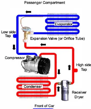
Mobile Air Conditioning system is an integrated system of components that provides cooling to vehicles. Any MAC system uses four basic parts as shown in Figure 1.1 :
Figure 1.1 Basic components of a MAC system and circuit of the refrigerant flow.
A belt-driven mechanical compressor, driven by the vehicle engine
A thermal expansion valve (TXV) for the expansion of refrigerant from the high-pressure side to the low-pressure side; when the MAC system is stopped the TXV is open
Two heat exchangers: condenser and evaporator;
Suction line, discharge line, and liquid line that connect each component to the other making a single circuit.
The belt-driven compressor uses engine power to compress and circulate the refrigerant gas throughout the system. The refrigerant passes through the condenser on its way from the compressor outlet to the TXV. The condenser is located outside the passenger compartment, in front of the vehicle radiator.
The refrigerant passes from the TXV to the evaporator, and after passing through the evaporator circuit, it is returned to the compressor inlet. The evaporator is located inside the vehicle passenger compartment.
When the compressor starts running, it pulls refrigerant from the evaporator and forces it into the condenser, thus lowering the evaporator pressure and increasing the condenser pressure. When proper operating pressures have been established, the TXV expands the refrigerant to return to the evaporator, the refrigerant mass flow rate leaving the TXV equals the refrigerant mass flow rate entering the compressor in steady state regime. Under these conditions, the pressure at each point in the system will reach a constant level; the condenser pressure will be in the range of 1.3 to 2.7 MPa depending on the outdoor temperature and the refrigerant mass flow rate; the evaporator pressure is controlled by the TXV in the range of 0.3 to 0.4 MPa. Those values of pressures are related to HFC-134a refrigerant.
The pressure in the evaporator is controlled in order to be in any case just above the water frosting temperature (0°C). In summary the evaporation of refrigerant at low temperature removes heat from the vehicle cabin and heat is transferred through the compression at a
1.2 Current Refrigerant HFC-134a Emissions
As of 1991, CFC-12 used in MAC systems has been replaced by HFC-134a, which is non-ozone-depleting refrigerant, and by 1994 almost all new vehicles sold in developed countries used this refrigerant thanks to the enforcement of the Montreal Protocol.
Table 1.1 Evolution of the CFC-12 and HFC-134a fleet [IPC05].
Figure 1.2 Mobile air conditioning fleet evolution from 1990 to 2015 in the BAU scenario [IPC05].
According to Table 1.1, the global CFC-12 fleet has decreased from about 212 million vehicles in 1990 to 119 million vehicles in 2003, while the HFC-134a fleet has increased from 1 million in 1992 up to 338 million in 2003. According to a business as usual (BAU) scenario, this value will reach 965 million by 2015 [IPC05]. Table 1.2 and Figure 1.3 present emission contributions for each refrigerant. Figure 1.3 and Figure 1.4 translate the emissions into equivalent CO2 emissions based on refrigerant GWP. Due to the huge difference of their GWPs, Figure 1.4 shows the significant decrease of refrigerants emissions from 848 Mt CO2 -eq in 1990 to 610 Mt CO2-eq in 2003. Hence, it is clear that the conversion from CFC-12 to HFC-134a has a positive effect for limiting global warming.
Table 1.2 MAC refrigerants emissions [IPC05]. Table 1.3 MAC refrigerants emissions in CO2_eq
[IPC05].
Figure 1.3 MAC refrigerant emissions from 1990 to
1.3 Classification of MAC Refrigerant Loss And Leakage
Source
According to test data, 50% to 60% of identified leaks are due to the compressor, hoses or crimps. Other leak sources are the expansion valve (TXV, or orifice tube), the receiver, the control switch, the service valve, etc. It could be said that almost all the MAC components leak.
There are six main types of leaks or emissions during the life cycle of the vehicle. Emissions have to be distinguished from leaks in this section. Leaks are coming from the clearance of mechanical part and from diffusion through elastomer materials. Emissions are linked to any operation on the MAC system where refrigerant is handled.
1. Emissions at initial charge of the MAC system
They are usually low due to the use of proper evacuation and refrigerant charging equipment. Nevertheless, the cylinder management leads to emissions varying from 1 to 10% depending on the recovery of the remaining refrigerant in the cylinder refrigerant heels. 2. Regular leak for new system
Hoses, O-rings, and the rotary shaft seal of the compressor are weak points in the sealing system constituting the essential points of regular refrigerant leakage from MAC systems. Leakage sources coming from this part will be discussed in detail.
3. Leaks due to leak tightness degradation
The aging process for leak tightness is difficult to simulate, even if some compressors tests show that the degradation seems low providing correct lubrication. Moreover, studies of vehicles older than 8 years are difficult to perform, and until now few specific data are available. Except that the refrigerant market for servicing indicates that leak degradation is the sole explanation for the use of those refrigerant quantities.
4. Irregular leakage caused by accident and component failures
Accidents are the main factors of the irregular leakage of MAC systems, such as the puncture of the condenser, exposition of hoses, damages of crimps, and road accidents.
5. Emissions during servicing
During the system servicing, leakages could occur due to the low skill, inadequate knowledge of operators, and improper use of refrigerant connecting lines from the refrigerant recovery & recharge equipment. Moreover, in some countries the use of small cans lead to significant emissions for servicing.
6. Emissions at end of life (EOL) of the system
The lack of recovery or the poor recovery efficiency of the refrigerant, when the system is disassembled at the end of lifetime, has to be taken into account.
• Compressor
The MAC compressor is belt-driven and with open shaft compressor. The shaft is linked to the engine by a pulley/belt system. The leak tightness is ensured by the rotary shaft seal, which plays an important role to guarantee the leak tightness of refrigerant gas both in running and standstill modes. Moreover, the coupling and the drive-belt pulley are two significant causes of the refrigerant leakage. In running mode, the belt presents the risk of pulling the shaft away from its centerline, which will decrease the tightness of the seal. The leak tightness depends also on appropriate lubrication of the seal.
Figure 1.5 Cross section of a compressor.
The most common compressor shaft seals are of the lip seal type. The lip seal is typically made of highly saturated rubber encased in steel. One typical lip seal used in MAC compressors is illustrated in Figure 1.6. The first lip is placed at the high-pressure side and is responsible for sealing fluid in standstill mode. The second lip, normally made of PTFE, is placed at the low-pressure side (atmospheric pressure) and is responsible for sealing fluid in running mode. Shaft compressor is then inserted in the seal and, as a result, the two lips contact the shaft surface. Experimental results show a contribution of 50% of shaft seal to total leak flow rate of a compressor [SOU08].
Figure 1.6 Details of a compressor shaft lip seal [SOU007].
Results on 24 new compressors at 40°C in standstill mode show that the leak flow rates vary from 5 to 22 g/yr leading to an average value of 14 g/yr. The shaft seal is not recovering its original leak tightness by aging and the leak flow rate of a compressor from an end of life vehicle may rise up to 180 g/yr. In running mode, leak flow rate strongly depends on the velocity of compressor and on the viscosity of lubrication oil [SOU07].
• Hoses
Flexible material hoses are used in MAC systems to connect different parts of the system because they absorb vibrations and accommodate movement of the engine. They are also a
source of significant refrigerant leak. Therefore it is important to choose low permeation hoses, which appear suitable for MAC systems.
All-rubber hose
Nylon Barrier hose
Nylon Composite (veneer) hose The hose permeation is the most important parameter to
determine the leakage of this component. Permeations of hoses are quite different depending on their material compositions and diameters. According to the results of several tests carried out during this research work (see Chapter 3), the presence of refrigerant oil has only a modest effect on permeation. That means that the leak flow rate of a hose with the charge of HFC-134a and oil is lower than the LFR of the same hose charged only of HFC-134a.
Different types of hose technologies are currently used in MAC systems.
All rubber, nylon composite (so called veneer) and nylon barrier hoses are currently used for MAC HFC-134a systems. Veneer hoses typically have a thin nylon inner liner that acts as permeation barrier. Nylon barrier hoses also use a thin nylon layer to prevent refrigerant permeation. However, they also contain a nitril or chloroprene (also known as neoprene) liner inside the nylon, which presents an excellent sealing against the coupling surface.
Figure 1.7 Three different types of MAC (by courtesy of MAFLOW).
All of liquid line, discharge line, and suction line have always elastomer sections as well as metallic ones. Commonly used internal diameters are 8, 10, 13, and 16 mm. All rubber hoses are often chosen for suction line due to their high performance in absorbing the compressor vibrations and noises.
• Crimps
Hose crimps are used to connect the flexible hose and the aluminum tube. The aluminum is exclusively chosen for its easiness of shaping and cost. An example of barrier hose is given in Figure 1.8 with the construction from inner to outer: a CR (Chloroprene Rubber) inner tube, a PA(polyamide) barrier, a layer of braid reinforcement, and an EPDM (Ethylene Propylene Diene Monomer) cover.
(1) aluminum tube (2) crimps (3) EPDM cover (4) braid reinforcement (5) PA barrier (6) CR inner tube
Figure 1.8 Cross section of crimps.
leakage. If the inner layers are soft elastomer as shown in Figure 1.9(c), glue or nothing is used instead of seals because of the good deformation of soft polymers.
(a) integral D-Ring fitting crimps
(b) Integral double O-ring fitting for crimps
(c) Glue used crimps
Figure 1.9 Different types of crimps (by courtesy of MAFLOW).
Possible leakage due to the crimps includes the damage of the crimps by accident, and progressive performance loss of the sealing technology. However, the leak flow rates of crimps are low (< 0.1 g/yr) compared to other MAC components.
• Fittings/Connectors
Connectors connect different parts of MAC systems. Assembly of connectors on the pipes or with the principal components has to guarantee a rigorous tightness to contain the pressures of the system in both standstill and running modes.
(1) Connector with simple support
(2) Connector with screwed ends
(3) Connector with spring lock (clipped on connector)
Figure 1.10 Typical connectors.
In general, connectors used for MAC systems consist of connectors with simple support, connectors with screwed ends, and connectors with spring lock (3) (see Figure 1.10).
Connectors with support (1) are the most commonly used on MAC systems. Advantages of those connectors are: easy assembly of the MAC components and simplification of the angular orientation of the pipes.
For connectors with screwed ends (2), torques applied to connectors seem to be more important to determine the emission level.
The spring lock connector (3) is the most practical for assembly but may be the most emissive due to the free rotation along the axis.
• Evaporator and Condenser
Since the mid ‘90s, condensers are made of louvered fins micro-channel tubes connected in parallel and in series. Some of them have integrated high-pressure receiver. Condensers are mounted in front of the radiator to take advantage of the forced air provided by the fan and the motion of the car. Figure 1.11 shows the principle of a multi-flow condenser and the micro-channel structure. Evaporator could be of plate-and-fin technology or, recently, of the same louvered-micro-channel technology as the condenser, but with a specific arrangement for refrigerant distribution. Figure 1.12 shows a multi-tank evaporator and the micro-channel structure. Both of them are fully brazed and leak tight, and the emission level is assumed lower than 0.1 g/yr.
Figure 1.11 Condenser and the micro-channel structure
Figure 1.12 Evaporator and the micro-channel structure
The condenser is the highest risk component in case of crashes or stone hits because it is placed in the vehicle front end. A thrown stone can destroy the surface of one of the flat tubes that will then corrode at the point of impact. At the end of a period of time, leakage will take place. When the condenser is damaged, 100% of the refrigerant is lost. According to Valéo Clim Service nearly 7000 condensers have been replaced in 2002.
• Thermal Expansion Valve (TXV)
The function of a TXV is to expand the refrigerant from the condensation pressure to the evaporation pressure to control the refrigerant flow depending on the cooling needs. "H block" type TXV (Figure 1.13) is commonly used in MAC systems. It is located between evaporator inlet and outlet tubes, the liquid line, the compressor, and sealed by O-rings at
temperature and controls the refrigerant flow rate to the evaporator. When the operating pin pushes the ball away, the connection between the inlet side of the liquid line and the outlet side to the evaporator is connected so that gas can pass through. The valve spring is used to put the ball to the initial position when the connection is closed. As shown in Figures 1.13 and 1.14, not only leakage emissions are due to four O-ring seals but also to the top-side sensing parts which are also assembled by seals.
outlet to comperssor discharge from evaporator outlet to evaporator internal equalization passage sealed sensing bulb operating pin inlet from liquid line
metering orifice
valve spring valve diaphragm
Figure 1.13 Photo of “H block” type TXV. Figure 1.14 TXV structure.
• Service valve
Figures 1.15 illustrates the cross section of the service valve with its usual location on suction line for low pressure and liquid line for high pressure in order to charge the refrigerant to the MAC system or to recover it. Generally two seals are mounted with the purpose of improving the valve leak tightness. They are respectively:
a micro lip seal inside the valve core, which protects the refrigerant from leaking by the force of the spring,
a barrel seal, which is deformed by the valve housing when fixing the valve core inside the valve body,
additionally, the cap is also a complementary prevention to the refrigerant leakage.
Detail of lip seal Detail of barrel seal
Figure 1.15 Sealing technology of service valve (by courtesy of VENTREX).
deformed barrel seal valve housing
• High pressure sensor
A MAC system is equipped with a high-pressure sensor, which senses the pressure of the refrigerant discharged from the compressor and controls the fan coupled to condenser. As shown in Figure 1.16, an O-ring seal is used to seal the part by screwing the pressure sensor on the tube.
Figure 1.16 High-pressure sensor. • Other factors
Compressors require a lubricant to protect its internal moving parts and ensure its operation. Lubrication oil (PAG Poly-alkyl-glycol) presents a better suitability with HFC-134a. Additionally, lubrication oil has a positive effect on leak flow rates of the MAC system since the fluid viscosity of lubrication oil is quite higher than that of refrigerant gas.
To conclude, the leakage phenomena are quite complex and depend on many factors: the refrigerant temperature and pressure; environment factors such as vibrations; the geometry and material of each component of the MAC system; torques applied to fittings, assembly process of the system, etc. This thesis focuses on the research of regular leak from new MAC systems and investigates emission predictions from those systems.
1.4 References
[IPC05] IPCC Special report. 2005. Safeguarding the ozone layer and the global climate system. Issues related to hydrofluorocarbons and perfluorocarbons. Cambridge University Press. ISBN 13 978-0-521-68206-0.
[SOU07] Sousa, D., Denis, C., 2007. Measurement of mobile AC compressor fugitive emissions in running mode. 6th EDF/LMS workshop: Role and effect of contact surfaces in dynamic sealing. Poitiers, France, 2007.
[SOU08] Sousa, D., Denis, C., 2007. Sealing performance of a Mobile AC compressor shaft seal. 2008 International compressor engineering and refrigeration and air conditioning conferences. Purdue, USA, July 14-17, 2008
CHAPTER 2 Leak flow rate method
CHAPTER 2
Leak flow rate method
List of Figures
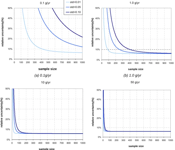
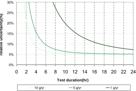
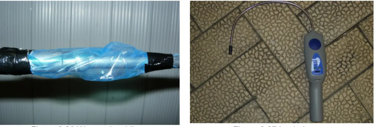
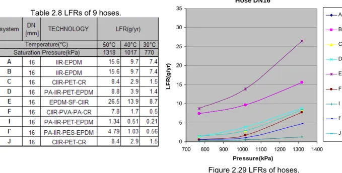
Figure 2.1 Scheme of the measurement system... 19 Figure 2.2 IR spectrophotometry Uras-14 measurement principle (by courtesy of ABB). ... 21 Figure 2.3 Simplified layout of the IR photo-acoustic (PAS). ... 22 Figure 2.4 PAS Innova-1314 Measurement principle (by courtesy of Innova)... 22 Figure 2.5 Flowchart of test protocol. ... 25 Figure 2.6 Standardized gas of HFC-134a/N2... 25 Figure 2.7 HFC-134a calibrated leak. ... 25 Figure 2.8 Volume calibration data... 26 Figure 2.9 Temperature and pressure variation vs. time. ... 28 Figure 2.10 Tolerance band as a function of temperature. ... 29 Figure 2.11 Concentration measurement and LFR... 31 Figure 2.12 Uncertainty contributions on leak flow rate measurement. ... 32 Figure 2.13 Measurement uncertainties as a function of the sample size. ... 33 Figure 2.14 Relative uncertainty of LFR vs. test duration (system test bench)... 34 Figure 2.15 Relative uncertainty of LFR vs. test duration (component test bench). ... 34 Figure 2.16 Test bench for system measurements... 35 Figure 2.17 System test mini-shed for running mode tests... 36 Figure 2.18 Layout of the component measurement test bench... 37 Figure 2.19 Layout of component measurement test bench... 37 Figure 2.20 Test bench for component leakage measurement... 38 Figure 2.21 MAC system installed on a duckboard for LFR test... 39 Figure 2.22 Concentration measurements during preconditioning. ... 39 Figure 2.23 LFRs of 10 MAC systems vs. pressure... 39 Figure 2.24 MAC system cut into parts making macro-components. ... 40 Figure 2.25 Welded end and connecting tube going through the wall of the cell... 40 Figure 2.26 Wrapped welding. ... 40 Figure 2.27 Leak detector... 40 Figure 2.28 LFR contribution of components for system b. ... 41 Figure 2.29 LFRs of crimps. ... 42 Figure 2.30 LFRs of TXV... 42 Figure 2.31 LFRs of compressor... 43 Figure 2.32 Regression curves for systems and sum of macro-components. ... 44 Figure 2.33 Daily average temperature of Seville. ... 45 Figure 2.34 Test by simulating real climatic conditions... 45 Figure 2.35 LFR of MAC system and regression curve ... 46 Figure 2.36 Test results in running mode for system V1 and system V2... 47 Figure 2.37 Refrigerant Recovery equipment. ... 49 Figure 2.38 Refrigerant loss during 9 months. ... 50 Figure 2.39 Results of fleet tests... 51 Figure 2.40 Establishing the correlation factor... 52
List of Tables
Table 2.1 Accuracies of different apparatuses... 20 Table 2.2 Comparison between and IR spectrophotometer and IR PAS... 23 Table 2.3 Statistical analysis of the slope. ... 31 Table 2.4 Uncertainty budget for a given example... 32 Table 2.5 Required sample size and measurement duration for 1 g/yr. ... 33 Table 2.6 LFRs of 10 MAC systems... 39 Table 2.7 LFRs of components of MAC system b... 41 Table 2.8 LFRs of 6 crimps. ... 42 Table 2.9 LFRs of 10 TXV... 42 Table 2.10 LFRs of 10 compressors ... 43 Table 2.11 LFRs and linear regression. ... 43 Table 2.12 LFRs of MAC system X at 3 different temperatures... 46 Table 2.13 Annual LFR for systems V1, V2, and V3... 47 Table 2.14 LFRs contribution in standstill and in running mode. ... 48 Table 2.15 Results of charge and recovery operation. ... 50 Table 2.16. Annual loss of Refrigerant – Vehicles A... 50 Table 2.17 Average annual losses for 10 types of vehicles. ... 51 Table 2.18 Arithmetical average LFRs of system A-J. ... 51 Table 2.19 Annual LFR predictions of 3 MAC systems based on the method of correlation factor... 52
2.1 Leak flow rate measurements
2.1.1 Test method based on measurement of concentration in an
accumulation volume
The method used to determine the leak flow rate (LFR) [CLO04b],[CLO96] is based on Equation (2.1).
t
n
M
m
HFC a HFC a HFC a∂
∂
⋅
=
− − −134 134 134&
(2.1) Where,C
T
R
V
P
C
n
n
amb accum amb total a HFC⋅
⋅
⋅
=
⋅
=
−134 (2.2)The mass flow rate is the product of molar mass and the derivative of the number of moles of HFC-134a along the time in a tight volume, the test chamber. The perfect gas law is used to take into account the small variations of pressure and temperature inside the test chamber. According to Equation (2.2), the following parameters need to be determined for leak flow rate calculation: the accumulation volume of the test chamber, the temperature and the pressure inside the test chamber, and the evolution of concentration along the time.
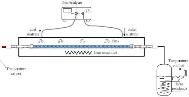
As shown in Figure 2.1, the test bench is composed of an accumulation volume at atmospheric pressure (Figure 2.1) where the component to be analyzed is installed and connected to a HFC-134a boiler generating a given level of pressure inside the component. For system measurement, the operation becomes simpler because the refrigerant is directly charged in the MAC system. The temperature of the component is controlled by heat resistance and fans, in order to be maintained always above the saturated temperature of HFC-134a at the test pressure. concentration measurement accumulation volume component HFC-134a boiler system concentration measurement accumulation volume component HFC-134a boiler system
Figure 2.1 Scheme of the measurement system.
The concentration analyzer is connected to the accumulation volume by a closed circuit and measures continuously the accumulated concentration of HFC-134a inside the volume. Knowing:
the volume of the accumulation volume, the time,
the concentration at each time step, and
2.1.1.1 Concentration
measurement methods
In order to measure leak flow rates in the range of 10-8 to 10-4 mole/s, four different types of apparatuses can be possibly used to measure the refrigerant concentration inside control volumes. Those apparatuses are based on different physical principles:
mass spectrometry, gas chromatography, infrared spectrophotometer,
Infrared photo-acoustic spectroscopy.
Accuracies of the different techniques are indicated in Table 1.1.
Table 2.1 Accuracies of different apparatuses.
Apparatuses Mass spectrometer Gas chromatography Infrared photo-acoustic spectroscopy Infrared spectro photometry Accuracy
±
1 ppb±
1 ppb±
0.01 ppm±
0.5 ppm Mass spectrometryMass spectrometry allows the mass measurement of molecules. The five basic parts of any mass spectrometer are:
a vacuum system,
a sample introduction device, an ionization source,
a mass analyzer, and an ion detector.
A mass spectrometer determines the molecular weight of chemical compounds by ionizing, separating, and measuring molecular ions according to their mass-to-charge ratio (m/z). The ions are generated in the ionization source by inducing either the loss or the gain of a charge (e.g. electron ejection, protonation, or deprotonation). Once the ions are formed in the gas phase they can be electrostatically directed into a mass analyzer, separated according to mass, and finally detected. The result of ionization, ion separation, and detection is a mass spectrum that provides molecular weight or even structural information.
Gas chromatography
Gas chromatography is widely used in all chemical and processes laboratories. It is a reference method used to measure atmospheric concentration of a tracer gas. The accuracy is one of the best of all the methods (± 1 ppb).
The only difficulty associated to gas chromatography is related to the sampling method, which implies uncertainties on the concentration of the sample compared to the concentration in the control volume. Also a significant delay could occur between the sampling and the analysis depending on the design of the measurement system. However, this method can be used for MAC systems.
Infrared spectrophotometer
The principle of the non-dispersive infrared spectrophotometry method uses characteristics of individual gases when absorbing specific infrared wavelength when infrared light is radiated to the sample gas. The monitor measures the composition and concentration by
analysis of the absorbed wavelengths. The method that uses the infrared rays of all wavelengths radiated from the light source is referred to as "non-dispersive."
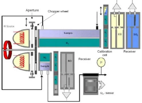
Figure 2.2 IR spectrophotometry Uras-14 measurement principle (by courtesy of ABB).
Figure 2.2 presents the measurement principle of IR spectrophotometry Uras–14. The photometer consists of an infrared source, the emissions of which reach a sample cell via a chopper wheel. The sample cell is in the shape of a tube divided by a wall into sample and reference sides. Two equal-energy infrared beams are directed through these two sides. The measurement effect produced in the receiver is a pressure effect resulting from the chopper frequency, received by a diaphragm capacitor and converted into an electrical signal by a pre-amplifier. The quantity of absorbed infrared radiation is proportional to the absorbing gas concentration. The receiver is a two-layer device. The back of the receiver has an optically transparent window so that any residual radiation can reach a second receiver that is sensitive to a second sample component. By adding a second beam path with an emitter, sample cell, and receivers, the photometer can measure 1 to 4 sample components at the same time.
Concerning the calibration, zero point calibration can be carried out with inert gas (N2)t. The end point calibration necessitates gas-filled calibration cells or test gas mixture.
Infrared photo-acoustic spectroscopy(IR PAS)
The photo-acoustic effect is based on the conversion of light energy into sound energy, and a sound-measuring device detects the signal.
The gas to be measured is irradiated by modulated light of a pre-selected wavelength. Radiation absorbed by the molecule from a modulated infrared light beam is efficiently converted into heat energy of the gas molecules, and therefore a temperature and pressure increase in the gas. The pressure will result in an acoustic wave, which can be detected by a sound-measuring device, such as a microphone. The sound pressure,
P
sound, can be calculated using the Equation 2.3.c o v p sound f I C C C K P ⋅ ⋅ − = ) 1 ( (2.3)
Figure 2.3 Simplified layout of the IR photo-acoustic (PAS).
where,
K
is a cell and gas dependent constantp
C
andC
vare heat capacities at constant pressure and volumeC is the gas concentration
c
f
is the modulation frequencyo
I
is incident lightFigure 2.4 PAS Innova-1314 Measurement principle (by courtesy of Innova).
The IR PAS system presented here, named Innova-1314, is optimized for the quantitative detection of the gas concentration. As illustrated in Figure 2.4, the instrument uses a heated nickel-chrome wire as its infrared radiation source. The light from the source is focused by an ellipsoidal mirror, modulated with a mechanical chopper, which pulsates it, and passes through one of the optical filters in the wheel before entering the photo-acoustic gas cell. The filter allows irradiating the specific gas with the exact wavelength it absorbs best.
The pomp draws a sample from the sampling point through the air-filter to flush out the “old” sample in the measurement system and replace it with a new sample. The “new” sample is hermetically sealed in the analysis cell by closing the inlet and outlet valves. The IR radiation is absorbed by the gas and generates heat and pressure variations in the closed cell. A pair of microphones mounted in the cell walls measures this acoustic signal. By selecting an appropriate resonant mode of opposite phase, the difference signal of the two microphones results in a doubling of the signal amplitude and noise reduction. The electrical signals from the microphones are amplified and added together before being sent to an analogue-to-digital converter. The analogue-to-digital signal is then converted to the concentration of the monitored gas sample present in the cell. The filter wheel turns so that light is transmitted through the next optical filter, and the new signal is measured.
The first calibration of the monitor is done just after the installation of the optical filters. Recalibration is accomplished by introducing the standardized concentration.
Comparison between the IR spectrophotometer (Uras-14) and PAS (Innova-1314)
Gas chromatography, IR spectrophotometer, and IR PAS are the three methods that could possibly be used at atmospheric pressure. Moreover, IR spectrophotometer and IR PAS are two powerful techniques commonly used to measure small absorptions and can be applied to detect trace gases in ambient air at atmospheric pressure. Both gas monitoring systems are available at the Center for Energy and Processes of Ecole des Mines in Paris and present a high accuracy, reliability, and stability. Table 2.2 makes some comparisons of IR spectrophotometer (Uras-14) and IR PAS (Innova –1314) specifications.
Table 2.2 Comparison between and IR spectrophotometer and IR PAS.
Concentration measurement Specification IR spectrophotometer
(Uras-14)
IR PAS
(Innova –1314)
Gas sample Gas sample at atmospheric pressure
Calibration
Zero and end point calibration with gas mixture & automatic calibration by means of internal calibration cell
Zero and end point calibration with gas mixture
Cross-compensation Capable Measurement cell
volume Around 40 cm
3 3 cm3
Measurement cell status Open Closed
Operation mode Continuous scan Step scan and nearly
continuous scan
Stability
≤
1% of measured value perweek
Change in sensitivity at 25°C: <10%/600 yrs
Detection limit 0.5 ppm 10 ppb
Measuring range Two ranges:
0-50 ppm, 0-500 ppm 100 000 times of detection limit
According to the measurement principle of monitors, both are suitable for concentration measurement of gas in ambient air at atmospheric pressure and can measure as many samples as necessary.
Calibration can be done at least at zero and end point. Additionally, Uras-14 is equipped with an internal calibration cell for automatic calibration. As many gases absorb well in the IR area, it is often necessary to compensate for interfering components. For instance, CO2 and H2O often initiates cross sensitivity in the infrared spectrum. Uras-14 and Innova-1314 take this interference problem into consideration. All the cross-compensation factors are calibrated and stored in the monitor during the calibration.
Uras-14 is especially suitable for the continuous-scan mode. Innova-1314 is capable of operating in both step scan and nearly continuous modes, which means that each step of scan is performed one after the other. When measuring several samples of components simultaneously, Innova-1314 can be easily used to measure the concentration alternatively. Due to the high power pomp of Uras-14, measurement is not limited by the distance between the accumulation volume and the analyzer, which is not the case for Innova-1314.
Concerning the stability, instruments based on PAS are quite stable because of the use of one of the most stable transducers: microphones. The two microphones enable to minimize interference from vibration.
The volume of the measurement cell Innova-1314 (3 cm3) is smaller than that of the Uras-14 (40 cm3). Because of its volume, the Innova cell can be emptied quickly; the samples of gases are small and so the response time is short.
Concerning HFC-134a measurements, the detection limit is 0.5 ppm for Uras-14 and 10 ppb for PAS Innova-1314, so that PAS Innova-1314 offers a higher sensitivity for concentration detection. However, because of the limit of resolution (1%) of PAS Innova-1314, it is better to perform low concentration measurement with Innova-1314. For long test period with rapid increase of concentration, Uras-14 is more convenient.
More extended comparison has been made [MOR07] not only theoretically but also experimentally by I. Morgado for the development of leak standard [MOR08]. Based on the operating principle, the photo-acoustic detection is more direct than the spectrophotometer. Microphones used in the PAS to detect the acoustic pressure generated by gas are extremely linear in a wide range of sound pressure. Their detection limits are defined as twice the detection limit of the pressure sensor, which is about the μPa. For HFC-134a, a sound pressure around the µPa corresponds to a concentration detection limit around 15 nmol.mol-1. However, for the spectrophotometer, the pressure sensor is not linear. The signal is converted numerically and linearized. In terms of measuring environment, thus, the spectrophotometer seems to be more efficient to attenuate the noise signal. A series of experimental data show that the repeatability and linearity are about 10 times better than that of the spectrophotometer, at low concentrations.
2.1.1.2 Testing
protocol
The test protocol for leak flow rate measurements is described step by step in Figure 2.5.
Step 1: Standardization of the concentration measurement apparatus
The first step is to verify the concentration measurement apparatus. As shown in Figure 2.5, a standardized concentration of HFC-134a in nitrogen (delivered by accredited companies) is connected to the measurement apparatus, and the measured value is compared to the standardized concentration. This verification is repeated with a second higher concentration. These two measurements verify both the offset and the linearity of the measurements of concentration by the apparatus.
Standardization of the concentration measurement apparatus
Standardization of the concentration measurement apparatus Calibration of the accumulation volume Calibration of the accumulation volume Calibration of temperature and pressure Calibration of temperature and pressure Test procedure Steady state conditions Temperature and pressure control
Test procedure Steady state conditions Temperature and pressure control
Calculation of leak flow rate uncertainty analysis
Calculation of leak flow rate uncertainty analysis
Figure 2.5 Flowchart of test protocol.
Step 2-1: Calibration of the test chamber
The uncertainty of the LFR is directly related to the uncertainties on the free volume of the test chamber. First the volume is calculated based on the geometric descriptions. Then a standard calibrated leak (see Figure 2.7), which has been calibrated on a specific test chamber, is installed inside the test chamber to be calibrated.
Figure 2.8 gives an example of calibration of the accumulation volume. The calibrated leak is measured at constant temperature of 26°C. As indicated in the figure, all parameters such as temperature, pressure, and concentration inside the test chamber are recorded at each time step. The leak flow rate of calibrated leak at 26°C is known as 51.1 g/yr. The accumulation volume can be obtained by reverse calculation of the mass flow rate, which is expressed by Equation (2.4) and consequently its uncertainty is established, which will be discussed in the following section. Figure 2.6 Standardized gas of HFC-134a/N2. Figure 2.7 HFC-134a calibrated leak.
t
C
RT
P
M
m
V
amb a HFC a HFC accum∂
∂
=
− − 134 134&
(2.4)Step 2-2: Calibration of temperature and pressure sensors
As shown in Equation (2.2), both temperature and pressure values inside the test chamber contribute to the LFR value. Before installation in the test bench, temperature and pressure sensors are carefully calibrated. The accuracy of both sensors is established through their calibration, which will be discussed later.
Volume accumulation calibration Calibrated leak@26°C LFR: 51.1 g/yr 0 5 10 15 20 25 30 35 40 45 50 55 60 0 1 2 3 4 5 6 7 8 9 10 11 12 13 14 15 16 Time (hr) LF R(g /yr) & Te mp er at ur e( °C) 0 1 2 3 4 5 6 7 8 9 10 Co nc en tr at io n( pp m) & P re ss ure (b ar ) LFR(g/yr) Temperature HFC-134a concentration Pressure
Figure 2.8 Volume calibration data.
Step 3: Testing procedure
After installation of the test sample, the test chamber is closed and then rinsed by a reference gas (reconstructed air: 80% N2 + 20% O2) in order to exclude all possible suspicious particles and guarantee the accuracy of measurement. The pressure is kept at atmospheric pressure. The temperature is maintained constant as well as during the test period. At each time interval, concentration, temperature, and pressure are recorded by the data acquisition system.
Tests can be performed either at a single temperature and pressure or at several temperatures and pressures. It is better to use at least three measurement points in order to verify the LFR variations according to saturating pressures.
Step 4: Calculation of leak flow rate
Based on Equations (2.1) and (2.2), the leak flow rate is calculated and the measurement uncertainty is established. Estimation on the uncertainty of leak flow rate test plays an important role, which indicates the reliability of a measurement, so that we will focus on the uncertainty analysis.
Other considerations
Repeatability
Repeatability is the property verified by using exactly identical procedures, identical testing systems, identical operators, and identical measurement apparatuses for identical components and to verify that identical results are obtained.
Reproducibility
Reproducibility is the property that verifies different variations either in the measurement operation or in the components to be tested. Reproducibility conditions mean independent test results are obtained with the same method on identical test items in different laboratories by different operators using different equipment.
Sample size
Accuracy of measurement has to be seen in the light of statistic measurements and not based on a too limited number of samples. When measuring the concentration in a control volume, when the raise of concentration is constant, the LFR is in steady state. Three to four points are the minimum sampling numbers. Some apparatuses can make hundreds of samplings within a measurement period from 10 to 12 hours, and so the statistical accuracy is significantly improved (see § 2.1.1.3).
2.1.1.3 Uncertainty
analysis of LFR measurement
Based on the principle of indirect measurements from the propagation of distributions, the uncertainty of leak flow rate is achievable [GUI93]. Since the temperature and pressure are maintained constant during the test, the leak flow rate of the component under test can be calculated according to Equations (2.1) and (2.2). All these uncertainty sources and their influences will be analyzed based on the experimental data (presented in Figure 2.10 and Figure 2.11).
Identification of each uncertainty source
Two contributors to measurement uncertainties are distinguished here.
• Type A: this type of uncertainty can be determined statistically by measuring the
dispersion of values obtained from well-chosen standard deviation of samples. In other words, the uncertainty of type A is quantified by calculating the standard deviation from repeated measurements.
• Type B: this type of uncertainty must be determined by non-statistical methods. Type B
contributor will be the uncertainty of the reference standards and reference materials, which can never be picked up statistically.
The functional relationship between the leak flow rate
(
m
&
)
and the input quantities(
t
C
V
P
T
amb amb accum∂
∂
,
,
,
) is given by Equation (2.5).)
,
,
,
(
)
(
t
C
V
P
T
f
x
f
m
i amb amb accum∂
∂
=
=
The total uncertainty of the leak flow rate is a combination of 4 uncertainty components. By applying the law of propagation, the combined standard uncertainty of the mass flow is written in Equation (2.6): ) / ( / ) ( ( ) ( ) ( 2 2 2 2 ) 2 2 2 t C u t C m P u P m T u T m V u V m m u amb amb amb amb accum accuù ∂ ∂ ⎟ ⎠ ⎞ ⎜ ⎝ ⎛ ∂ ∂ ∂ + ⎟⎟ ⎠ ⎞ ⎜⎜ ⎝ ⎛ ∂ ∂ + ⎟⎟ ⎠ ⎞ ⎜⎜ ⎝ ⎛ ∂ ∂ + ⎟⎟ ⎠ ⎞ ⎜⎜ ⎝ ⎛ ∂ ∂
= & & & & (2.6)
Therefore, the standard relative uncertainty is calculated according to Equation (2.7).
2 / 2 2 2 134
/
⎟
⎠
⎞
⎜
⎝
⎛
∂
∂
+
⎟⎟
⎠
⎞
⎜⎜
⎝
⎛
+
⎟⎟
⎠
⎞
⎜⎜
⎝
⎛
+
⎟⎟
⎠
⎞
⎜⎜
⎝
⎛
=
∂ ∂ −C
t
u
P
u
T
u
V
u
m
u
t C amb P amb Tamb accum V a HFC m accum amb&
& (2.7)Each uncertainty source is analyzed in detail as follows.
Figure 2.9 Temperature and pressure variation vs. time.
(1) Temperature inside the test chamber
According to manufacturer’s specifications, the tolerance for a temperature sensor Pt100 of class A is written as: ΔT =0.15+0.002×T , where T is the measured temperature in °C.
Figure 2.10 shows the tolerance with regards of measured temperature. The uniform distribution is applied to obtain Type B uncertainty estimate. Knowing the limits of temperature values, the uncertainty is estimated by Equation (2.8) using the assumption of a rectangular distribution for the temperature variation.
3
) (T
u
T typeBΔ
=
(2.8)The standard uncertainty of Ttype A means the repeatability standard deviationsT, which can be obtained by statistic analysis of n observations of temperature. As shown in Figure 2.9, a series of temperature values are recorded during the test.
1 ) ( 1 2 ) ( − − = =
∑
= n T T s u n i i T typeA T(2.9)
-0,6 -0,5 -0,4 -0,3 -0,2 -0,1 0,0 0,1 0,2 0,3 0,4 0,5 0,6 -50 -40 -30 -20 -10 0 10 20 30 40 50 60 70 80 90 100 Temperature (°C) T o ler an ce (° C )Figure 2.10 Tolerance band as a function of temperature.
Therefore, the uncertainty of the temperature uT can be determined by combining the uncertainties of Type A and Type B using the technique of root mean square sum:
2 1 2 2 ) ( 2 ) ( 3 1 ) ( ⎟⎟ ⎠ ⎞ ⎜⎜ ⎝ ⎛ Δ + − − = + =
∑
= T n T T u u u n i i typeB T typeA T T (2.10)Based on the temperature data shown in Figure 2.9, a mean value of 40.64°C and a standard deviation of 0.035°C are obtained.
C T s u u uT T typeA T typeB T ⎟⎟ = ° ⎠ ⎞ ⎜⎜ ⎝ ⎛ + + = ⎟⎟ ⎠ ⎞ ⎜⎜ ⎝ ⎛ Δ + = + = 0.14 3 64 . 40 * 002 . 0 15 . 0 035 . 0 3 2 2 2 2 2 ) ( 2 ) ( (2.11)
Relative standard uncertainty is obtained by dividing the uncertainty by the mean temperature value: 4 10 5 . 4 64 . 40 15 . 273 14 . 0 = × − + = T uT (2.12)
(2) Pressure inside the test chamber
Depending on the same principle, the uncertainty of the ambient pressure value is measured by using a pressure sensor of 0-200 kPa abs, which has an accuracy of 0.2% of full scale. The estimated uncertainty of type B can be calculated:
3 400 3 10 2 % 2 . 0 5 ) ( Pa Pa uPtypeB = × ⋅ = (2.13)
The Type A uncertainty is obtained based on the data given by Figure 2.10. The uncertainty coming from the pressure is expressed by Equation (2.14).
2 1 2 2 ) ( 2 ) (
3
400
1
)
(
⎟⎟
⎠
⎞
⎜⎜
⎝
⎛
+
−
−
=
+
=
∑
=n
P
P
u
u
u
n i i typeB P typeA P P (2.14)From the pressure data shown in Figure 2.9, a mean value of 99731 Pa and a standard deviation of 368 Pa are obtained.
Pa
s
u
u
u
P PtypeA PtypeB P368
3
400
287
3
400
2 2 2 2 2 ) ( 2 ) (⎟⎟
=
⎠
⎞
⎜⎜
⎝
⎛
+
=
⎟⎟
⎠
⎞
⎜⎜
⎝
⎛
+
=
+
=
(2.15)The relative pressure uncertainty is:
3 10 7 . 3 99731 368 = × − = P uP (2.16)
(3) The accumulation volume
The accumulation volume consists of two parts: the free volume of the test chamber before installation of a MAC system or a component and the volume of the system/component, calculated by Equation (2.17).
component FreeVolume
accum
V
V
V
=
−
(2.17)The free volume of the test chamber is determined using a calibrated leak (Figure 2.7). The calibrated leak has been installed inside the test chamber and measured at constant temperature of 26°C, at which temperature the leak flow rate is already known (51.1 g/yr). The obtained leak flow rate value helps to calculate the free volume. This calibration step leads to an uncertainty of about 6%. Moreover, the volume of the system/component can only be obtained by geometrical measurement of all components, some of which include many complex parts. As a result, its uncertainty rises up to 20%. Nevertheless, the uncertainty of this part is negligible compared to the huge free volume inside the test chamber. As demonstrated in Equation (2.18), the relative combined standard uncertainty of the accumulation volume is 6%.
06
.
0
2 2=
+
=
accum V V accum VV
u
u
V
u
accum FreeVolume component (2.18)(4) Concentration vs. time
t
C
∂
∂
As illustrated in Figure 2.11, the concentration evolution according to time is recorded at each time interval. By definition,
C
iis a linear function oft
i: Cˆi =aˆ+bˆti, where b =t
C
∂
∂
is the slope of the line. As shown in Figure 2.11, a set of data values
(
t
i,
C
i)
is observed bycontinuous measurement. The basic technique for determining the term
t
C
∂
∂
is the method of least squares, which ensures that the value fits the sample data best, in the sense of minimizing the sum of squared residuals.
The standard error of the regression is written as:
(
)
2 ˆ 2 − − =∑
n C C sregression i i (2.19)where,
n is the number of samples
(
)
∑
−
ˆ
2i
i
C
C
is the sum of squared residuals.Without taking into account errors in t, the standard error of the slope (
t
C
∂
∂
), which should not to be confused with the standard error of the regression (
s
regression), is calculated as follows:(
)
∑
−
=
2 2t
t
s
s
i regression DC (2.20) where, it
is the time of the measurementt is the mean of all
t
iEquation (2.20) shows that a high degree of variation of
t
i makes for a small standard deviations
∂ /C ∂t. The results of linear regression analysis are indicated in Table 2.3.Table 2.3 Statistical analysis of the slope.
Variable Value(ppms-1) Standard deviation(ppms-1)
t
C
∂
∂
410
3
.
1
×
−2
.
3
×
10
−8 0 5 10 15 20 25 30 35 40 45 50 0 1 2 3 4 5 6 7 8 9 10 11 12 13 14 15 16 Time (hr) LFR (g /y r) 0 1 2 3 4 5 6 7 8 9 10 C onc ent ra ti on( ppm )LFR(g/yr) HFC-134a concentration
Figure 2.11 Concentration measurement and LFR.
Calculation of the combined standard uncertainty
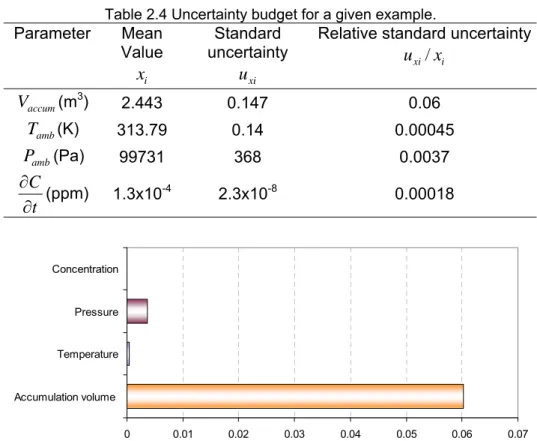
Table 2.4 summarizes the mean and relative standard uncertainties of all input values that lead to a leak flow rate of 39.5 g/yr with a relative uncertainty of 6%.
![Figure 1.6 Details of a compressor shaft lip seal [SOU007].](https://thumb-eu.123doks.com/thumbv2/123doknet/11340931.284111/19.892.163.731.685.936/figure-details-compressor-shaft-lip-seal-sou.webp)