HAL Id: hal-00941494
https://hal.archives-ouvertes.fr/hal-00941494
Submitted on 13 Nov 2020
HAL is a multi-disciplinary open access
archive for the deposit and dissemination of
sci-entific research documents, whether they are
pub-lished or not. The documents may come from
teaching and research institutions in France or
abroad, or from public or private research centers.
L’archive ouverte pluridisciplinaire HAL, est
destinée au dépôt et à la diffusion de documents
scientifiques de niveau recherche, publiés ou non,
émanant des établissements d’enseignement et de
recherche français ou étrangers, des laboratoires
publics ou privés.
analysis
Romain Monchaux, Mickaël Bourgoin, Alain H. Cartellier
To cite this version:
Romain Monchaux, Mickaël Bourgoin, Alain H. Cartellier. Preferential concentration of heavy
par-ticles : a Voronoï analysis. Physics of Fluids, American Institute of Physics, 2010, 22, pp.103304.
�10.1063/1.3489987�. �hal-00941494�
Preferential concentration of heavy particles: A Voronoï analysis
R. Monchaux,1M. Bourgoin,2and A. Cartellier21
Unité de mécanique, Ecole Nationale Supérieure de Techniques Avancées, ParisTech, Chemin de la Hunière, 91761 Palaiseau Cedex, France
2
Laboratoire des Ecoulements Géophysiques et Industriels, CNRS/UJF/G-INP UMR5519, BP53, 38041 Grenoble, France
共Received 21 April 2010; accepted 3 August 2010; published online 14 October 2010兲
We present an experimental characterization of preferential concentration and clustering of inertial particles in a turbulent flow obtained from Voronoï diagram analysis. Several results formerly obtained from various data processing techniques are successfully recovered and further analyzed with Voronoï tesselations as the main single tool. We introduce a simple and nonambiguous way to identify particle clusters. We emphasize the maximum preferential concentration for particles with Stokes numbers around unity and the self-similar nature of clustering and we report new unpredicted results concerning clusters inner concentration dependence on Stokes number and global seeding density. Some of these experimental observations can be consistently interpreted in the context of the so-called sweep-stick mechanism. Finally, we stress the great potential of Voronoï analysis that offers important openings for new investigations of particle laden flows in terms, for instance, of simultaneous Lagrangian statistics of particle dynamics and local concentration field. © 2010
American Institute of Physics. 关doi:10.1063/1.3489987兴
I. INTRODUCTION
The study of inertial particles laden flows is relevant to many industrial and environmental issues共chemical reactors and engine optimization, plankton or pollutant dispersion, clouds formation, etc.兲, but it is also of fundamental interest. A striking feature is the trend to preferential concentration that has been observed for long1,2 and which is still thor-oughly studied.3–6Another interesting feature is the enhance-ment of the settling velocity of particles in turbulent flows. Since an explanation of seeding density dependence of this phenomenon through collective effects has been proposed,7 different authors have tried to quantify and characterize par-ticles clustering from numerical simulations. Nevertheless an appropriate equation of motion for an accurate modeling of particle dynamics is still lacking, only the point particle limit is generally considered8,9and even further simplifications are usually required to achieve numerical simulations.10,11 Ex-perimental investigations are still important to reach a better understanding of the underlying mechanisms. Several recent studies have focused on the single particle problem by mea-suring the Lagrangian acceleration in order to get insight on the relevant forces acting on isolated particles.12–15 We con-sider here the many particles case to address preferential concentration and clustering matters including possible col-lective effects. Do clusters exist as a whole in these flows? How do they form? What is their structure and how does this structure evolve with time? Which effect do they have on the single particle dynamics? Here are some of the questions that still need to be answered. To date, the preferential concentration/clustering problem has been studied with glo-bal or Eulerian tools 共such as box counting methods, pair correlation function estimation, correlation dimension, or to-pological indicators兲. A dynamical study of the Lagrangian dynamics of particles and of the local concentration field
would bring a new insight in these processes. In particular, it would be worthwhile to get access to the concentration along a particle trajectory, a quantity that has been recognized as very important in models.16,17
In that scope, we propose in this article a new approach to analyze particle concentration fields based on Voronoï tes-selations that gives a measure of the local concentration field at interparticle length scale. By itself, this data processing technique is particularly enlightening to explore and quantify the preferential concentration phenomenon while, combined to Lagrangian tracking, it also gives access to simultaneous measurements of velocity, acceleration, and local concentra-tion along particles trajectories that are crucial for a better insight of clusters and particle dynamics. As a first step, this article focuses on the preferential concentration problem on a statistical ground. Section II is dedicated to the description of our experimental setup and of the tools used to postprocess the acquired data. In Sec. III, we use Voronoï analysis to quantify the preferential concentration and to identify and characterize clusters. Conclusions and expected further dy-namical studies are summarized in Sec. IV.
II. EXPERIMENTAL SETUP AND POSTPROCESSING A. Two-phase flow generation and characterization
Experiments are conducted in a large wind tunnel with a square cross-section of 0.75 m⫻0.75 m where an almost ideal isotropic turbulence is generated behind a grid whose mesh size is 7.5 cm共Fig.1兲. We can adjust the mean velocity
from 3 to 15 m s−1 共the turbulence level remains relatively
low of the order of 3% at the measurement location and the anisotropy level between the transverse and longitudinal fluctuating velocities is smaller than 10%兲. Inertial particles are water droplets generated by four injectors placed in the
PHYSICS OF FLUIDS 22, 103304共2010兲
convergent part of the wind tunnel, one meter upstream the grid to ensure a homogeneous seeding of the flow. These injectors consist of two tubes carrying water and air that merge into a specifically designed nozzle关a Schlick-Dusen 共Germany兲 942 two fluid nozzle兴 where pressurized air atom-izes the liquid and forms the exiting conic jet. The particle properties relevant to our study can be adjusted within acces-sible range. Volume loading is directly linked to the water flow rate in the nozzles while the diameter distribution is a subtle function of both water flow rate and air pressure in the nozzles, as detailed below. We always consider regimes of relatively low particles volume loading共volume fraction in our experiments covers the range 2⫻10−6⬍
v⬍3⫻10−5兲
so that no significant turbulence modulation by two-way coupling is expected to occur.
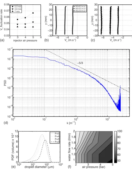
We have performed particle image velocimetry 共PIV兲 and hot-wire measurements in the test section in order to characterize the turbulence underlying our experiment. Hot-wire acquisitions have been done for the single phase air flow. They show a slowly decaying nearly homogeneous tur-bulence. When the mean flow velocity is changed from 3 to 7.5 m s−1, the associated Taylor microscale Reynolds
num-ber R varies from 72 to 114 at the measurement location situated 3 m downstream the grid. The evolution of the tur-bulence characteristics of the single phase flow at different locations downstream the grid for the explored range of mean velocities is given in Table I. In order to probe the maximum influence on the carrier turbulence of the addi-tional perturbation from the injectors, we have also measured the turbulence fluctuation level when the injectors blow only air共hot-wire measurements are not possible in the two-phase configuration兲. It is found to increase typically by 50%
com-pared to the case without injectors. Nevertheless, this en-hancement of turbulence intensity does not depend much on the imposed air pressure at the injectors as shown on Fig.
2共a兲共except at very low wind speed兲. It should also be noted
that this influence is expected to be reduced when the water flow is turned on since atomized droplets will carry a signifi-cant amount of the global additional momentum injected by the nozzle’s air flow. PIV was carried out from high speed imaging 关we use a Phantom V12 camera from Vision Re-search, Inc.共New Jersey, USA兲兴 of the injected water droplet fog. We note that although such inertial particles are not expected to follow the flow, these PIV measurements give a good characterization of the global flow homogeneity and isotropy. Figure 2共b兲 presents PIV vertical profiles of the axial velocities averaged over x along the whole measure-ment volume showing the good homogeneity of the flow in the cross-section of the tunnel; moreover, the very slow evo-lution of these profiles with the axial coordinate x along the measurement volume关Fig.2共c兲兴 evidences the slow decay of turbulence within this volume. On Fig.2共d兲, a typical veloc-ity spectrum allows to identify a narrow inertial range as expected at this moderate Rvalue.
Regarding the droplet spray, one of the main goals of our study is to explore the influence of particle diameters d共or equivalently of their Stokes number, defined as St⬅p/
=共d/兲2共1+2⌫兲/36, where p is the particle viscous
relax-ation time, and are, respectively, the dissipation time scale and length scale of the carrier flow, and⌫=water/airis
the ratio of particles density to carrier fluid density兲 on the preferential concentration phenomenon. The two-phase nozzles that we use to produce the spray present the advan-tage to easily allow a systematic variation of the mean diam-eter of droplets by controlling air and water flow rates in the injectors. The drawback of this versatility is the difficulty to produce a monodisperse spray. The injection process leads indeed to a polydisperse seeding of the flow for which par-ticles diameter distribution has to be estimated. We have used the SprayTech instrument developed by Malvern, Inc. 共England兲 and based on the diffusion of a laser beam by the spray. Due to the size of the SprayTech apparatus, these granulometry characterizations cannot be done simulta-neously with other measurements; therefore, they have been performed once for the entire set of experimental parameters and in the same measurement volume as the main measure-ments. Figure 2共e兲 shows typical particle size distributions. The main control parameters governing the diameter distri-butions are: the air pressure and the water flow rate in the injectors as well as the wind velocity in the tunnel. Dimin-ishing the air pressure while keeping the other parameters constant results in an increase of particle diameter. Oppo-sitely, diminishing the water flow rate produces a decrease of particles diameter, a decrease of the volume loading but an increase of the number of particles seen per image for a monodisperse spray. This nontrivial effect could be inter-preted as the result that for a given water flow rate jw,
par-ticle number density C0 is inversely proportional to droplets
volume共C0⬀d−3兲, whereas the particle diameter d is a
non-trivial injector dependent growing function of jw关let us say
d = g共jw兲兴, which for our precise injectors must increase more
y y zz x x U U mean flow direction L =75 cm 4 atomizing nozzles Laser sheet Phantom V12 high-speed camera
FIG. 1. 共Color online兲 Experimental setup.
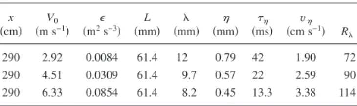
TABLE I. Evolution of the turbulence characteristics for the single phase flow for three different velocities at our measurement volume location. x: distance downstream the grid; V0: mean longitudinal velocity;⑀: dissipation
rate; L,, and: integral; Taylor and Kolmogorov length scales,;v: Kolmogorov time and velocity scales; and the last column displays the Taylor scale based Reynolds number.
x 共cm兲 V0 共m s−1兲 共m2⑀s−3兲 L 共mm兲 共mm兲 共mm兲 共ms兲 v 共cm s−1兲 R 290 2.92 0.0084 61.4 12 0.79 42 1.90 72 290 4.51 0.0309 61.4 9.7 0.57 22 2.59 90 290 6.33 0.0854 61.4 8.2 0.45 13.3 3.38 114
slowly than jw
3
so that in the end seeding density C0
⬀g共jw兲−3is a decreasing function of water flow rate jw. Since
particles are injected in the convergent part of the tunnel, upstream the grid for low wind velocities 共typically V0
ⱕ4 m s−1兲, the velocity in the convergent is not sufficient
for the heavier particles to reach the grid and they all settle before entering the fast section of the tunnel. This results in a severe decrease of particles diameters observed in experi-ments at fixed air pressure and water flow rate for low wind velocities. We have shown that above V0⯝4 m s−1, particles
diameter distributions in the measurement region are not much affected by the wind velocity. Once particles diameter distributions are obtained for a given set of injection param-eters, we build a corresponding most probable Stokes num-ber defined as St=共dmax/兲2共1+2⌫兲/36, where dmax
corre-sponds to the maximum of diameters distribution 关see Fig.
2共e兲兴. Figure2共f兲represents the evolution of dmaxas a
func-tion of air pressure and water flow rate in the nozzles for a given carrier flow Reynolds number. We stress that because of the high polydispersity the standard deviation St of
Stokes number共based on measured diameters distribution兲, which could be interpreted as an error bar for the Stokes number estimation, is large共St/St easily exceeds 50%兲 and
will not be displayed on the figures presented in the sequel. To summarize, each experiment is characterized by the set of parameters 共R, St, C0兲 with R, the carrier flow
Reynolds number共based on Taylor microscale兲, St, the aver-age Stokes number obtained as described above, and C0, the
global seeding density共which we cannot accurately measure, but which we assume to be directly related to the number of particles per image兲. Another usual relevant parameter is the Rouse number共defined as the ratio of the terminal velocity of the particles to the turbulent fluctuations intensity兲, which in our experiments, varies in a relatively narrow range from 0.4 to 2. A total of 90 experiments covering a set of about 40 different parameters triplets共R, St, C0兲 have been explored in order to investigate systematic effects on preferential con-centration phenomenon. In this study, we focus mainly on the influence of St and C0.
B. Acquisitions and postprocessing
Acquisitions are performed using a Phantom V12 high speed camera 共Vison Research, USA兲 operated at 10 kHz and acquiring 12 bits images at a resolution of 1280 pixels⫻488 pixels corresponding to a 125 mm 共along x兲⫻45 mm共along y兲 visualization window on the axis of the wind tunnel共covering slightly less than an inte-gral scale in the vertical y direction and almost two inteinte-gral scales in the streamwise x direction兲, located 2.95 m down-stream the grid. The camera is mounted with a 105 mm macro Nikon lens opening at f/D=2.8. An 8 W pulsed
2 3 4 5 6 0.03 0.04 0.05 0.06 0.07 0.08
injector air pressure
Vx fluctuation rate 2.3 m/s 3.9 m/s 7 m/s −6 −4 −2 0 −30 −20 −10 0 10 20 30 Vx(m.s -1) y (mm) V0=6.3 m.s-1 V0=4.5 m.s-1 V0=2.9 m.s-1 −6 −4 −2 0 −30 −20 −10 0 10 20 30 Vx(m.s -1) y (mm) 100 101 102 103 0 2 4 6 8 10 12 droplet diameter (μm) PDF (volume) x 1 0 -3 P=5 P=4 P=3 P=2 2 3 4 5 1 1.2 1.4 1.6 1.8 2
air pressure (bar)
water flow rate (l/mn) 50 60 70 80 90 100 100 101 102 103 10−9 10−8 10−7 10−6 10−5 10−4 10−3 10−2 k [m−1] PSD −5/3 (b) (a) (c) (d) (f) (e)
FIG. 2.共Color online兲 共a兲 Evolution of the ratio of tur-bulent fluctuations共Vrms兲 to mean wind velocity 共V0兲
both measured from from hot-wire anemometry as a function of the injector pressure without water flow 共note that the impact of the injectors on the turbulence level would even be lower with the presence of water兲 for three different mean velocities共equivalent turbulent fluctuation rate is constant and of the order of 3.5% when no air is blown in the injectors兲. 共b兲 Mean axial velocity averaged over x in the measurement volume 共x苸关289–301兴 cm兲 obtained from PIV. 共c兲 Mean axial velocities at different locations x in the measurement volume共also from PIV兲. Different symbols correspond to different location, note that the mean velocity is al-most constant within the measurement volume.共d兲
Ve-locity spectrum in the measurement volume.共e兲
Par-ticles diameter PDF evolution with air pressure 共varying from 2 to 5 bars兲 at fixed water flow rate 共1.2 l/mn for each injector兲 and fixed wind velocity 共V0= 4.5 m s−1兲. Note that PDFs are given from
par-ticles volume共and not particles number兲. 共f兲 Evolution of the maximum of these PDF with water flow rate and air pressure at the same fixed velocity共V0= 4.5 m s−1兲.
copper laser synchronized with the camera is used to gener-ate a 2 mm 共i.e., 3–4兲 thick light sheet illuminating the field of view in the stream-wise direction. The camera is orientated with a 50° forward scattering observation angle with respect to the laser sheet to increase the light budget. The resulting deformations are compensated by a Scheimpflug mount. Each experiment consists in a 0.9 s ac-quisition of 9000 images共corresponding to the available on board memory storage of the camera兲 at fixed wind velocity, water rate and air pressure in the injectors. Particles are iden-tified on the recorded images as local maxima with intensity higher than a prescribed threshold. As a consistency test, we have checked that changing the threshold around the selected value does not impact significantly the number of particles found. The subpixel accuracy detection is obtained by locat-ing the particles at the center of mass of the pixels surround-ing the local maxima.
As already mentioned, our aim is to study particles con-centration fields in order to quantify preferential concentra-tion effects and to identify particles clusters if any. Usual approaches to do this consider the pair correlation function to quantify preferential concentration effects while a box count-ing method is preferred to access local concentration fields. We propose to use a single tool to tackle simultaneously these two problems: the Voronoï diagrams. Such a Voronoï diagram is the unique decomposition of two-dimensional 共2D兲 space into independent cells associated to each particle. One Voronoï cell is defined as the ensemble of points that are closer to a particle than to any other. Use of Voronoï dia-grams is very classical to study granular systems and has also been used to identify galaxies clusters. The Voronoï diagram computation is very efficient 共we use MATLAB algorithm兲
with the typical number of particles per image共up to several thousands兲 we have to process. Figures3共a兲and3共b兲show a raw acquired image as well as the located particles and the associated Voronoï diagram.
III. PREFERENTIAL CONCENTRATION EVIDENCE AND QUANTIFICATION
A. Voronoï diagrams: Properties and advantages Why use Voronoï tessellations? From the definition of
the Voronoï diagrams, it appears that the area A of a Voronoï cell is the inverse of the local 2D-concentration of particles; therefore, the investigation of Voronoï area field is strictly
equivalent to that of local concentration field. We recall that usually local concentration fields are obtained through box counting methods7 that shows several disadvantages: they are computationally inefficient and they require to select an arbitrary length scale共the box size兲, whereas in Voronoï dia-gram computation, no length scale is a priori chosen and the resulting local concentration field is obtained at an intrinsic resolution. Similarly, the pair correlation function only gives global 共nonlocal兲 information and is also associated to the choice of a length scale that spans the whole values of inter-est increasing dreadfully the computation time. Finally, an-other interest of Voronoï diagrams is that as each individual cell is associated to a given particle at each time step, thus tracking in a Lagrangian frame the particles directly gives access to the Lagrangian dynamics of the concentration field itself along particles trajectories. Although we will not dis-cuss such Lagrangian aspects in this article, they represent an important opening which will be addressed in forthcoming studies.
Some relevant properties of Voronoï diagrams. Whatever
the measurement and data analysis technique used, when one refers to preferential concentration, it is implicitly assumed that one deals with statistical preferential concentration com-pared to the case where particles would be spatially distrib-uted as a random Poisson process共RPP兲. In order to quantify preferential concentration, we therefore compare for each ex-periment the probability density function共PDF兲 of the mea-sured Voronoï areas to that expected for a RPP. The main known properties of Voronoï diagrams associated to RPP can be found in a short review by Ferenc and co-worker18 and references herein. The first moment of Voronoï area PDF has nothing to do with the spatial organization of the particles since the average Voronoï area A¯ is always identical to the mean particles concentration inverse. Therefore, in the se-quel, we will generally focus on the distribution of the nor-malized Voronoï areaV=A/A¯ that is of unit mean. The only known exact result for RPP Voronoï areas statistics concerns the second order moment in the 2D case that is equal to 具V2典
RPP= 1.280 corresponding to a standard deviation VRPP
=
冑
具V2典RPP− 1⯝0.53. Regarding the shape of the PDF of
Voronoï areas statistics for a RPP, no analytical solution is known共most of the authors fit them with Gamma distribu-tions兲. Ferenc and co-worker proposed a compact analytical expression involving the space dimension as a single param-eter. We use this analytical expression as a RPP reference.
B. Experimental Voronoï area PDF
From instantaneous to statistical results. After
postpro-cessing the data as explained in Sec. II B, we obtain for each experiment 关corresponding to a given set of control param-eters共R, St, C0兲兴 a Voronoï diagram at each acquisition time
step. Due to the finite size of the field of view, the cells at the border of the diagram have infinite areas. We reject these border cells and keep only the particles whose Voronoï cell is fully included in the visualization window. To improve the statistical convergence of Voronoï area PDF estimation, we compute Voronoï diagram statistics from several uncorre-lated images from a given experiment. The unit mean
nor-100 200 300 400 400 500 600 700 x (pixels) y (pixels) 10 20 30 40 50 40 50 60 70 x (mm) y (mm) (b) (a)
FIG. 3. Left: a typical raw image. Right: particles located in this image and the associated Voronoï diagram. For clarity, we show only one third of the full acquired image.
malization共V=A/A¯兲 may then be performed for each image individually or for the whole set of images. We have checked that the impact of the normalization process is negligible. Figure6共a兲shows Voronoï area PDFs associated to ten dif-ferent statistical sets obtained by gathering 500 uncorrelated instantaneous Voronoï diagrams共UIVD兲 from a same experi-ment. The dispersion between the ten samples is quite small indicating that a good statistical convergence is already reached with 500 UIVD, except maybe in the extreme tails of the PDF. We find that the statistical convergence of the two first moments of these distributions is indeed achieved with one set of 500 UIVD. In the sequel, detailed PDF analy-sis was usually calculated using one set of 5000 UIVD from each experiment, while statistical error bars on second order moments for a given experiment关for instance, for the stan-dard deviation of Voronoï areasVin Fig.5共a兲兴 are estimated from the dispersion when these 5000 UIVD are split into ten sets of 500 UIVD analyzed individually.
Experimental Voronoï area distributions. Figure4共a兲 dis-plays the PDFs of the dimensional Voronoï cells area A for 40 different experiments. When the dimensional area A is considered, one observes that the maximum of these PDFs spans over 2 decades. This evolution is representative of the average number of particles per image共or equivalently of the global seeding concentration C0兲 that for the ensemble of
experiments represented goes from 50 to 5000. Note that as the average number of particles per image decreases共i.e., as the mean Voronoï area increases兲, the scattering of the right tail on these PDFs increases as a consequence of the lesser
statistical convergence. The same PDFs for the normalized Voronoï area V=A/A¯ collapse somehow 共not shown兲. The tails associated to large Voronoï areas, i.e., to regions of low particles concentration, actually collapse within measure-ments uncertainty, whereas the tails associated to relatively small Voronoï areas, i.e., to the regions of high particle centration show a much stronger dependency with the con-sidered experimental conditions, and particularly with the Stokes number as shown in Fig.4共b兲. Concerning the Rey-nolds number dependency, the robustness of PDF right tails 共associated to depleted regions兲 may be interpreted as the fact that the integral scale of the carrier flow is found not to change much when Ris increased共on the contrary the dis-sipation scale does decrease significantly兲. If large depleted regions are mostly associated to large eddies whose size is not affected when Ris increased, the distribution of Voronoï areas in these large depleted regions may also be expected to remain robust as Reynolds number changes. It is more diffi-cult to comment on the Rdependency of the PDF left tails 共associated to dense regions兲 for two reasons. The range of Reynolds numbers tested is narrow and St and Rare very correlated共see I兲 so that sets of experiments who span the explored range of Reynolds numbers at fixed St and C0 are
too scarce to be conclusive. Nevertheless, we observe changes in the PDF left tails with the Reynolds number that deserves a more thorough study we may undertake. The de-pendency on Stokes number is more subtle and is analyzed in the next paragraph.
While Voronoï area PDF of RPP are usually described by Gamma distributions,18 Fig.4共c兲shows that, for the inertial particles we investigate, Voronoï areas statistics are well de-scribed by a log-normal distribution. As seen on the figure, the superimposition with a log-normal distribution is almost perfect in the interval⫾2log共V兲, wherelog共V兲stands for the
standard deviation of log共V兲 共note that extreme PDF tails for statistics of the logarithm of V are beyond experimentally accessible statistical convergence兲. Log normality is further tested in Fig. 4共d兲 via the well-known log-normal relations between the two first statistical moments ofV and log共V兲
log共V¯兲 = log共V兲 +log共V兲2 /2, 共1兲
V2=V¯2共elog2 共V兲− 1兲, 共2兲
whereVstands for the standard deviation of the normalized areaV, and where by definition mean normalized area V¯=1. In this figure, each point for each plotted relation corre-sponds to each of the 90 carried experiments evidencing the very good verification of log-normal scaling共1兲and the rela-tively good verification of relation 共2兲 that is much more severe considering the difficulty to reach statistical conver-gence for logarithm of second moments. At the first order, we can therefore reasonably assume normalized Voronoï ar-eas to be log-normally distributed. To date, we do not have any theoretical interpretation of this log-normality, but this result shows that in the limit of experimental convergence, normalized Voronoï area PDFs can be described with one
10−1 100 101 102 103 10−6 10−5 10−4 10−3 10−2 10−1 100 A (mm2) PDF 10−2 100 102 10−4 10−2 100 PDF St=0.7 St=0.9 St=1.3 St=1.7 100 100 V = A/A −4 −2 0 2 4 10−4 10−3 10−2 10−1 100
(log(V) - log(V)) /σlog(V)
PDF 0 0.2 0.4 0.6 0.8 1 0 0.2 0.4 0.6 0.8 1 σ2 log(V) ( ) −log( V ) & ( ) log( σV 2+1) (b) (a) (c) (d)
FIG. 4.共a兲 PDF of dimensional Voronoï area A for 40 experiments spanning all R, St, and the volume loading explored.共b兲 PDF of normalized Voronoi area A/A¯ for four experiments at R⯝96 with varying Stokes number 共each PDF is calculated from 5000 instantaneous fields兲; inset displays a zoom around the maximum.共c兲 Centered and normalized PDF of the logarithm of Voronoï area for the 40 experiments from upper figure; black dashed line represents a Gaussian distribution.共d兲 Test of the log-normal scalings 共1兲 共gray dots兲 and 共2兲 共black dots兲 on 80 experiments spanning all R, St, and
C0; one point corresponds to one experiment. IfV has a log-normal
distri-bution, the dots should gather on the dash-dotted lines. Relation共1兲is very well verified; relation共2兲deviates slightly from the lognormal scaling, but is still relatively well verified considering the severeness of the test that in-volves second order moments of the variable logarithm for which statistical convergence becomes challenging.
single scalar quantity that we choose here to be the standard deviation of the normalized Voronoï areasV.
Quantifying preferential concentration. It is generally
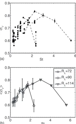
as-sumed that preferential concentration is primarily governed by particles Stokes number. Most former numerical and ex-perimental studies have evidenced that preferential concen-tration effects are more significant as the Stokes number ap-proaches unity. In Figs. 5共a兲 and 5共b兲, we present the evolution of the normalized Voronoï area standard deviation
V as a function of Stokes number in our experiments. In
Fig.5共a兲, each point corresponds to one single experiment. Lines connect different experiments for which the Reynolds number and the number of particles per image are kept con-stant. In Fig. 5共b兲, only the Reynolds number is constant along the lines, and each point is the average of points from the previous plot corresponding to experiments with the same Stokes number but possibly different number of par-ticles per image共error bars represent the dispersion between such experiments兲. As mentioned earlier, the standard devia-tion of Voronoï areas for a RPP is analytically known to be
VRPP⯝0.53 that defines a reference value to compare with. A
standard deviation V significantly exceeding 0.53 reveals the existence of high and low concentration events compared to the RPP case. Oppositely, a standard deviationV below this reference value would evidence the tendency of particles to distribute in a more organized arrangement共V= 0 in the limit of a perfect crystal兲. As seen on Figs.5共a兲and5共b兲, for the range of explored Stokes numbers共spanning from 0.2 to
almost 6兲, the standard deviation of the normalized Voronoï areas always exceeds 0.57 and reaches values as high as 0.85, which shows that preferential concentration is always present over this range of Stokes numbers, consistently with former experimental and numerical investigations. Further-more, both figures peak around Stpk⯝2–3 that is consistent
with the generally assumed feature that preferential concen-tration is maximal for Stokes number around unity corre-sponding to a better adjustment of particles response time to turbulence forcing time. In order to compare our Voronoï analysis with usual tools, we have also performed the box counting and correlation dimension analysis共not shown兲 that are consistently found to give a maximum effect of prefer-ential concentration also for Stpk⯝2–3. Figure 5共b兲 also suggests a possible Reynolds number effect as the curve for
R= 90 seems more peaked than curve at R= 114 and ap-pears to reach its maximum for a slightly lower value of Stpk.
However, one can hardly be conclusive on such a Reynolds number effect as it is mainly supported by only one point on the R= 90 curve关point St=2.2; 具V= 0.6典 in Fig.5共b兲兴 that furthermore presents relatively large statistical error bars. The possible specific influence of Reynolds number on pref-erential concentration will be addressed more deeply in forthcoming investigations. Moreover, as discussed in the following, the precise shape of trends in Figs.5共a兲and5共b兲
might be slightly affected by a bias on the estimation of particles typical Stokes number and subsequently on the ex-act value of Stpk as well as the width of the curves. For
example, we find Stpkⲏ1 while other studies 共mostly nu-merical兲 suggest a maximum effect for St⯝1. This might be attributed to an overestimation of the typical Stokes number of particles in our experiments as the actual turbulent dissi-pation scales 共 or 兲 might be slightly smaller than the values reported in TableIdue to the slight turbulence level enhancement from the spray injection process as described in Sec. II A共measurements in Table I, used for St estimation, were performed for the carrier flow alone, with particles in-jectors off, since accurate measurements of turbulence dissi-pation scales cannot be done at present with the sprays on兲. An increase of the actual turbulence level by 30%共as typi-cally observed when the nozzles blow only air but no water is injected兲 would, for instance, reduce by a factor of 2 the Stokes number estimation bringing Stpk to a value closer
to 1.
Finally, we also note that since our experiments cover a wide range of particles seeding concentrations, it is neces-sary to avoid any possible statistical bias onVdepending on the number of particles per image that are processed. This is a requirement forV to be considered as an actual quantita-tive indicator of preferential concentration. For instance, ex-periments with large particles关large Stokes numbers in Figs.
5共a兲and5共b兲兴 generally have less particles per image
共typi-cally less than 1000 ppi兲 than experiments with smaller par-ticles共which typically have 3000–4000 ppi兲. To test such a possible bias, we have estimatedVfrom a set of originally highly loaded images from which we randomly removed par-ticles. We have shown that the estimation ofVis extremely robust and not biased by this subsampling procedure as it is
0 2 4 6 0.5 0.6 0.7 0.8 0.9 St σV (a) 0 2 4 6 0.5 0.6 0.7 0.8 0.9 St R λ=72 R λ=90 R λ=114 <σ V > (b)
FIG. 5. Standard deviation of Voronoï areas as a function of average Stokes number.共a兲 One point corresponds to one single experiment, lines connect different experiments for which Reynolds number and the number of par-ticles per image is identical.共b兲 Only the Reynolds number is constant along lines, and each point is estimated as the averaged standard deviation from experiments with same Stokes number共but possibly different C0兲. Error bars represent the dispersion between such experiments.
only reduced by less than 1.5% when up to 80% of the par-ticles are randomly removed from the images.
As a partial conclusion, we emphasize that Voronoï analysis allows to robustly quantify preferential concentra-tion with a single scalar quantity共the standard deviation of normalized Voronoï areas兲 that is easily accessible and effi-ciently computed. This analysis confirms the trend of inertial particles to preferentially concentrate with a maximal effect for particles with Stokes number of order unity. However, we note that Voronoï area PDF on their own do not contain any information concerning the spatial structure of particles con-centration field that is a key point for the study of clustering and of its dynamics. In Sec. III C, we show how Voronoï area distributions can nevertheless be used to analyze the concen-tration field structure and dynamics.
C. Toward clusters identification and characterization from Voronoï analysis
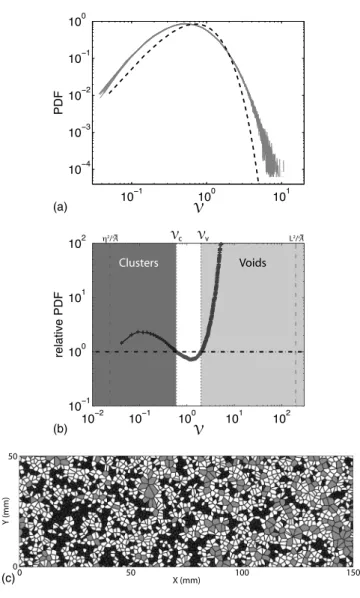
The Voronoï area PDF may be used to identify clusters of particles as follows. Consider Fig.6共a兲that presents the superposition of the Voronoï PDF for a typical experiment and for a RPP. These PDFs intersect twice 关which is more visible on Fig.6共b兲showing the ratio of both PDFs兴. For low and high values of normalized Voronoï area corresponding to high and low values of the local concentration, experimental PDF is above the RPP one while we observe the opposite for intermediate area values. This is consistent with the intuitive image of preferential concentration. Inertial particle concen-tration field is more intermittent than the RPP with more probable preferred regions where concentration is higher than the Poisson case and subsequently also more probable
depleted regions where concentration is lower than in the
Poisson case. We consider these intersection pointsVcandVv
as an intrinsic definition of particle clusters and voids. For a given experiment, Voronoï cells whose area is smaller than the first intersectionVcare considered to belong to a cluster
while those whose area is larger than the second intersection
Vv are associated to voids. We insist on the fact that these
thresholds are intrinsically chosen experiment wise and vary from one experiment to another. In particular, their evolution with the seeding concentration C0 is affine. Figure6共c兲
dis-plays a full Voronoï diagram corresponding to one image taken from one experiment. On this diagram, cells corre-sponding to clusters 共resp. to voids兲 have been colored in dark gray 共resp. light gray兲 while the remaining cells have been patched with white. It appears that dark gray cells共resp. light gray cells兲 tend to be connected in groups of various sizes and shapes that we identify as clusters 共resp. voids兲 whenever they belong to the same connected component.
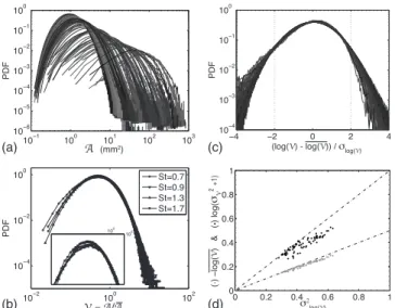
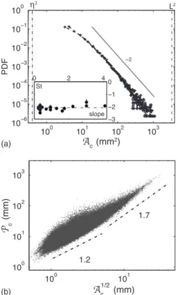
We then analyze the geometrical structure of the identi-fied clusters and voids. We have computed their area and perimeter from the area and perimeter of the constitutive Voronoï cells. We present the distributions of the clusters areaAcin Fig.7共a兲and the scatter plot of their perimeterPc
versusAc1/2in Fig.7共b兲. This last figure shows that for small and compact clusters,PcandAc
1/2are almost linearly related
while large structures exhibit a fractal behavior as also re-ported in previous experimental and numerical studies 共see
Ref.7and references herein兲. As shown in Fig.7共a兲, cluster areas Ac are found to be algebraically distributed with an
exponent⫺2 that is found to be independent of both Rand St within measurements accuracy共see inset兲. This interesting observation implies that clusters do not have a typical size 共not even an average兲. This result is contrary with the previ-ous study by Aliseda et al.7who fitted clusters area distribu-tions共measured from a box counting method兲 with a decay-ing exponential from which they could estimate a typical cluster size. However this estimation is questionable as the clusters area distributions they report are not clearly expo-nential and generally defined on so few points that an alge-braic behavior cannot be ruled out. We have performed the same analysis with the empty regions 共not shown兲 and we find very similar results than for clusters: large depleted re-gions have a fractal structure and their areas are algebraically distributed with an exponent close to⫺1.8. This last result is
10−1 100 101 10−4 10−3 10−2 10−1 100 V PDF (a) 10−2 10−1 100 101 102 10−1 100 101 102 V relative PDF Vc Vv Voids Clusters η2/A L2/A (b) 0 50 100 150 0 50 X (mm) Y (mm ) (c)
FIG. 6. A way to identify clusters.共a兲 Superposition of the Voronoï area PDF for a typical experiment共R= 85, St= 0.33, and C0= 500 particles per
image兲; ten continuous lines associated to ten sets of 500 UIVD are repre-sented共dispersion is negligible兲 and a RPP 共dotted line兲. 共b兲 Ratio of the two PDFs presented on the left figure. Vertical dash-dotted lines indicates2
共left兲 and L2共right兲. 共c兲 Colored visualization of clusters 共dark gray兲 and
voids共light gray兲.
in agreement with recent direct numerical simulations19 where void regions between inertial particles have been analyzed.
We now analyze the concentration within the clusters formerly identified. We define C, the mean concentration in-side a cluster, as the inverse of the mean Voronoï area within this cluster and C0 as the average particles concentration in
the whole images during one experiment共C0is the average
number of particles per image divided by the area of the whole visualization domain兲. Figure8共a兲presents the PDF of
C/C0 for nine typical experiments spanning our control
pa-rameters space. Though these PDFs are poorly converged due to an evident lack of statistics 共each identified cluster counts as one statistical sample兲 they are still well described, at first order, by a Gaussian distribution. Their means具C/C0典
define the averaged normalized concentrations within clus-ters for each experiment; it measures the average relative overloading of particles inside clusters. In our experiments, mean concentration in clusters is generally found to exceed twice the global seeding concentration and it can reach up to eight times the latter depending on experimental conditions 关see Figs.8共b兲and8共c兲兴. Figure 8共b兲shows the evolution of these mean normalized concentration with Stokes number, a globally growing trend with St can be seen, though scattering of data points is relatively large. On the contrary, as evi-denced in Fig. 8共c兲, the mean normalized concentration in clusters turns to be clearly dependent on the global seeding concentration C0 following a decreasing power law 具C/C0典
⬀C0−0.39. While one might have expected the concentration
inside the clusters to grow linearly with the global concen-tration 共具C/C0典 remaining constant兲 as a trivial geometric effect, this surprising decreasing power law dependency shows that the average concentration inside clusters grows more slowly than the global seeding concentration. As a con-sequence, the relative overloading of particles inside the clusters is reduced when the global seeding increases: for the lowest values of C0 clusters are up to 8 times overloaded
while they are only twice as dense as the average for the largest values of C0. To rule out any possible bias due, for
instance, to a statistical undersampling of low concentration experiments, we have performed the same whole analysis on artificially subsampled data: starting from the highest con-centration experiment共containing several thousands particles per image兲, we randomly removed up to 90% of the particles and we recomputed Voronoï tesselations and clusters identi-fication. We found that the algebraic distribution of clusters area is always maintained with the same −2 exponent, that the distribution of concentration within clusters is still Gaussian, and that mean normalized concentration in the clusters with the subsampled number of particles per image is weakly affected by the subsampling关see dots data on Fig.
8共c兲兴. This robustness of the analysis to arbitrary
subsam-pling shows that the effect observed in Fig.8共c兲does result from a physical process related to particles loading and not from a statistical bias.关We have also checked that this be-havior was not due to the definition of clusters we introduced based on the distance of Voronoï area PDF to RPP. Indeed, the same analysis was repeated for various fixed concentra-tion thresholds with respect to C0共which is the way clusters
are commonly defined in the literature兲, and the same law 具C/C0典⬀C0−0.39 was recovered.兴 Such a nontrivial effect,
which has never been reported to our knowledge, is therefore intrinsic to the clustering of dense particles by turbulence. It probably reveals the existence of collective effects inside the
100 101 102 103 10−6 10−5 10−4 10−3 10−2 10−1 100 Ac(mm 2) PDF 0 2 4 −3 −2 −1 0 St −2 slope η2 L2 (a) 100 101 100 101 102 103 Pc (mm) Ac (mm) 1/2 1.7 1.2 (b)
FIG. 7.共a兲 PDF of clusters area. The inset shows the evolution of the fitted power law exponent with Stokes number for the 40 experiments of Fig.4共a兲. Vertical dash-dotted lines indicates2共left兲 and L2共right兲. 共b兲 Geometrical
characterization of clusters for the same 40 experiments.
0 1000 2000 3000 0 2 4 6 8 C0(ppi) < C/C 0 > data subsampled power −0.39 0 1 2 3 4 5 0 2 4 6 8 St <C/C 0 > 0 1 2 3 4 5 0.8 0.9 1 1.1 1.2 1.3 St <C/C 0 >/F it (c) (a) (b) (d) −5 0 5 10-4 10-3 10-2 10-1 100 C/C0 PDF
FIG. 8. 共Color online兲 共a兲 PDF of normalized-reduced concentration C/C0
within clusters.共b兲 Evolution of the means of PDFs in figure 共a兲 with par-ticle Stokes number.共c兲 Evolution of the means of PDFs in figure 共a兲 with the global seeding concentration C0given in particles per image共䉮: all our
experiments,䊊: one single experiment randomly subsampled兲. 共d兲
Evolu-tion of the means of PDFs in figure共a兲 with the Stokes number after com-pensation by the seeding concentration dependance evidenced in figure共c兲.
clusters, and certainly deserves further investigations as well as cross-analysis with other experiments and numerical simulations. In particular, it should be underlined that this behavior is most probably not due to a steric effect. If so, one should expect both a linear increase of具C典 with C0 in the
dilute limit and a saturation of 具C典 共irrespective of C0兲 at
very large concentrations. None of these trends appear in Fig.8共c兲 共note that the concentration covers more than one decade in this figure兲.
Finally, we further check a possible dependency of 具C/C0典 on Stokes number 关which was not clearly visible at
first sight in Fig.8共b兲兴 by considering data on Fig. 8共b兲 di-vided by the empirical power law具C/C0典⬀C0−0.39 关obtained
from Fig.8共c兲兴 as a first attempt to separate Stokes number effects from the global seeding concentration effects just described. The result is presented in Fig.8共d兲 that shows a possible dependency on Stokes number with a maximum mean concentration in clusters occurring around St⯝2 remi-niscent of the maximum of preferential concentration ob-served in Figs.5共a兲and5共b兲. Although further investigations will be needed to be conclusive on this point, as discussed in Sec. IV, such a dependency can be consistently interpreted in the framework of a sweep-stick mechanism.20,21
IV. CONCLUSIONS AND OUTLOOKS
We have introduced the analysis of preferential concen-tration in turbulent particles laden flows using Voronoï dia-grams as a new tool to get a quantitative insight of the phe-nomenon. This very computationally efficient tool, not only gives access to the concentration field at an intrinsic local resolution共inverse of Voronoï areas directly gives local par-ticles concentration兲 but it also offers a remarkably simple and nonambiguous way to define particles clusters共as well as complementary voids兲 and to analyze their structural properties. Several known behaviors共previously reported in experimental and numerical works based on classical tools, mainly pair correlations, correlation dimension, and box counting兲, as the maximum of heterogeneity of the concen-tration field for particles with Stokes numbers around unity, have been successfully recovered and further analyzed at the light of this new tool. By systematically varying the triplet of parameters 共St,R, C0兲, we have shown that particles Voronoi’s area distributions are always reasonably log-normal, so that preferential concentration can be quantita-tively measured by a single scalar共the standard deviation of these distributions兲. We have characterized clusters 共and voids兲 geometries and their inner concentration. Geometrical properties共mainly the algebraic distribution of mean cluster areas and the fractal structure of clusters兲 may be interpreted as an evidence of the self-similar nature of preferential con-centration in particle laden flows. In particular, clusters do not appear to have any characteristic typical scale. The analysis of particle concentration inside the clusters has re-vealed two new and so far unpredicted results.
共i兲 The average particle concentration inside the clusters depends on the global particle loading in a nontrivial way.
共ii兲 After the compensation of this particle loading depen-dency, the average concentration inside the clusters exhibits a nonmonotonic dependency on the Stokes number with a maximum around unity values. To summarize Stokes number effects, we find that the overall preferential concentration is enhanced for particles with Stokes number around unity, cluster sizes, and geom-etries do not depend on Stokes number while mean concen-tration within clusters is also enhanced共at the second order when seeding concentration effects are decoupled兲 around unity Stokes numbers. All together, these results can be con-sistently interpreted in the framework of recently introduced sweep-stick mechanism by Vassilicos and co-workers.20,21 They propose a new physical process for the particle prefer-ential concentration phenomena where clusters form around zero acceleration points of the carrier flow to which particles tend to stick and to be advected with. These special points of the carrier flow have been thoroughly investigated in DNS20,21 and found to have at least two main remarkable properties: 共i兲 their spatial distribution is not uniform, and they tend to clusterize and共ii兲 inertial particles tend to stick to these points with an optimal stickiness for particles with Stokes number around unity. Physically, the sticking mecha-nism is dominated by the convergence of particles toward zero acceleration points along the maximum compression di-rection of acceleration gradients tensor of the carrier flow. This convergence is optimal when particles response timep
is of the order of the inverse of the corresponding contraction rate21 共if the response time is too small, contraction is too slow, while for too large response times contraction is fast but overshot by the particle inertia兲. In the context of the stick-sweep mechanism, cluster shape and size are therefore expected to be mostly prescribed by the carrier turbulence itself共in terms of clustering properties of zero acceleration points themselves兲. For instance, the fractal structure of zero acceleration point distribution has been identified in DNS.21 This is consistent with the self similarity we have observed in our experiment. In the same time, as a result of the Stokes number dependency of the stickiness of zero acceleration points, the concentration of particles within clusters is also expected in the context of this model to depend on Stokes number共with an optimum around St⬃1兲 and consequently so does the overall preferential concentration. This is also consistent with Stokes number trends observed experimen-tally. However some observations still remain to be under-stood. Yet, considering the sweep-stick mechanism alone, it is hard to qualitatively identify the origin of a departure from a linear increase of 具C典 with C0. Such a quantification re-mains to be done from available simulations.20,21 One possi-bility could be the indirect role of gravity 共gravity was not accounted for in the above mentioned simulations兲. Indeed, and in addition to the Stokes number, the Rouse number, which is the ratio of the terminal velocity to the turbulent intensity, is known to affect the behavior of particles in tur-bulence and in particular the preferential sweeping共see, for example, Ref. 22兲. In addition, particle-turbulence
interac-tions are known to enhance the settling velocity of dense inclusions.7,8,23One may expect that such a settling velocity
would tend to decorrelate somehow the particle locations from those of zero acceleration points, making clustering less efficient than expected. An argument in favor of such a sce-nario is that the enhanced settling velocity of inclusions in clustered regions is a collective effect that arises from the local concentration alone and thus is not Stokes dependent.7 In this framework, the influence of turbulence intensity on settling velocity enhancement is not completely clarified. If, as identified from simulations,8 this enhancement is propor-tional to the turbulence intensity, one may expect an evolu-tion of the relaevolu-tionship between具C典 and 具C0典 with Reynolds
number. Such a possibility is worth to be addressed in future investigations.
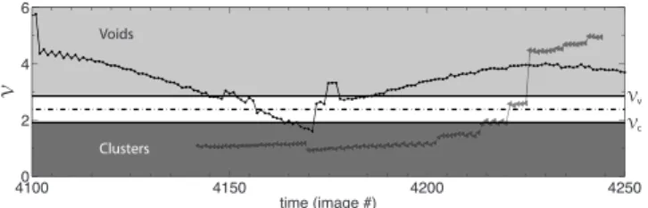
Similarly, a thorough comparative Voronoï analysis of zero acceleration points and particles clusters as well as a parametric Reynolds number study would shed more light on our results. The former is only accessible to numerical works so far, and regarding the latter, a drastic and challenging reduction of the polydispersity of the seeding fog is crucial for any experimental attempt. Numerical studies are natu-rally monodisperse and could also be of great help to this regard. Incorporating gravity effects in these simulations would also be useful regarding the question of the amount of demixing. To finish, we would like to stress the great poten-tial of Voronoï tesselations that offer a whole range of new openings for further investigations of particle laden flows. In particular, combined to classical Lagrangian particle track-ing, it allows to follow the local concentration in a Lagrang-ian frame共see Fig.9 that illustrates preliminary attempts of such Lagrangian local concentration tracking兲 giving simul-taneous access to statistics of particle dynamics共velocity and acceleration兲 and local concentration field around particles. Other important aspects concern clusters dynamics, and more specifically clusters lifetime as well as statistics of par-ticles residence time inside clusters共Lagrangian evolution of local concentration in Fig. 9 shows, for instance, two par-ticles traveling between clustered and void regions兲. Such conditional and dynamical information are expected to be key ingredients to improve our understanding and modeling capabilities for turbulent particle laden flows.
ACKNOWLEDGMENTS
This research is supported by ANR under the Contract No. ANR-07-BLAN-0155-04 共project DSPET兲. We would like to thank other members of this ANR project for fruitful discussions and Raphael Candelier for providing an efficient way to identify connected components.
1K. D. Squires and J. K. Eaton, “Preferential concentration of particles by
turbulence,”Phys. Fluids A 3, 1169共1991兲.
2J. K. Eaton and J. R. Fessler, “Preferential concentration of particles by
turbulence,”Int. J. Multiphase Flow 20, 169共1994兲.
3E. W. Saw, R. A. Shaw, S. Ayyalasomayajula, P. Y. Chuang, and Á.
Gylfason, “Inertial clustering of particles in high-Reynolds-number turbu-lence,”Phys. Rev. Lett. 100, 214501共2008兲.
4J. P. L. C. Salazar, J. de Jong, L. Cao, S. H. Woodward, H. Meng, and L.
R. Collins, “Experimental and numerical investigation of inertial particle clustering in isotropic turbulence,”J. Fluid Mech. 600, 245共2008兲.
5S. J. Scott, A. U. Karnik, and J. S. Shrimpton, “On the quantification of
preferential accumulation,”Int. J. Heat Fluid Flow 30, 789共2009兲.
6P. Olla, “Preferential concentration versus clustering in inertial particle
transport by random velocity fields,”Phys. Rev. E 81, 016305共2010兲.
7A. Aliseda, A. Cartellier, F. Hainaux, and J. C. Lasheras, “Effect of
pref-erential concentration on the settling velocity of heavy particles in homo-geneous isotropic turbulence,”J. Fluid Mech. 468, 77共2002兲.
8M. R. Maxey and J. J. Riley, “Equation of motion for a small rigid sphere
in a nonuniform flow,”Phys. Fluids 26, 883共1983兲.
9R. Gatignol, “The Faxen formulae for a rigid particle in an unsteady
non-uniform Stokes flow,” J. Mec. Theor. Appl. 2, 143共1983兲.
10E. Balkovsky, G. Falkovich, and A. Fouxon, “Intermittent distribution of
inertial particles in turbulent flows,”Phys. Rev. Lett. 86, 2790共2001兲.
11J. Bec, L. Biferale, G. Boffetta, A. Celani, M. Cencini, A. Lanotte, S.
Musacchio, and F. Toschi, “Acceleration statistics of heavy particles in turbulence,”J. Fluid Mech. 550, 349共2006兲.
12S. Ayyalasomayajula, A. Gylfason, L. R. Collins, E. Bodenschatz, and Z.
Warhaft, “Lagrangian measurements of inertial particle accelerations in
grid generated wind tunnel turbulence,” Phys. Rev. Lett. 97, 144507
共2006兲.
13R. Volk, E. Calzavarini, G. Verhille, D. Lohse, N. Mordant, J. Pinton, and
F. Toschi, “Acceleration of heavy and light particles in turbulence: Com-parison between experiments and direct numerical simulations,”Physica D 237, 2084共2008兲.
14N. M. Qureshi, M. Bourgoin, C. Baudet, A. Cartellier, and Y. Gagne,
“Turbulent transport of material particles: An experimental study of finite size effects,”Phys. Rev. Lett. 99, 184502共2007兲.
15N. M. Qureshi, U. Arrieta, C. Baudet, A. Cartellier, Y. Gagne, and M.
Bourgoin, “Acceleration statistics of inertial particles in turbulent flow,”
Eur. Phys. J. B 66, 531共2008兲.
16M. W. Reeks, “On probability density function equations for particle
dis-persion in a uniform shear flow,”J. Fluid Mech. 522, 263共2005兲.
17R. H. A. Ijzermans, M. W. Reeks, E. Meneguz, M. Picciotto, and A.
Soldati, “Measuring segregation of inertial particles in turbulence by a full
Lagrangian approach,”Phys. Rev. E 80, 015302共2009兲.
18J.-S. Ferenc and Z. Néda, “On the size distribution of Poisson Voronoi
cells,”Physica A 385, 518共2007兲.
19H. Yoshimoto and S. Goto, “Self-similar clustering of inertial particles in
homogeneous turbulence,”J. Fluid Mech. 577, 275共2007兲.
20S. Goto and J. C. Vassilicos, “Self-similar clustering of inertial particles
and zero-acceleration points in fully developed two-dimensional turbu-lence,”Phys. Fluids 18, 115103共2006兲.
21S. W. Coleman and J. C. Vassilicos, “A unified sweep-stick mechanism to
explain particle clustering in two- and three-dimensional homogeneous, isotropic turbulence,”Phys. Fluids 21, 113301共2009兲.
22C. Y. Yang and U. Lei, “The role of the turbulent scales in the settling
velocity of heavy particles in homogeneous isotropic turbulence,”J. Fluid
Mech. 371, 179共1998兲.
23L. I. Zaichik and V. M. Alipchenkov, “Statistical models for predicting
pair dispersion and particle clustering in isotropic turbulence and their applications,”New J. Phys. 11, 103018共2009兲.
41000 4150 4200 4250 2 4 6 time (image #) V Voids Clusters Vc Vv
FIG. 9. Voronoï area trajectories for two particles. The dashed-dotted hori-zontal line shows the cluster threshold defined above, the continuous lines are, respectively, 80% and 120% of this threshold. The track with triangles is clearly associated to a particle that is ejected from a cluster around