Surface mass balance model intercomparison for the Greenland ice sheet

(1)

The Cryosphere, 7, 599–614, 2013 www.the-cryosphere.net/7/599/2013/ doi:10.5194/tc-7-599-2013

EGU Journal Logos (RGB)

Advances in

Geosciences

Open Access

Natural Hazards

and Earth System

Sciences

Open Access

Annales

Geophysicae

Open Access

Nonlinear Processes

in Geophysics

Open Access

Atmospheric

Chemistry

and Physics

Open Access

Atmospheric

Chemistry

and Physics

Open Access Discussions

Atmospheric

Measurement

Techniques

Open Access

Atmospheric

Measurement

Techniques

Biogeosciences

Open Access Open Access

Biogeosciences

Discussions

Climate

of the Past

Climate

of the Past

Discussions

Earth System

Dynamics

Earth System

Dynamics

Discussions

Geoscientific

Instrumentation

Methods and

Data Systems

Open Access

_{Geoscientific}

Instrumentation

Methods and

Data Systems

Geoscientific

Model Development

Geoscientific

Model Development

Discussions

Hydrology and

Earth System

Sciences

Open Access

Hydrology and

Earth System

Sciences

Ocean Science

Discussions

Solid Earth

Discussions

The Cryosphere

Discussions

Natural Hazards

and Earth System

Sciences

Open Access

Discussions

Surface mass balance model intercomparison for the Greenland

ice sheet

C. L. Vernon1, J. L. Bamber1, J. E. Box2, M. R. van den Broeke3, X. Fettweis4, E. Hanna5, and P. Huybrechts6

1_{School of Geographical Sciences, University of Bristol, Bristol, UK}

2_{Ohio State University, Byrd Polar Research Center and Dept. of Geography, Columbus, Ohio, USA} 3_{Institute for Marine and Atmospheric Research Utrecht, Utrecht University, Utrecht, the Netherlands} 4_{Department of Geography, University of Liege, Liege, Belgium}

5_{Department of Geography, University of Sheffield, Sheffield, UK}

6_{Earth System Sciences and Department of Geography, Vrije Universiteit, Brussels, Belgium}

Correspondence to: C. L. Vernon (chris.vernon@bristol.ac.uk)

Received: 31 July 2012 – Published in The Cryosphere Discuss.: 20 September 2012 Revised: 7 March 2013 – Accepted: 8 March 2013 – Published: 3 April 2013

Abstract. A number of high resolution reconstructions of

the surface mass balance (SMB) of the Greenland ice sheet (GrIS) have been produced using global re-analyses data ex-tending back to 1958. These reconstructions have been used in a variety of applications but little is known about their consistency with each other and the impact of the down-scaling method on the result. Here, we compare four recon-structions for the period 1960–2008 to assess the consistency in regional, seasonal and integrated SMB components. Total SMB estimates for the GrIS are in agreement within 34 % of the four model average when a common ice sheet mask is used. When models’ native land/ice/sea masks are used this spread increases to 57 %. Variation in the spread of com-ponents of SMB from their mean: runoff 42 % (29 % native masks), precipitation 20 % (24 % native masks), melt 38 % (74 % native masks), refreeze 83 % (142 % native masks) show, with the exception of refreeze, a similar level of agree-ment once a common mask is used. Previously noted differ-ences in the models’ estimates are partially explained by ice sheet mask differences. Regionally there is less agreement, suggesting spatially compensating errors improve the inte-grated estimates.

Modelled SMB estimates are compared with in situ obser-vations from the accumulation and ablation areas. Agreement is higher in the accumulation area than the ablation area sug-gesting relatively high uncertainty in the estimation of abla-tion processes. Since the mid-1990s each model estimates a decreasing annual SMB. A similar period of decreasing SMB

is also estimated for the period 1960–1972. The earlier de-crease is due to reduced precipitation with runoff remaining unchanged, however, the recent decrease is associated with increased precipitation, now more than compensated for by increased melt driven runoff. Additionally, in three of the four models the equilibrium line altitude has risen since the mid-1990s, reducing the accumulation area at a rate of ap-proximately 60 000 km2per decade due to increased melting. Improving process representation requires further study but the use of a single accurate ice sheet mask is a logical way to reduce uncertainty among models.

1 Introduction

The Greenland ice sheet (GrIS) is the world’s second largest single ice mass representing approximately 7 m of sea level rise were it to melt entirely. Whilst it contains only an eighth of the mass of the Antarctic ice sheet, the GrIS is important to study since surface melting is already intense (estimated in excess of 1 m water equivalent) along its margins (Fettweis, 2007). Further, the susceptibility to Northern Hemisphere po-lar amplification makes this ice sheet particupo-larly vulnerable to future climate change.

The mass balance of an ice sheet is its time-varying rate of change of mass and is an important measure of its “state of health”. It can be determined from the sum of two terms: the solid ice discharge to the ocean and the surface mass

(2)

balance (SMB), with a minor contribution from basal melt (Huybrechts et al., 2011). The SMB is the sum of the surface mass gain by precipitation (solid ice and liquid) and water vapour deposition (collectively termed: accumulation) and mass loss from the surface by runoff and sublimation (col-lectively termed: ablation). For the ice sheet to be in mass balance, the ice lost through ice flow discharge from the ice sheet must be matched by mass gain from SMB. For the GrIS this was identified to be the case between 1971 and 1988 (Rignot et al., 2008); however, from the mid-1990s there has been an increase in both solid ice discharge and runoff, resulting in the GrIS losing mass at an accelerating rate (Velicogna, 2009; Rignot et al., 2011). These two in-creases attributed to ice dynamics and surface processes have contributed approximately equally to recent mass loss (van den Broeke et al., 2009).

Estimating the mass balance of the ice sheet from the sum of SMB and discharge is termed the mass budget or input-output method (Rignot et al., 2011) and the errors in this approach are generally dominated by uncertainties in SMB. Mass budget estimates have, in the past, used the SMB recon-structions that are discussed here (Rignot et al., 2008, 2011; van den Broeke et al., 2009) and relied on the error estimates from these studies. It is, however, difficult to determine errors in downscaling models and numerical models of the climate system in general (Stephenson et al., 2012), especially when, as is the case here, validation data are limited in space, time and accuracy. A model intercomparison exercise is useful, in such circumstances, to identify the degree of consistency in spatial and temporal (seasonal-decadal) patterns between the models and to determine whether the differences are con-sistent with the quoted errors. In some instances, a multi-member ensemble can have greater model skill than any in-dividual reconstruction (Overland et al., 2011). Comparison with independent validation data can also provide insights into the behaviour of the different methods. Here, we exam-ine four reconstructions, all driven, by a common forcing: The European Centre for Medium Range Weather Forecast-ing (ECMWF) re-analysis data. We compare seasonal, inter-annual and regional estimates of various components of the SMB to examine the impact of the downscaling methodol-ogy on the modelled parameter and to quantify the degree of consistency between the approaches. In this study, we do not attempt to propose a preferred approach or data set because (i) the independent validation data used here are inadequate for this purpose, and (ii) different components of the SMB, for different regions, may have different levels of skill be-tween the approaches and it depends, therefore, on the met-ric of interest as to which is considered more reliable. Irre-spective of this limitation, it should be stressed that excellent progress has been made over about the last decade in mod-elling the SMB of the GrIS. Surface processes are now cap-tured, over the whole ice sheet, at length scales down to 5 km, and with time steps that accurately represent the diurnal cy-cle in temperature and radiation fluxes and the seasonal cycy-cle

of mass fluxes (van den Broeke et al., 2009). The reasonable agreement between three different approaches for determin-ing the time-evolvdetermin-ing mass trends for the ice sheet suggests that the SMB reconstruction used must be relatively robust in terms of temporal, and large scale regional, trends (Sasgen et al., 2012). Thus, although validation data for runoff and ablation processes (including refreezing) are sparse and limit our ability to test the simulations in the ablation zone, confi-dence in the quality and reliability of the reconstructions can be gained from inter-comparisons such as that undertaken by Sasgen et al. (2012). In addition, improvements to the models are being continuously made.

GrIS SMB has been estimated through the statistical downscaling of low resolution re-analysis data Hanna et al. (2011, 2005, 2002, 2008), and low resolution global cli-mate model data (Huybrechts et al., 2004; Gregory and Huy-brechts, 2006) through regional climate models (Box et al., 2004, 2009; Ettema et al., 2010a, b; Fettweis, 2007; Fettweis et al., 2008; Lucas-Picher et al., 2012) and also through the interpolation of in situ observations from ice cores, snow pits, stake measurements and automatic weather stations (Bales et al., 2009); however, these measurements are limited in both spatial and temporal coverage and are unable to separate components of SMB. The release of high-quality and consis-tent historical weather reanalysis data has made possible the modelling of the processes controlling SMB over the whole ice sheet. Temporal differences between these SMB estima-tions have been identified (Dahl-Jensen et al., 2009; Rae et al., 2012) yet remain to be explained. Here we consider four such reconstructions of GrIS SMB carried out using a com-mon forcing: re-analysis data from ECMWF.

The purpose of this study is to elucidate the differences in SMB estimation arising from different models forced with common forcing data in order to assess their consistency be-tween models and against their quoted errors. We compare these reconstructions, with a focus on ice sheet mask choice, annual time series and the seasonal cycle over the period 1960–2008 to each other and to in situ data where they are available.

1.1 Modelling approach

The annual specific SMB is defined as net accumulation mi-nus net ablation during a year:

SMB = P − TMT − R, (1)

where P =precipitation; TMT = turbulent moisture transport (evaporation, sublimation and deposition) and

R =runoff.

Runoff is in turn defined as

R =Rain + M − RF − RE, (2)

where M is melt, RF is refreeze and RE is melt and rain water retention.

(3)

All components are quoted in units of mm water equiva-lent. Specific SMB is integrated over the ice sheet to give the total SMB, given in Gt yr−1_.

Each component of SMB can be estimated from the ECMWF global climatology re-analysis product known as ERA-40 (Uppala et al., 2005), a data assimilation product covering the period 1957–2002 produced by re-analysing historic observations using a consistent weather prediction model. After 2002 either ERA-INTERIM (Dee et al., 2011) or operational analysis is available up to the recent past. As ERA-40 is not available over the recent years, we need to use two different forcing products (first ERA-40 followed by ERA-INTERIM or operational analysis) and inhomogeneity can occur between the two data sets due to changes in the as-similation procedure or in the data availability over the study period (1960–2008). In addition the observational record for Greenland is relatively poor so ERA-40 is more strongly in-fluenced by the ECMWF atmospheric forecast model used during data assimilation. ERA-40 uncertainty is therefore likely to be larger over Greenland than other areas.

With a resolution of ∼ 110 km, ERA-40 is relatively coarse to be used directly to estimate GrIS SMB. SMB is dependent on smaller scales due primarily to the narrow ab-lation area (with a typical width of 10–100 km) but more generally the topographic length scale. One approach, em-ployed by Hanna et al. (2002, 2005), downscales surface air temperature and precipitation to a higher resolution. We call this approach ECMWF-downscale (ECMWFd). A sec-ond approach, employed independently by Box et al. (2006, 2009), Fettweis (2007) and Ettema et al. (2010a, b) uses high resolution regional climate models (RCMs) as physically-based interpolators of the re-analysis climatology.

Concern has been raised about the suitability of ERA-40 and subsequent operational analysis for Arctic studies fol-lowing the discovery of a discontinuity in mid- to lower tro-posphere air temperatures in 1997 (Screen and Simmonds, 2011). It remains to be seen what, if any, impact this result has on SMB modelling of the GrIS. Other reanalysis prod-ucts are available and some have been used to force RCMs over the GrIS but, with the aim of eliminating an “external” source of variability in the analysis, only the four models detailed below that employ ECMWF re-analyses have been compared here.

2 Model and data description

2.1 Polar MM5

The Polar Pennsylvania State University (PSU) – National Center for Atmospheric Research (NCAR) Fifth-Generation Mesoscale Model (Polar MM5) is a regional climate model coupled to a surface snow model, with a horizontal resolution of 24 km. The realisation of the model used for this study is described in Box et al. (2009).

The model is forced at its boundaries every 6 h with ERA-40 to 2002, thereafter 12 hourly operation analysis data. The model is reinitialised every month. Tests indicated that the difference in the time interval of the forcing data did not in-troduce any inconsistency in the downscaled product. Addi-tionally, no significant difference was seen between ERA-40 and operational analysis for overlapping periods (Box et al., 2009). Melting is modelled by an energy balance model (EBM) including model bias correction based on in situ data. The amount of melting, M, is related to the amount of resid-ual energy, QM, as

M = QMt (Lρ)−1, (3)

where t is time, ρ is ice density and L is the latent heat of fusion. Thus QM is calculated as

QM=QN−(QH+QE+QG+QR), (4) where QN is the net radiative flux, QH and QE are the turbulent sensible and latent heat fluxes, respectively, QG is the firn/ice conductive heat flux and QR is the sensible heat flux from rain. Runoff is calculated using the Pfeffer et al. (1991) meltwater retention and refreezing parameterisa-tion with runoff occurring when surplus water is free to per-colate downslope once firn is saturated. This model is lim-ited in scope to a single season’s accumulation layer, so may overestimate runoff in warm years as meltwater is unable to percolate into the earlier year’s accumulation. A three hourly model output is integrated to produce monthly distributions of SMB components.

In the period 2000–2008 surface albedo observations from the NASA Terra platform (MODIS) sensor MOD10A1 prod-uct (Hall et al., 2011; Stroeve et al., 2006) were updated daily when grid cells were determined by the data prod-uct to be clear sky. In the 1981–1999 period, albedo from the 1981–2000 period based on AVHRR APP-x data (Key et al., 2006) is prescribed. Prior to 1981, multi-year (2000– 2008) daily averaged MODIS MOD10A1 albedo data are prescribed.

2.2 RACMO

The Regional Atmosphere Climate Model version 2.1 (RACMO2.1) was developed by the Royal Netherlands Me-teorological Institute (KNMI) (van Meijgarrd et al., 2008). Adjustments specific to the Arctic environment have been made to the original model to produce RACMO2/GR. The regional climate model with a resolution of approximately 11 km, is forced at its boundaries by ERA-40 (followed by operational analysis after August 2002) every 6 h and evolves freely within the model domain. Sea surface temperature and sea ice open fraction are prescribed. The model is described by Ettema et al. (2010a, b).

In addition to the atmosphere model, an energy balance snow metamorphism model is required for the calculation

(4)

of SMB components (excluding precipitation). The RACMO atmosphere model is coupled to an energy balance model, described by Bougamont et al. (2005), to calculate T , the surface temperature and thus the melt energy, ME:

ME=SW↓(1 − α) + εLW↓−εσ T4+QH+QE+QR, (5) where ME=melt energy, SW↓ and LW↓ are the

down-ward fluxes of solar and longwave radiation, α = albedo and

ε =surface emissivity. T is used as the boundary condition for temperature modelling through the snow/firn/ice layer. Albedo is a function of snow density and cloudiness.

The subsurface multi-layer snow model is based on the SOMARS model (Simulation Of glacier surface Mass balance And Related Sub-surface processes) described by Greuell and Konzelmann (1994). Here temperature diffuses vertically through the column and surface melt and rainwater percolate downward. Refreezing increases subsurface tem-peratures and density, which cannot exceed the melting point or the density of ice. Remaining water after these constraints are met percolates to the next layer with a small proportion held by capillary forces. Upon reaching an impermeable ice layer, pore space is filled to form a slush layer and liquid runoff is generated from an exponential decay of slush con-tent as a function of surface slope. This is the highest res-olution RCM considered in this study and has been shown to generate significantly more precipitation and higher SMB, suggested to be a result of capturing high accumulation peaks (Ettema et al., 2009).

2.3 MAR

Modèle Atmosphérique Régional (MAR) is a coupled atmosphere–snow regional climate model with horizontal resolution of 25 km. The atmospheric part is described by Gallee and Schayes (1994) and the surface component, SISVAT (soil, ice, snow, vegetation atmosphere transport), by De Ridder and Gallee (1998). As with RACMO a multi-layered energy balance snow model is employed to estimate meltwater percolation, retention and refreezing, snow densi-fication due to liquid refreezing and firn compaction. This model, called CROCUS, is notably described by Brun et al. (1992) and (Reijmer et al., 2012). Albedo is calculated differently to RACMO though. In addition to cloudiness and zenith angle, when snow depth exceeds 10 cm, albedo de-pends on the shape and size of the snow grains as described by CROCUS. However, for shallow snow cover, albedo varies linearly from snow to bare ice (α = 0.45) (Lefebre et al., 2003). Refreeze data have not been provided for MAR therefore has been generated as follows:

Refreeze = Melt + Rain − Runoff. (6)

Liquid water retention and evaporation data are not provided so it is included in the generated refreeze series.

As with RACMO2/GR and PMM5, MAR was forced ev-ery 6 h with temperature, humidity and wind fields from

ERA-40 and from 2002 onwards with ERA_INTERIM at the boundaries of its integration domain. Sea surface tempera-tures and sea ice cover were prescribed from the ECMWF re-analysis (Fettweis, 2007; Fettweis et al., 2005). However, unlike the PMM5 model, MAR is not recalibrated or cor-rected against in situ data. This iteration of MAR has no-tably been used in studies by Box et al. (2012), Reijmer et al. (2012) and Franco et al. (2012).

2.4 ECMWF-downscale

Unlike the previous three atmospheric models, the approach taken by Hanna et al. (2011, 2005, 2002, 2008) referred to here as ECMWFd does not model the atmosphere over Greenland. Instead ERA-40 and operational analysis surface air temperature, precipitation and surface latent heat flux are downscaled by bilinear interpolation from the original reso-lution of 1.125◦_{latitude × 1.125}◦_{longitude to a 0.5}◦_×_0.5◦

grid. Evaporation when temperatures exceed 0◦C and sub-limation for < 0◦C are calculated from the latent heat of vaporisation and sublimation, respectively. To model runoff on the narrow GrIS margin these downscaled fields are aver-aged monthly and further downscaled onto a 5 km grid before runoff is calculated. A correction is applied to the surface air temperature (SAT) field based on lapse rates to compensate for the often several hundred metre elevation error present in the relatively low resolution (∼ 110 km) ERA-40.

Runoff and refreeze is calculated with a positive degree day (PDD) driven parameterisation after Janssens and Huy-brechts (2000); therefore, correcting the SAT is important. Runoff is assumed to occur when melt exceeds a certain frac-tion of precipitafrac-tion so the model depends on SAT and pre-cipitation (Hanna et al., 2005). The fraction of prepre-cipitation falling as rain is calculated as proportional to the time frac-tion with SAT > 1◦C, with rainfall freezing if the snowpack is cold enough. Runoff only occurs once pores in the snow-pack are filled to a certain density and removes the snow plus capillary water. Melt of the ice can only occur once the snow is removed (Hanna et al., 2005). This PDD approach does not require albedo to be estimated. Refreeze fields have not been provided for ECMWFd so refreeze has been generated per Eq. (6).

Downscaled output is validated by in situ data collected by the Danish Meteorological Institute’s (DMI) weather sta-tions (Cappelen, 2011) and the Greenland Climate Network (GC-Net) of automatic weather stations (Steffen and Box, 2001). These data are used to derive the empirical lapse rates applied to the SAT field as it is downscaled to the 5 km grid. The calibration results in a good fit, with modelled SAT within 1 K of the observed for most weather stations, and larger deviations of ±3 K only occurring in a few loca-tions (Hanna et al., 2005). The authors note that the down-scaled temperatures for the runoff area are probably within several tenths of a degree of reality. One concern over this confidence is that the DMI data were assimilated into the

(5)

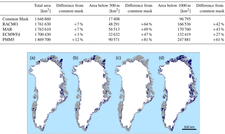
Table 1. Ice sheet mask area. Differences between each mask’s total area and the common mask are small, however, differences in the influential low elevation areas are significant.

Total area Difference from Area below 500 m Difference from Area below 1000 m Difference from [km2] common mask [km2] common mask [km2] common mask

Common Mask 1 646 860 17 408 96 795 RACMO 1 761 630 +7 % 48 291 +64 % 166 536 +42 % MAR 1 763 610 +7 % 56 513 +69 % 170 760 +43 % ECMWFd 1 700 430 +3 % 32 632 +47 % 132 419 +27 % PMM5 1 869 700 +12 % 90 571 +81 % 247 881 +61 % (a) (b) (c) (d) 500 km

Fig. 1. Four ice sheet masks. Areas in white are common to all masks, dark blue represents additional areas of each mask (a) RACMO, (b) MAR, (c) ECMWFd, (d) PMM5. Land area is shown in grey.

ERA-40 product so downscaled data are not independent from observations. The GC-Net data however remains in-dependent. The ECMWFd version used here is described in Hanna et al. (2011). A further RCM for the GrIS, HIRHAM5 (Lucas-Picher et al., 2012), is not considered here as esti-mates are only available over the period 1989–2009, forced by ERA_INTERIM.

The statistical downscaling model, SnowModel (Mernild and Liston, 2012), is also not considered for this study as modelled data forced by the common ERA-40 used for the other models are not available.

2.5 Mask variation

The four models use different ice sheet masks (Fig. 1). For ease of comparison each data set is regridded (with result-ing fractional grid boxes on the edge rounded to form a bi-nary mask) to a common projection and 5 km grid, a process which introduces small (∼ 1 %) changes from the native out-put. While the differences in area are relatively small with the largest ice sheet mask (PMM5, including all permanent ice) having an area 110 % of the smallest (ECMWFd, only the contiguous ice sheet), the difference is important because some areas of the ice sheet are more affected by certain

pro-cesses than others due primarily to their elevation. ECMWFd only models SMB on the ice sheet itself rather than marginal ice caps and glaciers. Low lying ice has a disproportional impact on the SMB and components of SMB (Hanna et al., 2005; Franco et al., 2012). The ice sheet area below 1000 m, well below the equilibrium line altitude (ELA), varies from 247 881 km2to 132 419 km2between models, a difference of 87 %. The scale of this mask variation is described in Table 1. To allow more meaningful model comparison in this work either a common mask, or a metric unaffected by mask vari-ation such as the ELA is used for subsequent analysis. The common mask is not closer to reality; it is very likely smaller than the GrIS but is a common denominator for model com-parison. However, this does not remove all variation as the different model resolution will affect how topography is rep-resented.

PMM5 uniquely uses a fuzzy mask. In this case clas-sification of the grid cells as permanent ice, land, ocean, and mixed “pixels” is made using 1.25 km resolution June– August NASA Moderate Resolution Imaging Spectrora-diometer (MODIS) bands 1–4 and 6, cloud-free imagery from 2006. The surface is considered permanent ice if sur-face reflectance exceeds 0.3 and if the normalised difference vegetation index is less than 0.1. When the 1.25 km grid is

(6)

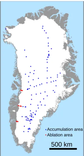
Accumulation area Ablation area

500 km

Fig. 2. Spatial distribution of in situ SMB observations.

interpolated to 5 km using a “nearest neighbour” basis to quantify how much mixing of the grid cells by land takes place, it is possible to define a “fuzzy” mask that quantifies the mixing of land and ice using a value between 0 and 1. As such, selection of a mask threshold to represent the aver-age case of permanent ice partially addresses the sub-grid is-sue while maintaining the ability to accurately determine the mass flux. Based on this classification, our best estimate of the permanent ice covered area tuned to match permanently glaciated areas reported by Kargel et al. (2011) corresponds with mask values greater than or equal to 0.587, resulting in an area of 1.824 × 106 km2. Non-ice sheet grid cells are ex-cluded from the reconstruction. There are 72 974 grid cells counted as glaciated. In all, 2496 of these grid cells are iso-lated from the inland ice sheet, totalling 62 393 km2.

2.6 Validation Data

Ice cores and snow pits are used to measure accumulation rates in the accumulation area. Bales et al. (2001, 2009) and Cogley (2004) have collated the available data. In the abla-tion area stake measurements are taken but due to the logis-tical difficulties of repeat visits there are fewer of this type

1960 1970 1980 1990 2000 2010 0 100 200 300 400 Max−Min (Gt) Common Mask Native Mask

Fig. 3. Spread between highest and lowest modelled SMB annual series on the common (141 Gt) and native (208 Gt) masks. Dashed lines indicate 1960-2008 mean.

of measurement. Here we only consider ablation area obser-vations along the K-transect, lying at approximately 67◦N in West Greenland (van de Wal et al., 2012).

Each observation provides an average yearly SMB over a several year period. After filtering temporally (1960–2008 period) and spatially (common mask) for the period and area under consideration, there are 101 observations above 1500 m in the accumulation area and five from the K-transect below 1500 m comparable with model estimates. In the ac-cumulation area, there is good temporal coverage throughout the period; however, observations from the ablation area are only from 1990 onwards. The locations of the in situ data are illustrated in Fig. 2.

3 Results

3.1 Impact of mask variation

Approximately a third of inter-model SMB variation can be explained by the large mask variation at low altitude (Fig. 3). Using a common mask did reduce the model differences for total SMB and most components of SMB. Figure 3 illus-trates the annual spread between highest and lowest mod-elled SMB annual series on the common (141 Gt mean) and native (208 Gt mean) masks. There is a smaller spread, indi-cating less difference between modelled output on the com-mon mask than the models’ individual masks. Moving to the common mask reduces mean inter-model spread by 67 Gt or 32 %. The remaining 141 Gt spread is 34 % of the four model mean annual SMB (411 Gt yr−1_{) on the common mask over} the 1960–2008 period. This compares to a spread of 57 % of the mean when the models’ native masks are used due to a larger spread (208 Gt mean) of a smaller four model average annual SMB (363 Gt yr−1). This observation hides some structure. On years with high SMB, RACMO and to a lesser extent MAR show higher SMB on their native larger masks than on the common mask, meaning the relatively low

(7)

Table 2. Average annual SMB on model’s native mask and the com-mon mask.

Model SMB (Gt yr−1) SMB (Gt yr−1) Difference 1960–2008 1960–2008

Native Mask Common Mask

RACMO 470 470 +0 %

MAR 401 432 +8 %

PMM5 301 404 +34 %

ECMWFd 279 340 +22 %

Mean 363 411 +13 %

altitude region, not included in the common mask, has a net positive SMB. This is not the case for PMM5 and ECMWFd where their native masks always produce lower SMB. This different response to the common mask increases the spread between models.

The spread is dominated by the high estimate of RACMO (470 Gt yr−1on both native and common masks) and the low estimate of ECMWFd (279 and 340 Gt yr−1 on native and common masks, respectively; Table 3). The quoted uncer-tainties are 9 % for RACMO (Ettema et al., 2009) and 32 % for ECMWFd, the latter figure calculated from quoted uncer-tainties of 20 % for accumulation and 25 % for runoff (Hanna et al., 2011). Assuming the errors are uncorrelated the dif-ference should not exceed the RMS error of the two, here 33 %. However, we find that the average difference between RACMO and ECMFWd is 191 Gt yr−1, 51 % of their mean, on their native masks and 130 Gt yr−1, 32 % of their mean on the common masks. On the native mask the estimates devi-ate more than 33 % implying underestimdevi-ated errors for one or both results; however, using the common mask the devia-tions are within the quoted uncertainties.

Using the common mask reduces inter-model spread for melt from 74 % to 38 % of the mean, for refreeze from 142 % to 83 % of the mean, and for precipitation from 24 % to 20 % of the mean. For runoff, however, the common mask pro-duces a larger spread of 41 % compared to 29 % on the mod-els’ native masks.

The reduction from a model’s native mask to the common mask changes the ratio of low elevation area to high eleva-tion. Processes are highly sensitive to temperature and there-fore elevation so this change in ratio shifts the relative con-tribution of each process. The magnitude of the concon-tribution is also related to the area over which it is integrated.

The differences in Table 2 relate to modelled areas that are lost when moving from native masks to common mask. Generally, the models estimate a higher (positive) SMB inte-grated over the common masks than on their native masks. This result is expected, despite the common mask being smaller, because the areas lost when using the common mask tend to be at low elevation, below the ELA in the ablation area. The common mask reduces the proportion of ablation area, making the accumulation area more significant to the

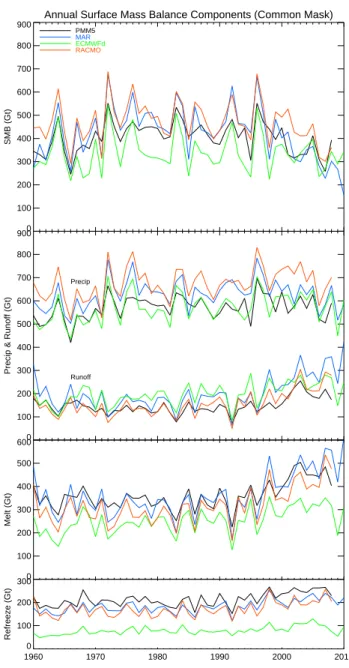
1960 1970 1980 1990 2000 2010 0 100 200 300 Refreeze (Gt) 0 100 200 300 400 500 600 Melt (Gt) 0 100 200 300 400 500 600 700 800 900

Precip & Runoff (Gt)

Precip

Runoff

Annual Surface Mass Balance Components (Common Mask)

0 100 200 300 400 500 600 700 800 900 SMB (Gt) PMM5 MAR ECMWFd RACMO

Fig. 4. Time series of SMB and components on the common mask.

integrated estimate. Since there is less agreement between the models’ representation of the ablation processes (melt, refreeze, runoff), reducing this area while maintaining the ac-cumulation area decreases the variability between the mod-els. The mask used for ECMWFd estimates is the smallest and therefore the closest to the common mask (Table 1) yet RACMO and MAR are the least affected by the change. This highlights the disproportionate impact of some regions of permanent ice cover.

3.2 SMB components

Annual time series of total SMB and SMB components (pre-cipitation, runoff, melt and refreeze) for the common mask are presented in Fig. 4. There is large inter-annual variability

(8)

Table 3. Annual regional SMB (common mask); the mean over 1961–1990 period and the change over 1996–2008 period. Largest change highlighted in bold.

Region ECMWFd RACMO MAR PMM5 ECMWFd RACMO MAR PMM5 1961–1990 1961–1990 1961–1990 1961–1990 1996–2008 1996–2008 1996–2008 1996–2008 [Gt yr−1] [Gt yr−1] [Gt yr−1] [Gt yr−1] Change Change Change Change

Total 341 479 450 413 A 15.8 19.3 20.9 7.2 −82.6 % −101.3 % −142.7 % −180.4 % B 28.3 24.9 52.6 46.2 −12.1 % −77.0 % −36.5 % −40.7 % C 56.2 68.0 83.0 67.5 6.2 % −3.1 % −11.7 % −13.2 % D 96.9 177 133 123 −9.0 % −23.9 % −36.8 % −26.7 % E 103 109 102 112 −31.1 % −61.6 % −76.5 % −33.5 % F 41.1 81.5 57.7 56.4 −80.2 % −54.2 % −86.4 % −60.5 %

with the standard deviation of SMB (PMM5 70 Gt, MAR 106 Gt, ECMWFd 83 Gt and RACMO 91 Gt) being 17 %, 25 %, 24 % and 19 % of the respective mean SMB estima-tions. This variability may provide a partial explanation for the disagreements (Alley et al., 2010) in mass balance esti-mation based on observation (altimetry and gravimetry) over the last decade as studies are typically carried out over differ-ent periods. Relatively small differences in the study period can have significant impact on the period’s mean. There is reasonable correlation (SMB r value = 0.75–0.91, precipita-tion = 0.75–0.93, runoff = 0.73–0.95, melt = 0.84–0.96, re-freeze = 0.69–0.88) between the four models’ annual time series which is unsurprising due to the constraint provided by the common ERA-40 forcing. As indicated by the inter-model spread (Fig. 3), however, large variations in the abso-lute values remain, especially for refreeze.

The GrIS has undergone a climate forcing with surface air temperatures increasing over the study period (Box et al., 2011; Hanna et al., 2008). While the impact of this is evi-dent in the annual time series, the models’ sensitivity to forc-ing since the mid-1990s is more apparent when viewed as a cumulative anomaly from a reference period. This approach also minimises the effects of biases present in the models. The period 1961–1990 has been used in a number of previ-ous studies to represent a climatological mean when the ice sheet was close to balance (Hanna et al., 2005; Rignot et al., 2008) and we use the same approach for estimating anoma-lies.

Each model’s cumulative anomaly for SMB, precipitation and runoff is plotted in Fig. 5. These cumulative anomalies are important when used in mass budget estimates as dif-ferences in cumulative anomaly translate directly into differ-ences in the mass imbalance calculated. Thus, using MAR would result in mass imbalance (from 2000–2010) that is about 1000 Gt larger than for ECMWFd and 500 Gt larger than for RACMO and PMM5. In other words the trend is about 100 Gt a−1 larger for MAR than ECMWFd due to a greater sensitivity in runoff during this period in MAR. The runoff increase over the 2000s results from the ablation area expansion as observed by the MODIS satellite product (Box

et al., 2012). The current runoff increase is higher in MAR because this model uses a fixed bare ice albedo of 0.45, which is lower than other models. This results in larger bare ice areas, which have a greater impact on the MAR melt. On the other hand, the current bare ice area expansion could be overestimated in MAR although it compares well with the MODIS-based estimations (Tedesco et al., 2012). It is impor-tant to remember here that the four models are all respond-ing to the same external forcrespond-ing, yet their SMB sensitivity is markedly different.

The 1995–2008 SMB decrease in RACMO, MAR and PMM5 is comparable in magnitude to the change from 1960–1972. However, the earlier change appears to have re-sulted solely from a decrease in precipitation during a period when runoff for each reconstruction was stable. The SMB decrease is correlated with a decrease in precipitation. The recent decline by contrast is associated with increased pre-cipitation and an even greater increase in runoff. This strik-ing difference in recent behaviour compared with the previ-ous period of reduced SMB demonstrates the importance of accurate modelling of runoff and its most significant compo-nents: melt and refreeze.

The magnitude of the SMB response from each model is different during this recent period (1995–2008) compared with the earlier period (1960–1972). There is greater agree-ment between the precipitation estimates than runoff mates. The sensitivity of RACMO and MAR runoff esti-mates to the same re-analysis forcing is twice and three times, respectively, that of the similar PMM5 and ECMWFd. Since the mid-1990s the GrIS SMB, while remaining posi-tive, shows a negative anomaly (Fig. 5). This decrease is dif-ferent from a similar decrease seen in the period 1960–1972 in that it occurs during a period of increased precipitation where the earlier decline was driven by low precipitation. The recent decline in SMB is due to an increase in runoff.

3.3 Equilibrium line altitude

The area above the ELA, the accumulation area, is inde-pendent of mask differences but captures the net behaviour

(9)

Table 4. Annual regional runoff (common mask); the mean over 1961–1990 period and the change over 1996–2008 period. Largest change highlighted in bold.

Region ECMWFd RACMO MAR PMM5 ECMWFd RACMO MAR PMM5 1961–1990 1961–1990 1961–1990 1961–1990 1996–2008 1996–2008 1996–2008 1996–2008 [Gt yr−1] [Gt yr−1] [Gt yr−1] [Gt yr−1] Change Change Change Change

Total 180 133 168 135 A 17.1 10.2 11.3 22.1 66.8 % 141.0 % 131.2 % 78.1 % B 29.7 18.1 8.5 15.4 36.5 % 85.0 % 103.1 % 63.9 % C 6.9 5.5 3.9 1.4 87.9 % 67.3 % 96.0 % 153.7 % D 23.9 23.4 33.8 19.5 −2.9 % 31.3 % 43.1 % 50.3 % E 64.3 65.9 82.5 54.8 17.2 % 88.9 % 78.0 % 17.1 % F 38.3 10.2 28.2 21.6 122.4 % 453.8 % 147.8 % 96.0 %

RACMO Cumulative Anomaly

1960 1970 1980 1990 2000 2010 −1000 −500 0 500 1000 1500

Cumulative Mass Anomaly (Gt)

MAR Cumulative Anomaly

1960 1970 1980 1990 2000 2010 −1000 −500 0 500 1000 1500

PMM5 Cumulative Anomaly 1960 1970 1980 1990 2000 2010 −1000 −500 0 500 1000 1500

ECMWFd Cumulative Anomaly

1960 1970 1980 1990 2000 2010 −1000 −500 0 500 1000 1500

Surface Mass Balance Precipitation Runoff

Fig. 5. SMB, precipitation and runoff cumulative anomalies from the 1961–1990 period for each model.

of accumulation processes. Above the ELA there is net ac-cumulation. Below the ELA, net ablation prevails. During the 1961–1990 period, the modelled ELA and hence the area above the ELA was approximately stable in each of the four models and averaged: PMM5 1.49 × 106 km2, MAR 1.52 × 106 km2, ECMWFd 1.48 × 106 km2 and RACMO 1.53 × 106 km2. Since the mid-1990s, however, PMM5, MAR and RACMO have a rising ELA and shrinking ac-cumulation area at a rate of approximately 60 000 km2 per decade. ECMWFd, also with the lowest melt and associated lowest refreeze, does not show a significant difference

be-tween the two periods. The rise of the ELA is not due to decreased precipitation; precipitation has increased over this period. It is due to increased runoff, as a result of increased melt outweighing this increased precipitation (Mote, 2007). For MAR and RACMO this increased runoff is due to expan-sion of bare ice areas which significantly deceases the albedo (Tedesco et al., 2011). The satellite derived albedo product used by PMM5 should also capture this decrease. ECMWFd does not model or incorporate albedo variations.

(10)

A

B

C

D

E

F

500 km

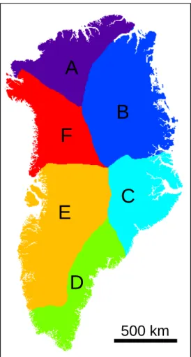
Fig. 6. The Greenland ice sheet is divided into six regions (A–F) based on groupings of drainage basins identified by Rignot et al. (2008).

3.4 Regional analysis

To examine the regional variations between the models, Greenland is divided into six regions (Fig. 6) based on group-ings of drainage basins identified in Rignot et al. (2008). For each region two comparisons are made for SMB and runoff; first the average annual SMB (Fig. 7) and runoff (Fig. 8) dur-ing the 1961–1990 reference period and secondly the rate of change during the 1996–2008 period. Data for SMB and runoff are provided in Table 3 and Table 4, respectively. The first observation to note is that the rank order of the models varies from region to region. RACMO has the highest SMB in regions D and F, yet the lowest in region B. PMM5 esti-mates the highest SMB in region E, yet the lowest in A. Rank order also varies for runoff. MAR has lowest runoff in region B, yet the highest in D and E and PMM5 has the highest runoff in region A, yet lowest in C.

In four out of six regions (A, B, D and F), the high-est model’s SMB high-estimate is approximately double the low-est, a much larger inter-model difference than seen over the whole ice sheet (Fig. 3). ECMWFd usually shows the

small-Table 5. Difference between modelled and observed SMB above 1500 m.

Model RMS Error RMS Error [mm w.e. yr−1] [percent of obs. mean]

RACMO 76 21 %

MAR 172 46 %

PMM5 67 18 %

ECMWFd 62 17 %

Table 6. Difference between modelled and observed SMB below 1500 m (K-transect).

Model RMS Error RMS Error [mm w.e. yr−1] [percent of obs. mean]

RACMO 773 38 %

MAR 489 24 %

PMM5 591 29 %

ECMWFd 1939 95 %

est change in SMB over the 1996–2008 period. This recon-struction is the least sensitive to the common forcing. MAR and PMM5 usually show the largest response. These regional variations suggest spatially compensating errors are leading to the appearance of greater agreement over the whole ice sheet than the localised process modelling is able to repro-duce. They imply that, at a basin scale, the errors in one or more model are significantly (up to a factor 2) larger than at the whole ice sheet scale. This also has important implica-tions for the confidence given to mass budget estimates at a basin scale. Moreover, basins along the southwest and north coast are projected to have the highest sensitivity of SMB to increasing temperatures (Tedesco and Fettweis, 2012).

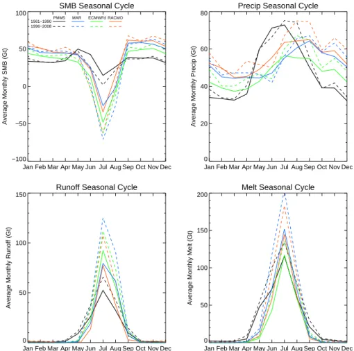
3.5 Seasonal cycle

The seasonal cycle describes each model’s sensitivity to a common seasonal forcing. Figure 9 illustrates the seasonal cycle for SMB and precipitation, runoff and melt compo-nents over both the 1961–1990 and 1996–2008 periods. For the 1961–1990 period, monthly SMB is generally positive, adding between 30 and 60 Gt to the ice sheet except for the peak melt period (June–August) where, despite increased precipitation, there is a net mass loss due to runoff. PMM5 appears to be an outlier with a smaller SMB seasonal cy-cle and including an increase in SMB in May caused by an earlier increase in precipitation than the other models. The precipitation seasonal cycle is greater in magnitude and ear-lier by several months. PMM5’s runoff seasonal cycle is a little over half the magnitude of the other models. This is likely to be due to the PMM5 snow model not being fully coupled to the atmosphere so neither melt-albedo feedback, nor expansion of dark, bare ice is explicitly considered. This

(11)

0 5 10 15 20 SMB Gt/yr

ECMWFd RACMO MAR PMM5

0 10 20 30 40 50 SMB Gt/yr

0 20 40 60 80 SMB Gt/yr

0 50 100 150

SMB Gt/yr

0 20 40 60 80 100 SMB Gt/yr

0 20 40 60 80 SMB Gt/yr

A B C

D E F

Fig. 7. Average annual SMB [Gt yr−1] for six regions for the 1961–1990 period.

0 5 10 15 20 Runoff Gt/yr

0 5 10 15 20 25 Runoff Gt/yr

0 1 2 3 4 5 6 Runoff Gt/yr

0 5 10 15 20 25 30 Runoff Gt/yr

0 20 40 60 80 Runoff Gt/yr

0 10 20 30

Runoff Gt/yr

A B C

D E F

Fig. 8. Average annual runoff [Gt yr−1] for six regions for the 1961–1990 period.

period includes the dip and recovery in SMB between 1960 and 1980 due to changes in precipitation. However, this is not expected to affect the mean SMB or precipitation sea-sonal cycles.

During the 1996–2008 period each model estimates slightly increased SMB during the non-summer months of positive SMB with respect to the 1961–1990 period. This is due to increased precipitation, however, this increase is out-weighed by reduced SMB during the summer months due to increased melt driven runoff. The magnitude of the response in this latter period does vary significantly between models. For the three months, JJA, total melt increased by: MAR

43 %, RACMO 38 %, ECMWFd 28 %, and PMM5 27 %. The two models with fully coupled snow models (RACMO and MAR) show the larger melt response, most probably because they allow for feedbacks between the atmosphere and sur-face. This highlights the limitation of not considering the melt-albedo feedback in a coupled approach.

3.6 Comparison with observation

Figure 10 compares in situ SMB observation with equivalent (location, period) modelled SMB estimates. Model estimates differ from observations by a larger amount in the ablation

(12)

SMB Seasonal Cycle

Jan Feb Mar Apr May Jun Jul Aug Sep Oct Nov Dec −100 −50 0 50 100 Average Monthly SMB (Gt) 1961−1990 1996−2008

PMM5 MAR ECMWFd RACMO

Precip Seasonal Cycle

Jan Feb Mar Apr May Jun Jul Aug Sep Oct Nov Dec 0

20 40 60 80

Average Monthly Precip (Gt)

Runoff Seasonal Cycle

50 100 150

Average Monthly Runoff (Gt)

Melt Seasonal Cycle

50 100 150 200

Average Monthly Melt (Gt)

Fig. 9. Seasonal cycle of SMB, precipitation, runoff and melt for each model averaged over the 1961–1990 and 1996–2008 periods.

In situ obs. and modelled SMB (K−transect)

0 1 2 3 4 In situ rank order −6 −5 −4 −3 −2 −1 0 SMB (m w.e. yr −1)

In situ obs. and modelled SMB above 1500 m

0 20 40 60 80 100 In situ rank order

0.0 0.2 0.4 0.6 0.8 1.0 SMB (m w.e. yr −1) Observation PMM5 MAR ECMWFd RACMO

Fig. 10. In situ SMB observations (purple) plotted in increasing SMB (rank) order along horizontal axis with the equivalent model estimated SMB in colour.

(13)

area (Table 6) than the accumulation area (Table 5). It should be noted that both ECMWFd and PMM5 have used in situ observations during their calibration. Those data have not been separated out from other observations so the compar-ison shown here is not fully independent for those two mod-els. We would expect this to result in ECMWFd and PMM5 showing lower RMS errors than RACMO and MAR in the accumulation area.

In the accumulation area, MAR tends to overestimate SMB. In comparison to RACMO, this overestimation is due to increased precipitation in the interior of the ice sheet, lead-ing to fewer bare ice pixels and higher albedo (Fettweis et al., 2011). ECMWFd significantly overestimates ablation along the low elevation K-transect due to higher melt driven runoff in this area.

4 Conclusions

The same climate reanalysis data have been used to force four different models in order to estimate Greenland ice sheet surface mass balance and its sub-components. First, we con-sidered the effect of the ice sheet mask. Total surface mass balance estimates from the four models for the ice sheet show reasonable agreement once mapped onto the common mask. Applying the common mask to model output decreases the variation between models. However, part of this reduction may only be a result of reducing the amount of ablation area, where disagreement is larger, but leaving the accumulation area the same size. The largest inter-model variations remain for refreeze estimates. ECMWFd’s refreeze estimate deviates most from the other three models and therefore contributes most to the observed inter-model variation. ECMWFd’s low refreeze is partially attributable to its lower melt magnitude but the main difference with respect to the other models is the use of a degree-day approach instead of an energy bal-ance model. Modelled surface mass balbal-ance uncertainty may be smaller than previously thought due to variations in the native mask, and so we recommend the use of an accurate common mask for future modelling work.

The differences between models both at the whole ice sheet (native masks), and more acutely at the basin scale, are larger than the combined RMS errors of the models, suggest-ing an underestimation of the model error. This has implica-tions for uncertainty estimates in mass balance studies based on the mass budget or input-output method.

Next, we compared the physical differences between the models by component and by region now on the common mask. There are large regional inter-model variations, and, in particular, the rank order of the model outputs vary consid-erably regionally, suggesting a likely spatial compensation of errors. This compensation exaggerates the level of agree-ment seen over the whole ice sheet leading to the appearance of greater agreement than the localised process modelling is able to reproduce. The variations in ice sheet mask increased

apparent differences in the modelled estimates, which can be partly alleviated by using a common mask. More work is needed to understand the origin of the regional differ-ences between models as, whilst the current differdiffer-ences re-duce when integrated over the whole ice sheet, this may not continue to be the case as the climate over the GrIS changes in the future.

The comparison of SMB components revealed a change in the physical drivers of ice sheet reduction. The decreas-ing annual SMB modelled since the mid-1990s is similar to the earlier period 1960–1972, however, where the earlier de-crease is due to reduced precipitation with runoff remaining unchanged, the recent decrease is associated with increased precipitation, now more than compensated for by increased melt driven runoff. The ability to separate the components of SMB in this way is a strength of the modelling approach used here. We examined the response of the four models to the common forcing since the 1990s and also to the seasonal cycle and found marked differences between the models in terms of cumulative SMB anomaly and amplitude of sea-sonal cycle, with differences of up to factor 3 and 2, respec-tively.

Finally a comparison was made with in situ observation data. ECMWFd and PMM5 have used some in situ data dur-ing their development which is likely to explain the lower RMS errors seen in the accumulation area for these recon-structions. Modelled estimates differ from observations by a larger amount in the ablation area, suggesting melt and re-freeze, with their strong albedo feedbacks, are more chal-lenging to model than the precipitation downscaling .

Future work should focus on the physical reasons for the regional differences identified here, in order to inform future model development. The models investigated in this study are continuously under development and comparisons between simulations with new and improved physics are likely to reduce or ameliorate the discrepancies that we identified in this analysis.

Acknowledgements. We thank the editor and the two anonymous

reviewers for their constructive comments, which have greatly improved this manuscript. Funding for this study was provided by a NERC studentship awarded to C. L. Vernon.

Edited by: G. H. Gudmundsson

References

Alley, R. B., Andrews, J. T., Brigham-Grette, J., Clarke, G. K. C., Cuffey, K. M., Fitzpatrick, J. J., Funder, S., Marshall, S. J., Miller, G. H., Mitrovica, J. X., Muhs, D. R., Otto-Bliesner, B. L., Polyak, L., and White, J. W. C.: History of the Greenland Ice Sheet: paleoclimatic insights, Quaternary. Sci. Rev., 29, 1728– 1756, doi:10.1016/j.quascirev.2010.02.007, 2010.

(14)

Bales, R. C., McConnell, J. R., Mosley-Thompson, E., and Csatho, B.: Accumulation over the Greenland ice sheet from historical and recent records, J. Geophys. Res.-Atmos., 106, 33813–33825, 2001.

Bales, R. C., Guo, Q. H., Shen, D. Y., McConnell, J. R., Du, G. M., Burkhart, J. F., Spikes, V. B., Hanna, E., and Cappelen, J.: Annual accumulation for Greenland updated using ice core data developed during 2000-2006 and analysis of daily coastal meteorological data, J. Geophys. Res.-Atmos., 114, D06116, doi:10.1029/2008jd011208, 2009.

Bougamont, M., Bamber, J. L., and Greuell, W.: A surface mass bal-ance model for the Greenland ice sheet, J. Geophys. Res.-Earth, 110, F04018, doi:10.1029/2005JF000348, 2005.

Box, J. E., Bromwich, D. H., and Bai, L. S.: Greenland ice sheet surface mass balance 1991–2000: Application of Polar MM5 mesoscale model and in situ data, J. Geophys. Res.-Atmos., 109, D16105, doi:10.1029/2003jd004451, 2004.

Box, J. E., Bromwich, D. H., Veenhuis, B. A., Bai, L. S., Stroeve, J. C., Rogers, J. C., Steffen, K., Haran, T., and Wang, S. H.: Green-land ice sheet surface mass balance variability (1988–2004) from calibrated polar MM5 output, J. Climate, 19, 2783–2800, 2006. Box, J. E., Yang, L., Bromwich, D. H., and Bai, L. S.: Greenland Ice

Sheet Surface Air Temperature Variability: 1840–2007, J. Cli-mate, 22, 4029–4049, 10.1175/2009jcli2816.1, 2009.

Box, J. E., Cappelen, J., Chen, C., Decker, D., Fettweis, X., Hall, D., Hanna, E., Jorgensen, B. V., Knudsen, N. T., Lipscomb, W. H., Mernild, S. H., Mote, T., Steiner, N., Tedesco , M., van de Wal, R. S. W., and Wahr, J.: Greenland Ice Sheet, Arctic Report Card: Update for 2011, available at: http://www.arctic.noaa.gov/ reportcard/greenland_ice_sheet.html, 2011.

Box, J. E., Fettweis, X., Stroeve, J. C., Tedesco, M., Hall, D. K., and Steffen, K.: Greenland ice sheet albedo feedback: thermo-dynamics and atmospheric drivers, The Cryosphere, 6, 821–839, doi:10.5194/tc-6-821-2012, 2012.

Brun, E., David, P., Sudul, M., and Brunot, G.: A numerical model to simulate snow-cover stratigraphy for operational avalanche forecasting, J. Glaciol., 38, 13–22, 1992.

Cogley, J. G.: Greenland accumulation: An error model, J. Geophys. Res.-Atmos., 109, D18101, doi:10.1029/2003jd004449, 2004. Dahl-Jensen, D., Bamber, J., Bøggild,C. E., Buch, E., Christensen,

J. H., Dethloff, K., Fahnestock, M., Marshall, S., Rosing, M., Steffen, K., Thomas, R., Truffer, M., van den Broeke, M., and Veen, C. J. v. d.: The Greenland Ice Sheet in a Changing Climate: Snow, Water, Ice and Permafrost in the Arctic (SWIPA), Arctic Monitoring and Assessment Programme (AMAP), Oslo, 115 pp., 2009.

De Ridder, K. and Gallee, H.: Land surface-induced regional cli-mate change in southern Israel, J. Appl. Meteorol., 37, 1470– 1485, 1998.

Dee, D. P., Uppala, S. M., Simmons, A. J., Berrisford, P., Poli, P., Kobayashi, S., Andrae, U., Balmaseda, M. A., Balsamo, G., Bauer, P., Bechtold, P., Beljaars, A. C. M., van de Berg, L., Bid-lot, J., Bormann, N., Delsol, C., Dragani, R., Fuentes, M., Geer, A. J., Haimberger, L., Healy, S. B., Hersbach, H., Hólm, E. V., Isaksen, L., Kållberg, P., Köhler, M., Matricardi, M., McNally, A. P., Monge-Sanz, B. M., Morcrette, J. J., Park, B. K., Peubey, C., de Rosnay, P., Tavolato, C., Thépaut, J. N., and Vitart, F.: The ERA-Interim reanalysis: configuration and performance of the data assimilation system, Q. J. Roy. Meteorol. Soc., 137, 553–

597, doi:10.1002/qj.828, 2011.

Ettema, J., van den Broeke, M. R., van Meijgaard, E., van de Berg, W. J., Bamber, J. L., Box, J. E., and Bales, R. C.: Higher sur-face mass balance of the Greenland ice sheet revealed by high-resolution climate modeling, Geophys. Res. Lett., 36, L12501, doi:10.1029/2009gl038110, 2009.

Ettema, J., van den Broeke, M. R., van Meijgaard, E., and van de Berg, W. J.: Climate of the Greenland ice sheet using a high-resolution climate model – Part 2: Near-surface climate and en-ergy balance, The Cryosphere, 4, 529–544, doi:10.5194/tc-4-529-2010, 2010a.

Ettema, J., van den Broeke, M. R., van Meijgaard, E., van de Berg, W. J., Box, J. E., and Steffen, K.: Climate of the Greenland ice sheet using a high-resolution climate model – Part 1: Evaluation, The Cryosphere, 4, 511–527, doi:10.5194/tc-4-511-2010, 2010b. Fettweis, X.: Reconstruction of the 1979–2006 Greenland ice sheet surface mass balance using the regional climate model MAR, The Cryosphere, 1, 21–40, doi:10.5194/tc-1-21-2007, 2007. Fettweis, X., Gallee, H., Lefebre, F., and van Ypersele, J. P.:

Green-land surface mass balance simulated by a regional climate model and comparison with satellite-derived data in 1990–1991, Clim. Dynam., 24, 623–640, doi:10.1007/s00382-005-0010-y, 2005. Fettweis, X., Hanna, E., Gallée, H., Huybrechts, P., and Erpicum,

M.: Estimation of the Greenland ice sheet surface mass balance for the 20th and 21st centuries, The Cryosphere, 2, 117–129, doi:10.5194/tc-2-117-2008, 2008.

Fettweis, X., Tedesco, M., van den Broeke, M., and Ettema, J.: Melting trends over the Greenland ice sheet (1958–2009) from spaceborne microwave data and regional climate models, The Cryosphere, 5, 359–375, doi:10.5194/tc-5-359-2011, 2011. Franco, B., Fettweis, X., Lang, C., and Erpicum, M.: Impact of

spa-tial resolution on the modelling of the Greenland ice sheet sur-face mass balance between 1990–2010, using the regional cli-mate model MAR, The Cryosphere, 6, 695–711, doi:10.5194/tc-6-695-2012, 2012.

Gallée, H. and Schayes, G.: Development of a Three-Dimensional Meso-γ Primitive Equation Model: Katabatic Winds Simulation in the Area of Terra Nova Bay, Antarctica, Mon. Weather Rev., 122, 671–685., 1994.

Gregory, J. M. and Huybrechts, P.: Ice-sheet contributions to future sea-level change, Philos. T. R. Soc. A, 364, 1709–1731, 2006. Greuell, W. and Konzelmann, T.: Numerical Modeling of the

Energy-Balance and the Englacial Temperature of the Green-land Ice-Sheet - Calculations for the Eth-Camp Location (West Greenland, 1155m Asl), Global Planet. Change, 9, 91–114, 1994. Hall, D. K., Riggs, G. A., and Salomonson, V. V.: MODIS/Terra Snow Cover Daily L3 Global 500 m Grid V004, January to March 2003, Digital media, updated daily, National Snow and Ice Data Center, Boulder, CO, USA, 2011.

Hanna, E., Huybrechts, P., and Mote, T. L.: Surface mass balance of the Greenland ice sheet from climate-analysis data and accumu-lation/runoff models, Ann. Glaciol., 35, 35, 67–72, 2002. Hanna, E., Huybrechts, P., Janssens, I., Cappelen, J., Steffen, K.,

and Stephens, A.: Runoff and mass balance of the Greenland ice sheet: 1958–2003, J. Geophys. Res.-Atmos., 110, D13108, doi:10.1029/2004JD005641, 2005.

Hanna, E., Huybrechts, P., Steffen, K., Cappelen, J., Huff, R., Shuman, C., Irvine-Fynn, T., Wise, S., and Griffiths, M.: Increased runoff from melt from the Greenland Ice Sheet:

(15)

A response to global warming, J. Climate, 21, 331–341, doi:10.1175/2007jcli1964.1, 2008.

Hanna, E., Huybrechts, P., Cappelen, J., Steffen, K., Bales, R. C., Burgess, E., McConnell, J. R., Steffensen, J. P., Van den Broeke, M., Wake, L., Bigg, G., Griffiths, M., and Savas, D.: Greenland Ice Sheet surface mass balance 1870 to 2010 based on Twentieth Century Reanalysis, and links with global climate forcing, J. Geophys. Res.-Atmos., 116, D24121, doi:10.1029/2011jd016387, 2011.

Huybrechts, P., Gregory, J., Janssens, I., and Wild, M.: Modelling Antarctic and Greenland volume changes dur-ing the 20th and 21st centuries forced by GCM time slice integrations, Global Planet. Change, 42, 83–105, doi:10.1016/j.gloplacha.2003.11.011, 2004.

Huybrechts, P., Goelzer, H., Janssens, I., Driesschaert, E., Fichefet, T., Goosse, H., and Loutre, M. F.: Response of the Greenland and Antarctic Ice Sheets to Multi-Millennial Greenhouse Warming in the Earth System Model of Intermediate Complexity LOVE-CLIM, Surv. Geophys., 32, 397–416, doi:10.1007/s10712-011-9131-5, 2011.

Janssens, I. and Huybrechts, P.: The treatment of meltwater re-tention in mass-balance parameterizations of the Greenland ice sheet, in: Ann. Glaciol., 31, 2000, edited by: Steffen, K., Ann. Glaciol., Int Glaciological Soc, Cambridge, 133–140, 2000. Kargel, J. S., Ahlstrøm, A. P., Alley, R. B., Bamber, J. L., Benham,

T. J., Box, J. E., Chen, C., Christoffersen, P., Citterio, M., Cogley, J. G., Jiskoot, H., Leonard, G. J., Morin, P., Scambos, T., Shel-don, T., and Willis, I.: Brief communication Greenland’s shrink-ing ice cover: “fast times” but not that fast, The Cryosphere, 6, 533–537, doi:10.5194/tc-6-533-2012, 2012.

Key, J., Fowler, C., Maslanik, J., Haran, T., Scambos, T., and Emery, W.: The Extended AVHRR Polar Pathfinder (APP-x) Product, v 1.0. Digital Media, Space Science and Engineering Center, Uni-versity of Wisconsin, Madison, WI., 2006.

Lefebre, F., Gallee, H., van Ypersele, J. P., and Greuell, W.: Mod-eling of snow and ice melt at ETH Camp (West Greenland): A study of surface albedo, J. Geophys. Res.-Atmos., 108, 4231, doi:10.1029/2001jd001160, 2003.

Lucas-Picher, P., Wulff-Nielsen, M., Christensen, J. H., Aðal-geirsdóttir, G., Mottram, R., and Simonsen, S. B.: Very high resolution regional climate model simulations over Green-land: Identifying added value, J. Geophys. Res., 117, D02108, doi:10.1029/2011jd016267, 2012.

Mernild, S. H. and Liston, G. E.: Greenland freshwater runoff. Part II: Distribution and trends, 1960–2010, J. Climate, 6015–6035, doi:10.1175/jcli-d-11-00592.1, 2012.

Mote, T. L.: Greenland surface melt trends 1973–2007: Evidence of a large increase in 2007, Geophys. Res. Lett., 34, L22507, doi:10.1029/2007gl031976, 2007.

Overland, J. E., Wang, M. Y., Bond, N. A., Walsh, J. E., Kattsov, V. M., and Chapman, W. L.: Considerations in the Selec-tion of Global Climate Models for Regional Climate Projec-tions: The Arctic as a Case Study, J. Climate, 24, 1583–1597, doi:10.1175/2010jcli3462.1, 2011.

Pfeffer, W. T., Meier, M. F., and Illangasekare, T. H.: Retention of Greenland runoff by refreezing – implications for projected future sea-level change, J. Geophys. Res.-Oceans, 96, 22117– 22124, doi:10.1029/91jc02502, 1991.

Rae, J. G. L., Aðalgeirsdóttir, G., Edwards, T. L., Fettweis, X., Gre-gory, J. M., Hewitt, H. T., Lowe, J. A., Lucas-Picher, P., Mottram, R. H., Payne, A. J., Ridley, J. K., Shannon, S. R., van de Berg, W. J., van de Wal, R. S. W., and van den Broeke, M. R.: Greenland ice sheet surface mass balance: evaluating simulations and mak-ing projections with regional climate models, The Cryosphere, 6, 1275–1294, doi:10.5194/tc-6-1275-2012, 2012.

Reijmer, C. H., van den Broeke, M. R., Fettweis, X., Ettema, J., and Stap, L. B.: Refreezing on the Greenland ice sheet: a comparison of parameterizations, The Cryosphere, 6, 743–762, doi:10.5194/tc-6-743-2012, 2012.

Rignot, E., Box, J. E., Burgess, E., and Hanna, E.: Mass balance of the Greenland ice sheet from 1958 to 2007, Geophys. Res. Lett., 35, L20502, doi:10.1029/2008gl035417, 2008.

Rignot, E., Velicogna, I., van den Broeke, M. R., Monaghan, A., and Lenaerts, J.: Acceleration of the contribution of the Greenland and Antarctic ice sheets to sea level rise, Geophys. Res. Lett., 38, L05503, doi:10.1029/2011gl046583, 2011.

Sasgen, I., van den Broeke, M., Bamber, J. L., Rignot, E., Sorensen, L. S., Wouters, B., Martinec, Z., Velicogna, I., and Simonsen, S. B.: Timing and origin of recent regional ice-mass loss in Greenland, Earth Planet. Sci. Lett., 333, 293–303, doi:10.1016/j.epsl.2012.03.033, 2012.

Steffen, K. and Box, J.: Surface climatology of the Greenland ice sheet: Greenland climate network 1995–1999, J. Geophys. Res.-Atmos., 106, 33951–33964, 2001.

Stephenson, D. B., Collins, M., Rougier, J. C., and Chandler, R. E.: Statistical problems in the probabilistic prediction of climate change, Environmetrics, 23, 364–372, doi:10.1002/env.2153, 2012.

Stroeve, J. C., Box, J. E., and Haran, T.: Evaluation of the MODIS (MOD10A1) daily snow albedo product over the Greenland ice sheet, Remote Sens. Environ., 105, 155–171, doi:10.1016/j.rse.2006.06.009, 2006.

Tedesco, M. and Fettweis, X.: 21st century projections of surface mass balance changes for major drainage systems of the Green-land ice sheet, Environ. Res. Lett., 7, 045405, doi:10.1088/1748-9326/7/4/045405, 2012.

Tedesco, M., Fettweis, X., van den Broeke, M. R., van de Wal, R. S. W., Smeets, C., van de Berg, W. J., Serreze, M. C., and Box, J. E.: The role of albedo and accumulation in the 2010 melting record in Greenland, Environ. Res. Lett., 6, 014005, doi:10.1088/1748-9326/6/1/014005, 2011.

Tedesco, M., Fettweis, X., Mote, T., Wahr, J., Alexander, P., Box, J., and Wouters, B.: Evidence and analysis of 2012 Greenland records from spaceborne observations, a regional climate model and reanalysis data, The Cryosphere Discuss., 6, 4939–4976, doi:10.5194/tcd-6-4939-2012, 2012.

Uppala, S. M., Kallberg, P. W., Simmons, A. J., Andrae, U., Bech-told, V. D., Fiorino, M., Gibson, J. K., Haseler, J., Hernandez, A., Kelly, G. A., Li, X., Onogi, K., Saarinen, S., Sokka, N., Al-lan, R. P., Andersson, E., Arpe, K., Balmaseda, M. A., Beljaars, A. C. M., Van De Berg, L., Bidlot, J., Bormann, N., Caires, S., Chevallier, F., Dethof, A., Dragosavac, M., Fisher, M., Fuentes, M., Hagemann, S., Holm, E., Hoskins, B. J., Isaksen, L., Janssen, P., Jenne, R., Mcnally, A. P., Mahfouf, J. F., Morcrette, J. J., Rayner, N. A., Saunders, R. W., Simon, P., Sterl, A., Trenberth, K. E., Untch, A., Vasiljevic, D., Viterbo, P., and Woollen, J.: The ERA-40 re-analysis. Q. J. Roy. Meteor. Soc., 131, 2961–3012,

(16)

2005.

van de Wal, R. S. W., Boot, W., Smeets, C. J. P. P., Snellen, H., van den Broeke, M. R., and Oerlemans, J.: Twenty-one years of mass balance observations along the K-transect, West Green-land, Earth Syst. Sci. Data, 4, 31–35, doi:10.5194/essd-4-31-2012, 2012.

van den Broeke, M., Bamber, J., Ettema, J., Rignot, E., Schrama, E., van de Berg, W. J., van Meijgaard, E., Velicogna, I., and Wouters, B.: Partitioning Recent Greenland Mass Loss, Science, 326, 984– 986, doi:10.1126/science.1178176, 2009.

van Meijgarrd, E., van Ulft, L. H., Van De Berg, W. J., Bosveld, F. C., Van den Hurk, B. J. J. M., Lenderink, G., and Siebesma, A. P.: The KNMI regional atmospheric climate model RACMO version 2.1, KNNI, PO Box 201, 3730 AE De Bilt, Wilhelminalaan 10, De Bilt, the Netherlands, 2008.

Velicogna, I.: Increasing rates of ice mass loss from the Green-land and Antarctic ice sheets revealed by GRACE, Geophys. Res. Lett., 36, L19503, doi:10.1029/2009gl040222, 2009.