HAL Id: hal-01879628
https://hal.archives-ouvertes.fr/hal-01879628v2
Submitted on 18 Oct 2018
HAL is a multi-disciplinary open access
archive for the deposit and dissemination of
sci-entific research documents, whether they are
pub-lished or not. The documents may come from
teaching and research institutions in France or
abroad, or from public or private research centers.
L’archive ouverte pluridisciplinaire HAL, est
destinée au dépôt et à la diffusion de documents
scientifiques de niveau recherche, publiés ou non,
émanant des établissements d’enseignement et de
recherche français ou étrangers, des laboratoires
publics ou privés.
CASSIS: Characterization with Adaptive Sample-Size
Inferential Statistics Applied to Inexact Circuits
Justine Bonnot, Vincent Camus, Karol Desnos, Daniel Menard
To cite this version:
Justine Bonnot, Vincent Camus, Karol Desnos, Daniel Menard. CASSIS: Characterization with
Adap-tive Sample-Size Inferential Statistics Applied to Inexact Circuits. EUSIPCO: EUropean SIgnal
Pro-cessing Conference, Sep 2018, Rome, Italy. �10.23919/eusipco.2018.8553451�. �hal-01879628v2�
C
ASSIS
: Characterization with Adaptive
Sample-Size Inferential Statistics Applied to Inexact Circuits
Justine Bonnot
†, Vincent Camus
‡, Karol Desnos
†, Daniel Menard
††Univ. Rennes, INSA Rennes, CNRS, IETR - UMR 6164, F-35000 Rennes, France ‡ICLAB, Ecole Polytechnique F´ed´erale de Lausanne (EPFL), Switzerland
Abstract—To design faster and more energy-efficient systems, numerous inexact arithmetic operators have been proposed, gen-erally obtained by modifying the logic structure of conventional circuits. However, as the quality of service of an application has to be ensured, these operators need to be precisely characterized to be usable in commercial or real-life applications. The characteri-zation of inexact operators is commonly achieved with exhaustive or random bit-accurate gate-level simulations. However, for high word lengths, the time and memory required for such simulations become prohibitive. Besides, when simulating a random sample, no confidence information is given on the precision of the characterization. To overcome these limitations, CASSIS, a new characterization method for inexact operators is proposed. By exploiting statistical properties of the approximation error, the number of simulations needed for precise characterization is drastically reduced. From user-defined confidence requirements, the proposed method computes the minimal number of simu-lations to obtain the desired accuracy on the characterization. For 32-bit adders, the CASSIS method reduces the number of simulations needed up to a few tens of thousands points.
I. INTRODUCTION
Real-time and energy constraints for the current design of embedded systems increase the need for new techniques to save resources during the implementation phase. Approximate Computing is rising as one of the main approaches for post-Moore’s Law computing. It exploits the deliberate introduction or tolerance of errors in order to save energy or accelerate computation speed. The precision of an application is now taken as a new tunable parameter to design more efficient systems.
Approximations in circuits have been introduced in different manners such as overclocking [1] at circuit level or computa-tion skipping [2] at algorithmic level. The logic structure of original exact operators can also be modified into an inexact version [3]–[7]. Inexact operators generate errors with varied amplitude and error rate. The error amplitude depends on the location of the erroneous bits of the operator output. To use an inexact operator in an application, the errors generated by the induced approximations have to be characterized in terms of error rate and amplitude. The impact of the approximation on the application quality metric has to be quantified. The application quality metric, whose measurement depends on the application, quantifies the output quality of the application. For instance, for a signal processing application, the application quality metric can be the SNR. The application designer then computes statistical properties on the error generated
by inexact operators to ensure their behavior in the targeted application and select the most suitable to his constraints.
The error induced by inexact operators can be evaluated with two types of approaches: 1) Analytical methods [8]–[10] mathematically expressing error statistics but the link between these statistics and the impact of the operator on the ap-plication quality metric is not straightforward. 2) Functional simulation techniques [11]–[13] simulate the inexact operator on a representative set of data and computes statistics on the approximation error. This later method is more and more employed due to the increasing amount of data generated in the Cloud or processed by data mining. Nevertheless, to mimic the inexact operator behavior, bit-accurate simulations at the logic-level (BALL simulations) are required to catch the internal structure modifications of the operator. The inexact operator may be simulated exhaustively, i.e. for all the possible inputs, to compute the required statistics, which is not feasible for high word-lengths because of the required simulation time. Commonly, the error statistics are computed by simulating a given number of random inputs. Indeed, BALL simulations are two or three orders of magnitude more complex than classical simulations with native data types. A BALL simulation of a 16-bit inexact adder takes around 300 times more time than a native processor instruction, and even 4000 times longer in the case of an inexact multiplier.
Nevertheless, the quality of the statistical characterization obtained from a random sampling is highly dependent on the number of samples taken and on the chosen input distribution. Besides, the quality of the estimated statistics is not evaluated, and the random sampling based on a fixed number of samples can be ineffective in terms of simulation time. To be used in a real application, a method to characterize inexact operators with a user-defined confidence interval is strongly needed, particularly for high word-length inexact operators.
In this paper, we propose an efficient methodology to characterize inexact operators. The proposed method derives the minimal number of samples to simulate, to characterize an inexact operator given an user-defined confidence infor-mation. Our approach exploits the statistical properties of the approximation error. The number of simulations needed and the characterization time are drastically reduced. Reducing the characterization time allows to characterize high word-lengths operators. This method is demonstrated on several inexact adders of different bitwidths, from 8 to 32 bits, considering both the Mean Error Distance (µe) and Error Rate (f ).
The paper is organized as follows: in Section II, the metrics used for the characterization of inexact operators and the proposed characterization method are presented. Section III presents the simulation time savings offered by the proposed method and the quality of the obtained estimation. Section IV concludes the paper.
II. CHARACTERIZATION WITHADAPTIVESAMPLE-SIZE
INFERENTIALSTATISTICS(CASSIS)
The objectives of the CASSIS method are: 1) to estimate the circuit error characteristics more efficiently, using a reduced but sufficient number of samples, 2) to provide the estimated error characteristics with a given confidence information, which is normally not the case with a fixed amount of samples.
A. Metrics for error characterization of inexact adders Inexact arithmetic circuits are traditionally characterized based on the absolute Error Distance (e) of the calculation output, expressed as:
e = |z − z|b (1)
where bz and z are the erroneous and exact operator outputs, respectively. Then, the Mean Error Distance µeand the error rate f are derived from e, defined as:
µe= 1 N P i ∈ I ei (2) f = P i ∈ I fei N , with fei = ( 1 if ei= 0 0 else (3) where ei is the Error Distance of the ithstimuli on a sample I of size N .
B. Proposed statistical characterization method
Inferential statistics [14] aim at reproducing the behavior of a large population using a subset of this population. Instead of simulating exhaustively all the possible input operands combinations in I, the input operands set is sampled to give an estimation with an accuracy h and a probability p that the estimation is contained within the confidence interval. The CASSIS method computes the minimal number of samples to simulate, to estimate the error characteristics according to (h, p). Nµe and Nf represent the minimal number of samples
to estimate µe and f , respectively. 1) Computation ofNµe
The empirical mean µe, a punctual estimator of µe, i.e. an estimation of µe computed over a given number of samples, is used to estimate µe. µe is used to compute the theoretical number of samples Nµe to simulate to get an estimation ac-cording to the confidence parameters (h, p). To estimate Nµe, the standard deviation of the simulated samples is needed. The empirical mean µe and the empirical standard deviation ˜S2, a biased estimator of the standard deviation σe, are computed over T samples as:
µe= 1 T T X i=1 ei (4) ˜ S2= 1 T T X i=1 (ei− µe)2 (5)
The estimators µe and ˜S2 are associated to confidence intervals ICµe and ICσe respectively, defined such that they
include µe and σe with a probability p. Then, according to the Central Limit Theorem, since (e1, e2, ..., eT) are belong-ing to the same probability set, independent and identically distributed, Equation 6 is verified if the number of samples Nµe is higher than 30. Consequently, no assumption has to be made on the distribution of the population. In Equation 6, N (0, σ) represents a Gaussian distribution whose mean is 0 and standard deviation is σ.
pNµe(µe− µe)
law
−−→ N (0, σ) (6) The confidence interval ICp
µeis developed in Equation 7 and
contains µe with a probability p. The term aα
µe embodies the
accuracy on the estimation and is computed as in Equation 8. zα is given by the table of the standard normal distribution given p. Nµe is the minimal number of samples to simulate to get an estimation respecting the user-defined parameters (h, p).
ICpµe = [µe− aα µe; µe+ a α µe] (7) aαµe = zα· S˜ pNµe− 1 (8) The desired accuracy h on the estimation of the average error distance impacts the number of samples to simulate as expressed in Equation 9. To get a desired accuracy of h, aα
µe
must be lower or equal to h.
Nµe >
z2 α· ˜S2
h2 (9)
According to Equation 9, if the standard deviation of the error generated by the inexact adder is very large, Nµe can be very high. Inexact operators with a large standard deviation renders circuits with poor interest. In the proposed method, a maximal number of simulated points has been fixed to Nmax= 25 · 106. If the required number of points is higher than Nmax, the estimated µe and f are given according to p but with a precision h depending on Nmax.
2) Computation ofNf
The proportion of input operands in I that generates an error is embodied by the error rate f . f follows a hypergeometric law. The estimator used for the error rate is fe, the proportion of samples generating an error in the random sampling. Such an estimator can also be associated to a confidence interval ICpf that is defined such that the real error rate f of the population E is contained in this confidence interval with a probability p. The computation of ICpf is developed in Equation 10.
ICkf = [fe− aα f; fe+ a
α
f] (10) In Equation 10, aαf represents the accuracy on the estimation of the frequency, zα is given by the table of the standard
normal distribution and Nf represents the minimal number of samples to simulate, to get an estimation with the user-defined parameters (h, p).
aαf = zα· s
fe(1 − fe)
Nf (11)
To get a desired accuracy of h, aα
f must be lower or equal to h, which impacts Nf as in Equation 12.
Nf> z2
α· fe(1 − fe)
h2 (12)
C. Proposed Algorithm
Algorithm 1 presents the estimation of µe and f . The population on which inferential statistics are applied is the set E = {ei/i ∈ I}. The statistical variables µe and f describe the population E and are characterized by probability laws. To sample the population E , a random sampling method without replacement is used. So that the exhaustive sampling behaves like a non exhaustive sampling, T , the number of samples simulated, is taken higher than 30.
To characterize an inexact operator, the user provides the following information: the desired accuracy on the estimation h, the probability p that the estimated interval contains the Algorithm 1 Statistical Characterization of µe and f of population E
procedure CHARACTERIZEµE,f (E , h, p, T, Nmax)
α = 1 − p
E = (e1, .., eT) = sampling(E, T )
µe= computeMean(E, T ) . Equation 4 ˜
S2= computeSD(E, T, µe) . Equation 5 fe= computeFreq(E, T ) . Equation 2 Nµe = computeNMean( ˜S2, h) . Equation 9 Nf = computeNFreq(fe, h) . Equation 12 N = max(Nµe, Nf) if N ≥ Nmax then N = Nmax end if n = T E = E\E while n < N do (en, .., en+T) = sampling(E, T ) µe= computeMean(E, n + T ) ˜ S2= computeSD(E, n + T, µe) fe= computeFreq(E, n + T ) n+ = T Nµe = computeN( ˜S 2, h) Nf = computeNFreq(fe, h) N = max(Nµe, Nf) if N ≥ Nmax then N = Nmax end if end while end procedure
real value, the refreshment period T . T is used to refine the number of samples required. A first sampling extracts T samples from the population E , on which are computed the empirical mean µe and standard deviation ˜S2. From these estimations, the theoretical minimal numbers of samples to compute to estimate µeand f according to the user’s precision constraints is obtained.
To estimate µe and f , the empirical standard deviation, empirical mean and error rate of the samples are used. Those three estimators are computed to derive the theoretical num-bers of samples to simulate to estimate µe and f , Nµe, Nf
respectively. The maximum of these two values, N , is taken as the reference number of samples to simulate. The same process is refined every T samples to converge towards the minimal value of N . Consequently, the higher T , the more the computations of Nµe and Nf are accurate. If N is higher than Nmax, Nmaxpoints are simulated but the estimated results do not fulfill the accuracy requirement h.
III. EXPERIMENTAL STUDY
A. Inexact adders under consideration
For this experimental study, inexact adders have been se-lected among three major kinds of topology explored in the literature: timing-starved adders [4], speculative adders [5], [6] and carry cut-back adders [7].
The Almost Correct Adder (ACA) [4] is the most known timing-starved adder. It is composed of an array of overlapping and translated sub-adders, so that each sum bit is constructed using exactly the same amount of preceding carry stages, except the first ones. The critical-path delay is limited, but the circuit cost is fairly high. The ACA is an interesting case study due to its very low error rate. Errors occur when carry chains are longer than the ACA sub-adder size (main ACA design parameter). Thus, ACA designs have a very low frequency of errors, but of high arithmetic distance.
The Inexact Speculative Adder (ISA) [5] is the leading architecture of speculative adders. Evolution of the Error-Tolerant Adder type II (ETAII) [6], it segments the addition into several sub-adders with carry speculated from preceding sub-blocks. The ISA features a shorter speculative overhead that improves speed and energy efficiency, and introduces a dual-direction error correction-reduction scheme that lowers mean and worst-case errors. ISA designs typically display higher error rates than ACA but with lower error values, de-pending of the number of sub-blocks and error compensation level (main ISA design parameters).
The Carry Cut-Back Adder (CCBA) [7] exploits a novel idea of artificially-built false paths (i.e. paths that cannot be logically activated), co-optimizing arithmetic precision to-gether with physical netlist delay. To guarantee floating-point-like precision, high-significance carry stages are monitored to cut the carry chain at lower-significance positions. These cuts prevent the critical-path activation, relaxing timing constraints and enabling energy efficiency levels out of reach from con-ventionally designed circuits. The error rate ranges similarly as for the ISA, but error values are lower than those generated
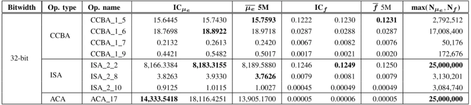
TABLE I
ESTIMATION RESULTS AND COMPARISON WITH EXHAUSTIVE CHARACTERIZATION FOR OPERATORS OF SMALL WORD-LENGTHS. Bitwidth Op. type Op. name ICµe µe ICf f max( Nµe, Nf)
8-bit ISA ISA 2 2 0.8633 0.9550 0.8750 0.1079 0.1194 0.1094 11,765 ISA 2 4 0.0416 0.1384 0.0938 0.0104 0.0346 0.0234 578 ACA ACA 6 1.6718 1.9856 1.7500 0.0151 0.0177 0.0156 35,873 16-bit CCBA CCBA 1 6 0.7299 0.8175 0.75 0.1825 0.2043 0.1875 5041 ISA ISA 2 4 1.9535 2.0568 1.9688 0.0305 0.0321 0.0308 178,930 ISA 2 6 0.1725 0.2688 0.2422 0.0054 0.0084 0.0076 11,602 ACA ACA 12 9.4957 9.9386 9.6875 0.0005 0.0005 0.0005 25,000,000 ACA 8 170.5876 172.4411 169.6680 0.0157 0.0158 0.0156 25,000,000 TABLE II
ESTIMATION RESULTS AND COMPARISON WITH5-MILLIONBALLSIMULATIONS FOR32-BIT OPERATORS.
Bitwidth Op. type Op. name ICµe µe5M ICf f 5M max( Nµe, Nf)
32-bit CCBA CCBA 1 5 15.6445 15.7430 15.7593 0.1222 0.1230 0.1231 2,792,512 CCBA 1 6 18.7698 18.8922 18.9718 0.0287 0.0288 0.0287 17,008,400 CCBA 1 7 0.2132 0.2613 0.2420 0.0067 0.0082 0.0076 50,176 CCBA 1 9 0.4421 0.5482 0.5017 0.0017 0.0021 0.0020 172,676 ISA ISA 2 2 8,166.3384 8,183.3155 8,189.5880 0.1246 0.1249 0.1250 25,000,000 ISA 2 8 3.8263 3.9330 3.7626 0.0079 0.0081 0.0079 3,130,201 ISA 2 10 0.9125 1.0115 1.0027 0.00045 0.00049 0.00049 3,084,740 ACA ACA 17 14,333.5418 18,116.4251 13,905.1700 0.00005 0.00006 0.00005 25,000,000
by the ACA and the ISA, depending of the number of cuts and cutting distance (main CCBA design parameters).
B. Results
The proposed experimental study aims at showing that 1) the CASSIS method correctly estimates error characteristics of circuits for various bitwidths, 2) this estimation keeps consistent for higher bitwidths where exhaustive simulation is not possible, and finally that 3) for the majority of inexact adders, CASSIS overcomes naive random BALL simulation. Two cases are shown: CASSIS requires less samples and thus converges faster towards an accurate error estimation, or CASSIS requires more samples than the traditional random BALL simulation which is, in this case, not accurate enough. Implementations of each above-mentioned adder architec-ture have been synthesized, varying their bitwidths, from 8 to 32 bits, as well as their main design parameters, in order to cover a large spectrum of error behaviors. CASSIS characterizations have been completed with h = 5 % and p = 95 % on an Intel Core i7-6700 processor.
1) Quality of the estimation for small word-lengths
To first check the quality of the CASSIS method, small word-length inexact adders have been characterized with CAS-SIS, as well as with an exhaustive characterization using BALL simulations to obtain their real error characteristics. Table I reports the obtained confidence intervals on µeand f , compared to their real values, and the numbers of samples N used by CASSIS. For both 8 and 16-bit adders, the CASSIS confidence intervals almost always contain the real values, demonstrating its accuracy. The ACA 8 is the only design
for which the CASSIS confidence intervals do not contain the real values (c.f. bold numbers), but the relative error between confidence interval bound and real value is extremely small.
For most operators, only a few tens of thousands of simu-lated samples were required to get precise error characteristics. For 16-bit ACA, the number of simulated samples has been saturated at 25 millions (c.f. bold sample number). Indeed, ACA adders have a large standard deviation in error values. Though, the CASSIS method outputs very accurate estimated values of f and µe. The largest relative error on the estimated values compared to the exhaustive characterization is on the estimation of f of the operator ACA 12, and is equal to 2.5%. 2) Consistency of the estimation for 32-bit operators
Table II reports the results for 32-bit inexact adder charac-terization. To check the consistency of the CASSIS method for this larger word-length, the CASSIS characterization has been compared to random BALL simulation with 5 million samples from [13], which is the typical inexact circuit characterization method.The chosen CCBA and ACA adders are Pareto-optimal designs for area/delay shown in the comparative study of [13]. Those adders are realistic designs to be implemented, and thus represent ideal subjects for CASSIS characterization.
In the case of 32-bit operators, it is to be noted that both characterizations (CASSIS and random BALL) are statistical estimates. In case the two methods do not converge towards the same estimation, bold numbers represent values obtained with higher amount of samples, assumed more accurate. For 2 out of 8 designs (CCBA 1 5 and ISA 2 8), the CASSIS confidence intervals obtained with less simulation samples
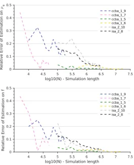
log10(N) - Simulation length 4 4.5 5 5.5 6 6.5 7 7.5 R elati ve Er ror of Esti mation on f 0 0.1 0.2 0.3 0.4 0.5 ccba_1_9 ccba_1_7 ccba_1_5 ccba_1_6 isa_2_10 isa_2_8
Fig. 1. Convergence of CASSIS estimation for µeand f with the number of
simulated samples N and with p = 95% and h = 0.5% for different 32-bit adders.
than the BALL method do not contain the error values from this latter. Nevertheless, the obtained estimated values of f and µe are very close from the random characterization. Inversely, for 3 of them (CCBA 1 6, ISA 2 2 and ACA 17), the CASSIS method has converged into different confidence intervals than the BALL simulation, as it has determined that more samples were required for safe estimation. This is coherent, as by user decision, the confidence interval has only 95 % chance to contain the real value. The most critical case concerns ACA 17. For this characterization, naive BALL simulation has dangerously underestimated µe compared to CASSIS. This is due to the very low error rate of the 32-bit ACA, for which 5 million samples is insufficient to make good statistics on errors.
3) Number of simulations required for accurate estimation Algorithm 1 implemented by CASSIS refines the estimation of µe and f given a refreshment period T . Fig. 1 illustrates the convergence of the estimation on µe and f . The different curves, corresponding to the different operators, have different starting points depending on the chosen T .
The final estimated values are all very accurate since the relative error of estimation is always lower than 0.1 %. Small bumps can be noted in the convergence of the estimated values due to the random sampling processed in each iteration of the algorithm. Besides, the speed of convergence strongly varies depending of the chosen operator. This is why an adaptive sample-size method like CASSIS better fits any operator rather than naive random BALL simulations.
IV. CONCLUSION
In this article, we proposed CASSIS, Characterization with Adaptive Sample-Size Inferential Statistics, a new method for the error characterization of inexact operators. From
user-defined confidence requirements, the CASSIS method auto-matically adjusts the number of simulations required by using statistical properties of the approximation error. This method is presented and demonstrated for the estimation of the error rate and mean error distance of various inexact adders. The CAS-SIS method has been applied to ACA, ISA and CCBA circuits, three major types of inexact adders. Validated by its accurate estimation of error characteristics on 8 to 16-bit circuits, CASSIS has been proven coherence and consistency on larger word-lengths, with 32-bit circuits, where exhaustive simulation is not feasible. This experimental study has demonstrated that CASSIS overcomes naive random BALL simulations with a fixed number of samples, either by converging towards a more accurate characterization, or by drastically reducing the amount of samples required for an accurate estimation, saving time and resources. As a future work, the proposed method will be validated on various approximate computing techniques.
This project has received funding from the French Agence Nationale de la Recherche under grant ANR-15-CE25-0015 (ARTEFaCT project).
REFERENCES
[1] K. Shi, D. Boland, and G. A. Constantinides, “Accuracy-performance tradeoffs on an FPGA through overclocking,” in IEEE FCCM, 21st Annual International Symposium on, 2013, pp. 29–36.
[2] A. Mercat, J. Bonnot, M. Pelcat, K. Desnos, W. Hamidouche, and D. Menard, “Smart search space reduction for approximate computing: A low energy hevc encoder case study,” JSA, vol. 80, pp. 56–67, 2017. [3] T. Liu and S.-L. Lu, “Performance improvement with circuit-level
speculation,” in IEEE/ACM MICRO 2000, 2000, pp. 348–355. [4] A. K. Verma, P. Brisk, and P. Ienne, “Variable latency speculative
addition: A new paradigm for arithmetic circuit design,” in Design, Automation and Test in Europe (DATE). IEEE, 2008, pp. 1250–1255. [5] V. Camus, J. Schlachter, and C. Enz, “Energy-efficient inexact specula-tive adder with high performance and accuracy control,” in Circuits and Systems (ISCAS), IEEE International Symposium, 2015.
[6] N. Zhu, W.-L. Goh, and K.-S. Yeo, “An enhanced low-power high-speed adder for error-tolerant application,” in Integrated Circuits (ISIC), 12th IEEE International Symposium on, Dec. 2009, pp. 69–72.
[7] V. Camus, J. Schlachter, and C. Enz, “A low-power carry cut-back approximate adder with fixed-point implementation and floating-point precision,” in Design Automation Conference (DAC), 2016.
[8] C. Liu, J. Han, and F. Lombardi, “An analytical framework for evaluating the error characteristics of approximate adders,” IEEE Transactions on Computers (TC), vol. 64, no. 5, May 2015.
[9] Y. Wu, Y. Li, X. Ge, and W. Qian, “An accurate and efficient method to calculate the error statistics of block-based approximate adders,” arXiv preprint arXiv:1703.03522, 2017.
[10] S. Mazahir, O. Hasan, R. Hafiz, M. Shafique, and J. Henkel, “Proba-bilistic error modeling for approximate adders,” IEEE Transactions on Computers (TC), vol. 66, no. 3, pp. 515–530, 2017.
[11] K. Du, P. n, and K. Mohanram, “High performance reliable variable latency carry select addition,” in IEEE DATE, 2012, pp. 1257–1262. [12] H. Jiang, C. Liu, L. Liu, F. Lombardi, and J. Han, “A review,
classifica-tion and comparative evaluaclassifica-tion of approximate arithmetic circuits,” in ACM Journal on Emerging Technologies in Computing Systems (JETC), 2017.
[13] V. Camus, M. Cacciotti, J. Schlachter, and C. Enz, “Design of approx-imate circuits by fabrication of false timing paths: The carry cut-back adder,” in IEEE Journal on Emerging and Selected Topics in Circuits and Systems (JETCAS), 2018.
[14] G. Demengel, P. B´enichou, and N. Boy, Probabilit´es, statistique inf´erentielle, fiabilit´e : outils pour l’ing´enieur., ser. Math´ematiques appliqu´ees. Paris : Ellipses. impr. 1997, cop. 1997., 1997.