A Geometry Driven Reconstruction Algorithm for the Mojette Transform

(1)

HAL Id: hal-00267628

https://hal.archives-ouvertes.fr/hal-00267628

Submitted on 27 Mar 2008

HAL is a multi-disciplinary open access

archive for the deposit and dissemination of

sci-entific research documents, whether they are

pub-lished or not. The documents may come from

teaching and research institutions in France or

abroad, or from public or private research centers.

L’archive ouverte pluridisciplinaire HAL, est

destinée au dépôt et à la diffusion de documents

scientifiques de niveau recherche, publiés ou non,

émanant des établissements d’enseignement et de

recherche français ou étrangers, des laboratoires

publics ou privés.

A Geometry Driven Reconstruction Algorithm for the

Mojette Transform

Nicolas Normand, Andrew Kingston, Pierre Évenou

To cite this version:

Nicolas Normand, Andrew Kingston, Pierre Évenou. A Geometry Driven Reconstruction Algorithm

for the Mojette Transform. Discrete Geometry for Computer Imagery, Oct 2006, Szeged, Hungary.

pp.122-133, �10.1007/11907350_11�. �hal-00267628�

(2)

A geometry driven reconstruction algorithm for the Mojette transform

Nicolas Normand, Andrew Kingston, Pierre ´Evenou IRCCyN/IVC UMR CNRS 6597

Abstract. The Mojette transform is an entirely discrete form of the Radon transform developed in 1995. It is exactly invertible with both the forward and inverse transforms requiring only the addition opera-tion. Over the last 10 years it has found many applications including image watermarking and encryp-tion, tomographic reconstrucencryp-tion, robust data transmission and distributed data storage. This paper presents an elegant and efficient algorithm to directly apply the inverse Mojette transform. The method is derived from the inter-dependance of the “rational” projection vectors (pi, qi) which define the direc-tion of projecdirec-tion over the parallel set of lines b = pil− qik. Projection values are acquired by summing the value of image pixels, f(k, l), centered on these lines. The new inversion is up to 5 times faster than previously proposed methods and solves the redundancy issues of these methods.

@inproceedings{normand2006dgci,

Author = {Normand, Nicolas and Kingston, Andrew and {\’E}venou, Pierre}, Booktitle = {Discrete Geometry for Computer Imagery},

Date = {2006-10},

Doi = {10.1007/11907350_11},

Editor = {Kuba, Attila and Ny{\’u}l, L{\’a}szl{\’o} G. and Pal{\’a}gyi, K{\’a}lm{\’a}n}, Month = oct,

Pages = {122-133},

Publisher = {Springer Berlin / Heidelberg}, Series = {Lecture Notes in Computer Science},

Title = {A Geometry Driven Reconstruction Algorithm for the {M}ojette Transform}, Volume = {4245},

Year = {2006}}

(3)

A geometry driven reconstruction algorithm for

the Mojette transform

Nicolas Normand, Andrew Kingston and Pierre ´Evenou

IRCCyN-IVC, ´Ecole polytechnique de l’Universit´e de Nantes,

Rue Christian Pauc, La Chantrerie, 44306 Nantes Cedex 3, FRANCE.

{nicolas.normand,andrew.kingston,pierre.evenou}@univ-nantes.fr

Abstract. The Mojette transform is an entirely discrete form of the Radon transform developed in 1995. It is exactly invertible with both the forward and inverse transforms requiring only the addition operation. Over the last 10 years it has found many applications including image watermarking and encryption, tomographic reconstruction, robust data transmission and distributed data storage. This paper presents an elegant and efficient algorithm to directly apply the inverse Mojette transform. The method is derived from the inter-dependance of the “rational” pro-jection vectors (pi, qi) which define the direction of projection (by sum-ming the value of image pixels, f (k, l), centered) on the parallel set of lines b = pil− qik. It is up to 5 times faster than previously proposed methods and solves the redundancy issues of these methods.

1 Introduction

The Mojette transform is a form of Radon transform. It is an entirely discrete mapping which requires only the addition operation and is exactly invertible. It was first proposed by Gu´edon, Barba and Burger in 1995 [1] in the context of psychovisual image coding. It has since been applied in many aspects of image processing such as image analysis [2], image watermarking [3], image encrytion [4], image compression [5] and tomographic image reconstruction from projec-tions [6, 7]. The unique properties of the transform have also made it a useful multiple description tool with applications in robust data transmission [8] and distributed data storage [9]. A summary of the evolution and applications of the mojette transform entitled “The Mojette Transform: the Fist Ten Years” [10] was presented at the last DGCI conference.

Since the Mojette transform is pre-dominantly used as a tool, (e.g., for image analysis, to apply a watermark, for channel coding), the transform and inversion procedure should be as efficient as possible especially for real-time applications. This paper presents a inversion algorithm which uses a geometrical approach to streamline the reconstruction process.

Section 2 recalls the definition and some important properties of the Mojette transform as well as the methods for exact inverse utilised to date. Section 3

(4)

outlines the proposed geometry driven inversion method initially for simple cases where qi or pi is constant for all I projections and then generalises the results

to an arbitrary set of (pi, qi). A comparison between this method and previously

proposed reconstructions is presented in Section 4 followed by a conclusion in Section 5.

2 The Mojette Transform

2.1 The forward transform (Projection)

The linear integration of the discrete 2D function f(k, l) is obtained via the Mojette transform over a set of I pre-defined rational angles, θi= tan−1(qi/pi).

The pairs of integers defining the angles, (pi, qi) must be relatively prime, i.e.,

gcd(pi, qi) = 1, and since linear integration is directionally independant, qi is

restricted to Z+ _{(except for the case p}

i = 1, qi = 0) to ensure θi ∈ [0, π[.

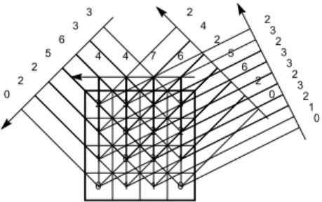
Assuming a Dirac pixel model the linear integrations become sums over the pixels centred on the lines b = qik− pil. The Mojette projection operator is

defined as M{f(k, l)} = Proj(pi, qi, b) = P_!−1 k=0 Q−1_! l=0 f (k, l)δ(b + pil− qik), (1)

where δ(η) is the Kronecker function, i.e., δ(η) = 1 if η = 0, otherwise δ(η) = 0. An example of these projections is given in Fig. 1. The number of linesums called “bins” per projection, B, for a P × Q image is found as

Bi(P, Q, pi, qi) = (Q − 1)|p| + (P − 1)q + 1, (2)

with b ∈ [0, Bi− 1] for pi ≤ 0 and b ∈ [−(Q − 1)pi, (P − 1)qi] otherwise. For

a transform with I projections, unique inversion is possible provided the Katz criterion [11] is satisfied, i.e.,

P _≤ I−1 ! i=0 |pi| or Q ≤ I−1 ! i=0 qi. (3)

This criterion was generalised by Normand, Gu´edon, Phillip´e and Barba [12] for images of arbitrary shape. Their scheme generates the minimum sized ghost functions ,(i.e., functions that exist in the image but disappear in the projections, refer to [11] for more detail) as a sequence of 2D convolutions with all two pixel structuring elements formed from the set of projection slopes qi/piby 1 at (0, 0)

and -1 at (pi, qi). Any array which cannot contain the minimum ghost generated

by the projection set therefore has an empty null-space and must have a unique inverse.

(5)

T2/8 1. Fig 1 - Forward projection

T3/8 2. Fig 2 - Reconstruction Step

Fig. 1. Four projections of a 4×4 image f(k, l), Proj(−1, 1, b), Proj(0, 1, b), Proj(1, 1, b) and Proj(2, 1, b).

2.2 The inverse transform (Reconstruction)

When the Mojette transform was first proposed a recursive algebraic method was used for reconstruction. The following year a fast and more direct technique, requiring addition operations only was proposed by Normand, Gu´edon, Philipp´e and Barba [12]. It solves for one pixel at a time and subtracts this value from the bins that include this pixel in each of the I projections [12]. The reconstruction propagates from the image corners (where there is only one pixel value in the bins) to the centre. The first step of the inversion for f(k, l), as given in Fig. 1, is shown in Fig. 2a. For each of the P Q pixels there are O(I) operations, so the complexity of this technique is O(IP Q). If the number of projections, I, is chosen to be log(P Q), the Mojette transform has similar complexity to that of the fast Fourier transform [12].

There are two minor problems with this method. First, locating the bins in a projection which can be back projected (i.e., those bins for which only one pixel value remains unknown its corresponding line of projection). Second, determining which one of the pixels, (k, l), in the line of projection, b = qik−pil,

is yet to be reconstructed.

A simple method is utilised to overcome these problems. Two “comptabilit´e” (or accounting) images are projected with the same projection sets and recon-structed simultaneously with the unknown image. The first of these is a unitary

image, i.e., an image where f(k, l) = 1 for all pixels. The second is an index image which labels the pixels according to a raster scan, i.e., f(k, l) = k + lP .

The projections of these images assist with the respective problems above. This inversion technique will be referred to as the Comptabilit´e Mojette Inversion (CMI) method.

In recent years, two back-projection reconstruction methods have been pro-posed in the context of applying the Mojette transform to reconstruct medical images from continuous projections. The first of these is an exact method which was discovered by Servi`eres, Normand, Gu´edon and Bizais [7]. Given all I pos-sible projections in the P × Q array, back-projection (M∗_{) yields I − 1 times}

(6)

(a)

(b)

(c)

Fig. 2. Reconstructon via the CMI method. (a) A candidate bin is selected in the projections of the unitary image. (b) The value in the corresponding projection bin of the index image gives the pixel to be reconstructed. (c) The value in the corresponding projection bin of the image gives the pixel value. The projections of all 3 images are then updated simultaneously.

"

bProj(pi, qi, b) for any projection), i.e.,

M∗_{Proj(p i, qi, b)} = ˜f (k#, l#) = I−1_" i=0 Proj(pi, qi, qik− pil) =I"−1 i=0 f (k, l)δ(qi(k − k#) − pi(l − l#)) = (I − 1)f(k#_{, l}#_{) + f} sum. (4)

The set of projections can be found from (pi, qi) being all the points visible from

the origin, i.e., Farey points, of the P × Q array and all symmetries, (−pi, qi).

Assuming a uniform density of Farey points in the plane, approximately I = 12P Q/π2 _{projections are required.}

The second back-projection technique uses the conjugate gradient method [13] to minimise ||M∗_b_{− M}∗_{M ˜}_f_||2 _{where ˜}_{f is the reconstructed image. Both}

of these inversions are relatively stable in the presence of noise and therefore ideal in this context. The exact back-projection however requires a very large number of projections and the conjugate gradient method, while it does give the inverse, is unnecessary in the case of reconstruction from uncorrupted discrete projections.

Since the Mojette transform is often used as a CoDec in data transmission, the most efficient inversion possible is required for real time applications. The following section outlines a very efficient inversion method which is similar to the CMI method but determines the inter-dependance of projections using graph theory to remove the accounting problems.

3 A Geometry Driven Reconstruction

For this method of reconstruction, it is assumed that "I−1

i=0 qi= Q. Any

redun-dant projections are ignored. The reconstruction is performed from left to right, (reconstruction from right to left, top to bottom and bottom to top are symme-tries of this method). These two properties imply this algorithm can reconstruct

(7)

images of infinite size, “on the fly”, only the image height Q must be finite, P is not restricted.

When reconstructing an image (according to the above criteria) using the CMI method, the reconstruction can be seen to originate in the image corners retaining a convex region of unknown pixel values and then propagates towards the right. Once the initial trivial section in the corners is completed, it can be noticed that the projections and image rows are linked in that the same projection is utilised to reconstruct the next pixel in the same row. The algorithm proposed here takes advantage of this. To describe how, it is preferable to begin with a simplified case where all projections have a common value for qi of 1.

3.1 The case where qi = 1 for i ∈ ZQ

This case commonly arises when the Mojette transform is utilised for multiple description coding in packet data transmission [8]. If the set of projections are sorted by pi, (i.e., p0 < p1 < . . .), and reconstruction is performed from left

to right, then row r of the image, f(k, r) for k ∈ ZP, is reconstructed by the

Mojette projection, Proj(pr, 1, b).

Proof. Assume on the contrary that projection, Proj(pQ−1, 1, b), is used to

re-construct the pixel value f(k, l) on a row other than Q − 1, i.e., 0 ≤ l < Q − 1. This implies that the pixel value f(k+pQ−1, l+1) has already been reconstructed

by some projection other than Proj(pQ−1, 1, b), say Proj(pr, 1, b). Thus the pixel

value f(k + pQ−1− pr, l) must have been reconstructed and since pQ−1 is the

largest in the set of pi, then k + pQ−1− pr > k and this pixel is further right

than f(k, l). However, it can not be known if reconstructing from left to right; A contradiction.

Therefore, only row Q − 1 can be reconstructed by Proj(pQ−1, 1, b). Since

reconstruction requires that only one pixel remains unknown in the line of pro-jection, Proj(pQ−1, 1, b) can not be used to reconstruct any other row. Therefore,

this proof can be repeated to show Proj(pQ−2, 1, b) must reconstruct row Q− 2

and so on, down to Proj(p0, 1, b).

Intuitively this can be seen as ordering the projections by the slope (or an-gle) of their corresponding line of projection. This gives a convex hull to the reconstruction region that ensures the lines of back-projection can cut the hull such that only one pixel on the line lies within the hull; The condition necessary for reconstruction.

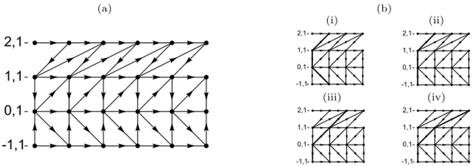
Since each projection corresponds to a one row of the image, a dependancy graph can be constructed to show the relationship between the projections in reconstruction. The dependancy graph for the example image of Fig. 1 is given in Fig. 3a. Here vertices correspond to pixels and directed edges represent the dependancies of each pixel on other pixels being reconstructed in the inversion process.

Two simple paths can be found to traverse the graph (as shown in Fig. 3b-i and b-3b-iv for the example). The reconstruct3b-ion process 3b-involves beg3b-inn3b-ing to

(8)

(a)

T1/6

(b) (i) T4/6 3. Fig 4 - DependancyGraph_p3_q3 T5/6 4. Fig 3 - DependancyGraphRDV (ii) T4/6 3. Fig 4 - DependancyGraph_p3_q3 T5/6 4. Fig 3 - DependancyGraphRDV (iii) T4/6 3. Fig 4 - DependancyGraph_p3_q3 T5/6 4. Fig 3 - DependancyGraphRDV (iv) T4/6 3. Fig 4 - DependancyGraph_p3_q3 T5/6 4. Fig 3 - DependancyGraphRDV

Fig. 3. (a) The dependancy graph for the example image. (b) The 4 possible recon-struction paths

the left of the image, so that only the rightmost of the vertices in the path intersect image pixels in column zero, and reconstructing pixel values according to the path. The distance the path is initially shifted is referred to as the offset. The path is then shifted right 1 pixel and the entire process repeated until the last pixel value in column P − 1 of image is reconstructed. This process will be referred to as the Balayage (or sweeping) Mojette Inversion (BMI) method.

The path through the graph termed a reconstruction path does not necessarily have to traverse from one side to the other. Two seperate paths originating from opposite sides of the graph can terminate at a common vertex in the graph (some examples are shown in Fig. 3b-ii and b-iii). To optimise the reconstruction algorithm, it is desired to find the most compact path possible.

The offset for two paths in the graph terminating on row r due to all projec-tion vectors with negative gradient is found as

Offset−_{(r) =} "r i=1max(0, −p i) + Q_"−2 i=rmax(0, −p i) = max(0, −pr) + Q_"−2

i=1 max(0, −pi) = max(0, −pr

) + S−_,

(5)

where S−_{= "}Q−2

i=1 max(0, −pi). Similarly the offset due to all projection vectors

with positive gradient is found as: Offset+_{(r) =}"r i=1 max(0, pi) + Q_"−2 i=r max(0, pi) = max(0, pr) + Q_"−2 i=1 max(0, pi) = max(0, pr) + S+, (6) where S+ _{= "}Q−2

i=1 max(0, pi). The width of the reconstructed path is

deter-mined by the maximum of these two offsets. The objective is therefore to find an r which minimises

(9)

Let S = S−_−S+_{= "}Q−2

i=1 −pi. Note that if S− > S+then any pr∈ [0, S] has

no effect on Offsettotal. Similarly, if S−< S+ then any pr ∈ [S, 0] has no effect

on Offsettotal. Therefore the optimal pr lies in the range [min(0, S), max(0, S)].

If there is no pr within this range then that which is minimises the following

should be selected; # pr− min(0, S) + max(0, S) 2 $2 = (pr− 0.5S)2. (8)

Balayage Inversion Algorithm(for qi= 1 for i ∈ ZI)

! Input: Set of projections, Proj(pi, 1, b), ordered with increasing pi

! Output: Reconstructed image, f(k,l).

Begin

2 % Compute S−_{, S}+ _{and S}

2 S minus ← S plus ← 0

3 for i ← 1 to Q − 2 do

4 S minus_{← S minus + max(0, −p}i)

5 S plus_{← S plus + max(0, p}i)

6 S¯_{← S minus − S plus}

% Determine the rendezvous row r

7 temp ← (p0− 0.5S)2 8 r_{← 0} 9 for i ← 1 to Q − 1 do 10 if (pi− 0.5S)2< temp then 11 temp ← (pi− 0.5S)2 12 r← i ¯ ¯

% Determine the initial image column offset for each projection

13 offset(r) ← max(max(0, −pr) + S minus, max(0, pr) + S plus)

14 for i ← r + 1 to Q − 1 do 15 offset(i) ← offset(i − 1) + pi−1

16 for i ← r − 1 downto 0 do¯ 17 offset(i) ← offset(i + 1) + pi+1

¯

% Begin reconstructing image, f (k, l), at column k =_−offset(r)

18 for k ← −offset(r) to P − 1 do 19 for l ← 0 to r − 1 do 20 f (k, l)_{← Proj}l(k − pkl) 21 for i ← 0 to Q − 1 do 22 Proj_i(k − pil)← Proji(k − pil)− f(k, l) 23 for l ← Q − 1 downto r do¯ ¯ 24 k#← k + offset(r) − offset(l) 25 f (k#, l)← Projl(k#− pkl) 26 for i ← 0 to Q − 1 do 27 Proj_i(k#_{− p}il)← Proji(k#− pil)− f(k#, l) 28 End¯ ¯ ¯

This reconstruction procedure can be trivially generalised to the case where all qi= m for m ∈ Z+. In this instance each projection Proj(pi, m, b) reconstructs

(10)

m consecutive rows of the image. The reconstruction paths are simlar to that

for the above case with qi= 1 but with m passes shifted down a row each time.

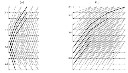
An example directed graph and reconstruction path for m = 3 is presented in Fig. 4a. Another simple case for the reconstruction occurs when pi is constant

for all projections as is discussed in the next section. 3.2 The case where pi = m for i ∈ ZI

This case where m = 1 is the most common type of angle set used for transform-ing images with minimal redundancy as described in [12]. Since pi is constant,

for a proof similar to that given in section 3.1 to apply, the projections must be sorted in order of decreasing qi, (i.e., q0> q1> . . .), then the rth set of qi rows

of the image, i.e., from row R + 1 up to row R + qr where R = "r−1i=0qi, are

reconstructed by projection Proj(m, qr, b).

Since all qi> 0 the set of reconstruction paths all have the same total offset

of (I − 1)m as shown for the example in Fig. 4b. The reconstruction is similar to that for constant qi, in that it requires multiple passes (qmax in this case),

however the number of vertices included in each subsequent pass decreases as shown for the example.

(a) Fig 4a Fig 4b T6/8 5. Fig 4 - DependancyGraph_p3_q3 T7/8 6. Fig 5 - DependancyGraph_varying_pq (b) Fig 4a Fig 4b T6/8 5. Fig 4 - DependancyGraph_p3_q3 T7/8 6. Fig 5 - DependancyGraph_varying_pq

Fig. 4. The dependancy graphs (grey) and simplest reconstruction paths (black) for the set of projections (a) Proj(Proj(_{−2, 3, b), Proj(−1, 3, b), Proj(1, 3, b) and Proj(2, 3, b)} which requires 3 passes and (b) Proj(3, 1, b), Proj(3, 2, b), Proj(3, 4, b) and Proj(3, 5, b)

which requires qmax= 5 passes.

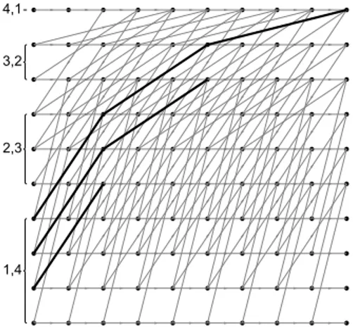
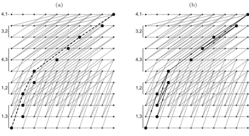
3.3 The case where pi ≥ pi−1 and qi≤ qi−1

The constant qi and constant pi cases from Sections 3 and 3.2 can be

(11)

increasing and qi is decreasing, i.e., pi≥ pi−1 and qi ≤ qi−1 for (0 < i < I). For

this case the reconstruction path is straightforward, similar to that for constant

pi path with qmax passes. The paths through the region with pi ≥ 0 can be

constructed independantly to those in the region with pi≤ 0 similar to the case

with constant qi. An example has been presented in Fig. 5.

Fig 4a

Fig 4b

T6/8

5. Fig 4 - DependancyGraph_p3_q3

T7/8 6. Fig 5 - DependancyGraph_varying_pq

Fig. 5. The dependancy graph for the set of projections Proj(4, 1, b), Proj(3, 2, b), Proj(3, 2, b) and Proj(4, 1, b) with the simplest reconstruction path shown in black

which requires qmax= 4 passes.

3.4 The general case

The above reconstruction techniques can be generalised to any set of I projec-tions such that "I−1

i=0 qi= Q for qi∈ Z+. As for the previous cases with varying

qi, if the set of projections are sorted by slope pi/qi, (i.e., p0/q0< p1/q0< . . .),

then the rth _{set of q}

i rows of the image are reconstructed by the Mojette

pro-jection, Proj(pr, qr, b). The proof is again similar to that given in section 3.1.

Since each projection corresponds to qi rows of the image, once again a

dependancy graph can be constructed to show the relationship between the projections in reconstruction. However, each vertex of the graph is no longer assured of 2 originating and 2 terminating directed edges. There may only be a single terminating edge and there may be zero or many originating edges depending on the set of (pi, qi) used to define the projections.

To ensure a reconstruction path in this instance, only the pixels located immediately inside the edge of the convex hull created by the lines of projection ordered by slope are considered. As for the constant qi case, the paths that

terminate at the rows with minimum slope are used to generate the most compact convex hull. An example of the selection process is given in Fig. 6a with the

(12)

dashed line giving the complex hull. The directed graph is then used to determine the reconstruction paths required for these selected vertices as shown in Fig 6b for the example.

(a)

Fig 6a

Fig 6b

T8/8 7. Fig 6 - DependancyGraph_any_pq (b)

Fig 6a

Fig 6b

T8/8 7. Fig 6 - DependancyGraph_any_pq

Fig. 6. Determining the vertices of the dependancy graph to be considered for the set of projections (a) Proj(Proj(4, 1, b), Proj(3, 2, b), Proj(4, 3, b),Proj(1, 2, b) and Proj(1, 3, b) (b) A reconstruction path from the directed graph to reconstruct these vertices.

4 Discussion

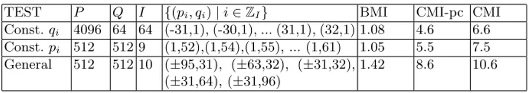
Although very similar in nature, the balayage inversion algorithm can be shown to be up to 5 times faster than the comptabilit´e inversion algorithm. Assuming the pixel count and pixel label projections have not been pre-computed (which is possible in the case of image transmission where the incoming array size is known), these must both be determined in 2×O(P QI) operations and during the inversion process, I projection value bins, pixel count bins and pixel label bins must be updated for each of the P × Q pixels (3 × O(P QI) operations), giving a total of approximately 5×O(P QI) operations. In contrast the balayage algorithm requires updating I projection bins for each image pixel once in a single pass across the image in O((P + Offset)QI) operations. This has been demonstrated for three types of angle sets in Table 1 comparing the computation times for the BMI, the CMI with pre-computed unitary and index image projections (CMI-pc) and the complete CMI. In implementation the actual gain in efficiency can be up to an order of magnitude since there is a periodic pattern to the BMI process that can be exploited while this is not the case for the CMI method where the position of the next pixel to be reconstructed is not predetermined at all.

(13)

TEST P Q I {(pi, qi)| i ∈ ZI} BMI CMI-pc CMI Const. qi 4096 64 64 (-31,1), (-30,1), ... (31,1), (32,1) 1.08 4.6 6.6 Const. pi 512 512 9 (1,52),(1,54),(1,55), ... (1,61) 1.05 5.5 7.5 General 512 512 10 (_{±95,31), (±63,32), (±31,32),} (_{±31,64), (±31,96)} 1.42 8.6 10.6

Table 1. Reconstruction times comparing the BMI with CMI-pc (pre-computed uni-tary and index image projections) and CMI methods. Times are given as a ratio with respect to the time to perform the forward Mojette transform.

Since the proposed method is based on the inter-dependancy of each projec-tion, the algorithm removes the need to search through the projections to find the next candidate bin that can be back-projected. As a pixel is reconstructed the predetermined dependancy graph indicates the pixel that can be reconstructed next and by what projection. This is highlighted by the relative performance of the CMI method for the General case of Table 1 where the projections have a large number of possible reconstruction bins to manage. The CMI algorithm is more robust however, it is more adaptable to any set of projections such as redundant sets where "I−1

i=0 qi> Q and sets of partial projection data.

The knowledge of which projections are used to reconstruct which rows of the image can be also used to ignore/discard projection bins that are not required for the inversion. This removes unwanted redundancy to optimise Mojette encoding as was investigated by Verbert, Ricordel and Gu´edon in [14].

5 Conclusion and Future Work

A new inversion algorithm for the Mojette transform has been presented which takes advantage of the knowledge of the interdependancy of projections in recon-struction. The method is more direct and more efficient than previous methods however is less robust in terms of adaptability to any set of projections. This method of reconstruction also automatically enables optimal encoding by the Mojette transform by identifying which projection bins are required for inver-sion. Developing a BMI method that can be applied to reconstruct a redundant set of projections and can adapt to sets of partial projections as well as deter-mining optimal coding incorporating redundancy are topics of future research.

Acknowledgements

AK holds a postdoctoral position at l’Universit´e de Nantes supported by a grant from the R´egion Pays de la Loire, France.

(14)

References

1. Gu´edon, J., Barba, D., Burger, N.: Psychovisual image coding via an exact dis-crete Radon transform. In Wu, L., ed.: Proc. Visual Communications and Image Processing 1995 (VCIP95), Taipei, Taiwan, CORESA (1995) 562–572

2. Gu´edon, J., Normand, N.: The Mojette transform: applications in image analysis and coding. The International Society for Optical Engineering 3024(2) (1997) 873–884

3. Autrusseau, F., Gu´edon, J.: Image watermarking for copyright protection and data hiding via the Mojette transform. In Sonka, M., Fitzpatrick, J., eds.: Proc. SPIE; Security and Watermarking of Multimedia Contents IV. Volume 4675., San Jose, CA (2002) 378–386

4. Autrusseau, F., Gu´edon, J., Bizais, Y.: Mojette cryptomarking scheme for medical images. In Sonka, M., Fitzpatrick, J., eds.: Proc. SPIE; Medical Imaging 2003: Image Processing. Volume 5032. (2003) 958–965

5. Autrusseau, F., Parrein, B., Servi`eres, M.: Lossless compression based on a discrete and exact Radon transform: A preliminary study. In: Proc. IEEE International Conference on Acoustics, Speech and Signal Processing 2006 (ICASSP), Toulouse, France (2006)

6. Servi`eres, M., Gu´edon, J., Normand, N.: A discrete tomography approach to PET reconstruction. In: Proc. 7th International Conference on Fully 3D Reconstruction in Radiology and Nuclear Medicine, Saint-Malo, France (2003)

7. Servi`eres, M., Normand, N., Gu´edon, J., Bizais, Y.: The Mojette transform: Dis-crete angles for tomography. In Herman, G., Kuba, A., eds.: Proc. of Workshop on Discrete Tomography and its Applications, New York City, Elsevier Science Publishers (2005)

8. Parrein, B., Gu´edon, J., Normand, N.: Multimedia forward error correcting codes for wireless LAN. Annals of Telecommunications 3(4) (2003) 448–463

9. Gu´edon, J., Parrein, B., Normand, N.: Internet distributed image information system. Integrated Computer-Aided Engineering 8 (2001) 205–214

10. Gu´edon, J., Normand, N.: The Mojette transform: the first ten years. In Andres, E., Damiand, G., Lienhardt, P., eds.: Proc. 12th International Conference on Discrete Geometry for Computer Imagery. Volume LNCS3429., Poitiers, France, Springer-Verlag (2005) 79–91

11. Katz, M.: Questions of uniqueness and resolution in reconstruction from projec-tions. Springer Verlag (1977)

12. Normand, N., Gu´edon, J., Philipp´e, O., Barba, D.: Controlled redundancy for image coding and high-speed transmission. In Ansari, R., Smith, M., eds.: Proc. SPIE Visual Communications and Image Processing 1996. Volume 2727., SPIE (1996) 1070–81

13. Servi`eres, M., Idier, J., Normand, N., Gu´edon, J.: Conjugate gradient Mojette reconstruction. In Fitzpatrick, J., Reinhardt, J., eds.: Proc. SPIE Medical Imaging 2005: Image Processing. Volume 5747. (2005) 2067–74

14. Verbert, P., Ricordel, V., Gu´edon, J.: Analysis of the Mojette transform projections for an efficient coding. In: Proc. International Workshop on Image Analysis for Multimedia Interactive Services (WIAMIS), Barcelona, Spain (2004)