Regional analysis and modelling of water temperature metrics for Atlantic Salmon (Salmo salar) in Eastern Canada. Final report.

REGIONAL ANALYSIS AND MODELLING OF WATER TEMPERATURE

METRICS FOR ATLANTIC SALMON (SALMO SALAR) IN EASTERN

CANADA: FINAL REPORT

C. Charron

_{, A. St-Hilaire}

_{, C. Boyer}

_{, A. Daigle}

_,

T. B.M.J. Ouarda

_{, N.E. Bergeron}

_,

1.

INRS-ETE, Québec City, 490 de la Couronne, Québec City, Qc, G1K 9A9

Centre Interuniversitaire de recherche sur le saumon Atlantique

April 2020

© INRS, Centre - Eau Terre Environnement, 2021

Tous droits réservés

ISBN : 978-2-89146-947-0 (version électronique)

Dépôt légal - Bibliothèque et Archives nationales du Québec, 2021

Dépôt légal - Bibliothèque et Archives Canada, 2021

Table of Content

Part A: Project Information ... 4

PART B: Project Objectives and Results ... 4

1. Project Objectives ... 4 2. Expected Results ... 4 PART C: Reporting ... 4 3. Results Achieved ... 4 4. Anticipated Risks ...18 5. Data Dissemination ...19 6. Publications ...19 7. Statement of Accounts ...19

List of figures

Figure 1. Gaussian functions fitted to daily interannual mean water temperatures to

estimate the uncertainty of parameters a, b and c (from Daigle, Boyer, and St-Hilaire

(2019)). ... 7

Figure 2. Dendrograms with cut-off thresholds for a) MeanWaterTmax; b)

Max_Num_Day; c) Gaussian_a; d) Gaussian_b; c) Gaussian_c. Note that not all station

numbers are shown on the x-axis. ... 11

Figure 3. Maps of stations grouped using HCA-GAM for a) MeanWaterTmax; b)

Max_Num_Day; c) Gaussian_a; d) Gaussian_b; c) Gaussian_c. ... 13

Figure 4. Scatter plots of observed vs. simulated values of temperature metrics for MLR.

... 15

Figure 5. Scatter plots of observed vs. simulated values of temperature metrics for

GAM. ... 16

Figure 6. Splines for the predictors used in the GAM-ALL model. ... 17

List of Tables

Table 1. Selected predictors when all stations were grouped together. ... 8 Table 2. Performance metrics for different Regional Thermal Analysis methods in Atlantic salmon rivers ... 14

Part A: Project Information

Project Title:

Predicting hydro-thermal conditions in Atlantic salmon rivers using regional analysis in a

changing climate.

Project Lead:

André St-Hilaire

Collaborators: Christian Charron, Claudine Boyer, Anik Daigle, Taha B.M.J. Ouarda and

Normand E. Bergeron.

Name of Organization:

Institut National de la Recherche Scientifique, Centre Eau Terre Environnement

(INRS-ETE)

Term of the Agreement

From [04/2018] – to [03/2020]

Contribution Period (Final)

From [04/2019] – to [03/2020]

PART B: Project Objectives and Results

 To define homogenous hydro-thermal regions in Eastern Canadian salmon rivers.

 To provide scenarios of expected changes in Atlantic salmon freshwater habitat in Eastern

Canada.

2. Expected Results



A first complete methodology for the delineation of hydro-thermal regions for Atlantic

salmon rivers.



The inclusion of groundwater as a key variable in the definition of hydro-thermal regions

and for the consideration of climate change impacts.



Thermal and hydrological models that are calibrated and optimized for each region.



Scenarios of future Atlantic salmon habitat conditions in Eastern Canadian rivers and how

they may affect salmon production.

PART C: Reporting

Given that the funding received did not allow for the implementation of the full proposal, the work focused on the first objective stated in Part B, Section 1 and the first expected result of Section 2. The following sub-sections provide a summary of the methodology and final results.

3.1 Methods

The details of the methods used in the study were presented in Charron et al. (2019). In order to facilitate reading and interpreting the results presented herein, a summary of the methods is repeated in the following paragraphs.

The main methodological difference between the present study and that of Charron et al. (2019) is the water temperature database. In the 2019 study, the main criterion for selecting water temperature stations for the regional analysis was that the length of the time series was five years or more. In the present report, this criterion was relaxed to four summers (30 June-1 Sept as a minimum duration). The second criterion that was applied in this new study was to eliminate redundant stations. As shown in Figure 1 of Charron et al. (2019), some rivers included in the study are monitored using a network of stations with a finer spatial resolution than others (e.g. Ouelle, Restigouche and Ste-Marguerite rivers), resulting in over twenty stations on some rivers, with highly redundant information for regional analysis. In order to alleviate this problem, only one station was retained on most rivers. However, in order to lengthen the time series used in the study, where possible, daily water temperature series at the site selected for the study were extended using linear regression with neighbouring water temperature stations. The criteria used to decide if this data transfer was to be performed were:

 The concomitant period between the two stations was > 300 days OR the concomitant period was > 100 days AND the distance between the two stations was < 5 km.

 The Root Mean Square Error (RMSE) of the regression was < 0.5°C.  The 95th _{percentile of the absolute regression error was < 1°C.}

For 11 rivers, two stations were included for the Regional Thermal Analysis (RTA). In these rivers, the two selected stations did not present redundancy. In all cases, the drainage basin of the station located upstream was an order of magnitude smaller than the one downstream. In doing so, the number of stations used in the analysis was changed. The current results were obtained using a database of 153 stations.

3.1.1 Statistical methods

The objective of RTA is to estimate temperature metrics relevant to Atlantic salmon management in locations where there are too few or no data to calculate these metrics using at-site measurements. The two main steps in RTA are 1) defining groups of rivers that likely have a similar thermal regime; 2) develop for each of the aforementioned homogenous groups, a statistical model that allows to estimate the water temperature metric of interest at sites with no or few data, using climatic and physiographic data as predictors.

Three approaches were compared to define homogenous thermal regions. 1) Using all stations in a single group; 2) defining groups using Hierarchical Clustering Analysis (HCA); and 3) using the Region of Influence (ROI) approach.

HCA groups rivers by calculating a statistical (Euclidian) distance in the multidimensional space defined by selected physiographic and climatic descriptors. HCA minimizes within-group differences and maximizes between-group differences. The Ward aggregation method was used. It was done in ascending order (i.e. starting with all stations in separate groups and coalescing them; (Johnson, 1967)). The choice of the number of classes is generally made visually from the dendrogram, which is a tree diagram of possible groupings as a function of Euclidean distance

.

As an alternative to the definition of contiguous or non-contiguous regions, the Region of Influence (ROI,

Burn (1990)) approach was also tested. ROI allows to define, for each station, a unique group of stations with similar physiographic and climate characteristics. These stations are then used to construct the model to estimate the thermal metrics at the target sites. Details of the ROI approach were provided in the appendix of Charron et al. (2019).

For each group of stations defined by each of the three stations grouping approaches, water temperature metrics can be estimated using predictors known to influence the thermal regime of rivers. Two different statistical models were compared: Multiple Linear Regression (MLR) and the Generalized Additive Model (GAM).

MLR can be expressed as:

𝑇𝑤(𝑡) = 𝛽0+ ∑𝑛𝑖=1𝛽𝑖𝑥𝑖(𝑡)+ 𝜀 (1)

where Tw (t) is the temperature metric of interest, β are coefficients to be adjusted, xi: xnare the independent variables (or predictors) and ε is an error term. In the present work, the selection of predictors was performed using a forward stepwise procedure.

The GAM, is a more flexible model than MLR, because it can model different forms of dependencies between a predictand and its predictors (McCullagh and Nelder, 1998) :

𝑔(E(𝑇𝑤) = 𝑓1(𝑥1) + 𝑓2(𝑥2) + ⋯ + 𝑓𝑝(𝑥𝑝) + 𝜀 (2)

where g is the link function, E(Tw) is the expected value of the predictand (in our case, a temperature metric), xj is the jth predictor and fj is the associated smooth nonlinear function (here, a combination of cubic

splines). More information on the GAM is provided in the appendix in Charron et al. (2019). The combination of three grouping methods and two statistical models yields six different approaches that are compared using the new database.

The same three metrics are used to compare model performances in a leave-one-out cross-validation approach: the coefficient of determination (R2_{), the bias and the root-mean-square error (RMSE). Equations}

for the latter two are:











y

y

n

Bias

ˆ

1

















_





y

y

n

RMSE

ˆ

1

where n is the sample size, yt is the simulated temperature metric for the period t and 𝑦̂t is the metric

calculated from observations during the period t.

3.1.2 Temperature Metrics

For each of the stations, the same water temperature metrics used by Charron et al. (2019) were calculated. The interannual water temperature regime at each station was modelled using the Gaussian function described by Daigle, Boyer, and St-Hilaire (2019). This Gaussian function is fitted on interannual means of daily water temperature

𝑇

̅̅̅̅(𝑑)

:

𝑇𝑤

̅̅̅̅̅(𝑑) =

𝑁

∑

𝑇𝑤

(𝑑)

𝑁

where d is the day of the year and N is the number of years n for which there is a measurement at day d. 𝑇𝑤(𝑑) uncertainty is quantified using a 95% confidence interval on the empirical mean and using criteria related to ith _{the day of year and antecedent air temperature, as described in Daigle, Boyer, and St-Hilaire}

(2019).

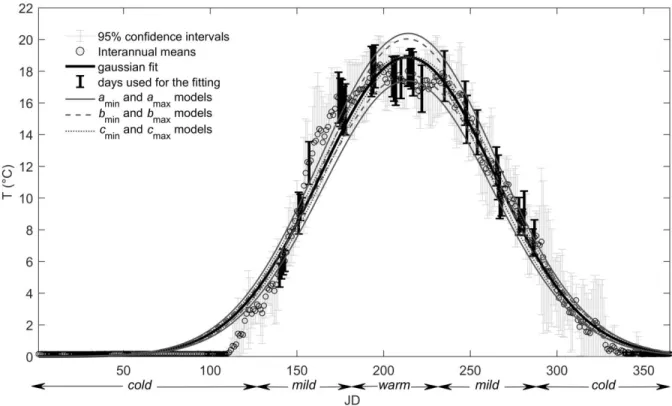
The Gaussian function is then fitted on 𝑇𝑤(𝑑) time series: 𝑇̂𝑤 ̅̅̅̅(𝑑) = 𝑎 exp (−1 2( 𝑑−𝑐 𝑏 ) 2 ) (6)

where 𝑇̂𝑤̿̿̿̿(𝑑) is the estimated interannual daily mean water temperature, a is scale parameter corresponding to maximum annual temperature, b, the standard deviation, is a measure of the duration of the warm period and c, the mean, is the date of occurrence of the annual maximum.

Confidence intervals on all three parameters can be estimated by fitting Equation (6) on limit values of daily means originating from the best datasets from each of the subsets corresponding to cold, warm and hot periods of the year (Erreur ! Source du renvoi introuvable.).

Figure 1. Gaussian functions fitted to daily interannual mean water temperatures to estimate the uncertainty of parameters a, b and c (from Daigle, Boyer, and St-Hilaire (2019)).

Two other metrics were used in the present study:

 MeanWaterTmax : Interannual mean of maximum temperature;

 MaxNumDay: Interannual mean of the number of consecutive days with maximum water temperature > 25 °C and minimum water temperature > 20 °C.

1. Identify days with Tmax > 95th _{annual percentile.}

2. Identify the earliest date (date_min) and the latest date (date_max) of days for which criterion 1 was met.

3. Count the number of dates between date_min-5 and date_max+5.

4. If the time series between date_min-5 and date_max+5 have fewer than 10% missing data, identify and maximum value in use it to calculate the interannual mean.

MaxNumDay :

1. Identify days for which Tmin > 20°C and Tmax > 25°C 2. Implement the procedure in steps 2 to 4 for MeanWaterTmax.

It should be noted that for nine stations, the number of years for which these metrics could be calculated were less than 3 and for one of these stations (Salmon River near Glenwood), this number was 0, because of the large amount of missing data in the period of interest.

3.1.3. Results

As described in the Methods section, the MLR and GAM models were tested for three different groupings: 1) all stations together; 2) HCA; 3) ROI. In each case, predictor selection was based on a stepwise approach, i.e. introducing predictors in the model incrementally to see if they improved the model. The number of stations varies with the different grouping methods. Table 1 lists the dependant variables selected for both MLR and GAM when all stations were grouped together. At least one air temperature variable (MeanAirTmax, MeanAirTmin) was selected for four out of five thermal metrics in the case of MLR and for three out of five metrics in the case of GAM. When no air temperature metric was selected, elevation or YCentroid, which are highly correlated with air temperature, were selected as predictors. River slope, basin area, forest cover and areal cover of grassland were also frequently selected.

Table 1. Selected predictors when all stations were grouped together.

Metric Explanatory variables

MLR

MeanWaterTmax MeanAirTmax Slope Shrubland Forest MaxElevation GlacialDeposits

MaxNumDay MeanAirTmax Slope MinAirTmin MeanAirTmin YCentroid Rock

Gaussian_a MeanAirTmax Slope GlacialDeposits Shrubland Forest MinAirTmin

Gaussian_b MeanAirTmin XCentroid BasinArea Forest Slope YCentroid

Gaussian_c YCentroid MinElevation MaxElevation Forest XCentroid TotPrecip

GAM

MeanWaterTmax YCentroid BasinArea Forest Grassland MeanAirTmax Rock

MaxNumDay YCentroid FluvioGlacialDeposits Grassland BasinArea Slope MeanElevation

Gaussian_a YCentroid Forest Grassland BasinArea Rock MeanAirTmax

Gaussian_b MinAirTmin MeanAirTmax Forest XCentroid Slope Wetland

Gaussian_c YCentroid BasinArea XCentroid Forest Slope ElevationStation

In the case of HCA, groups of stations were created depending on the cut-off threshold applied in the dendrogram. In order to select this level, various thresholds were used and performance metrics were compared. The cut-off threshold that yielded the lowest RMSE was selected. Figure 2 shows the dendrograms and selected thresholds for the GAM method for all five metrics. In all cases, the approach

yielded only two groups of stations. However, in the case of MLR (not shown here), three groups were created for MaxWater_Tmax and for Gaussian_a.

a)

c)

d)

Figure 2. Dendrograms with cut-off thresholds for a) MeanWaterTmax; b) Max_Num_Day; c) Gaussian_a; d) Gaussian_b; c) Gaussian_c. Note that not all station numbers are shown on the x-axis.

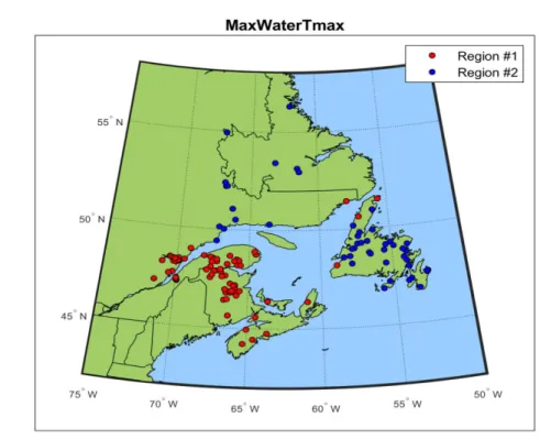
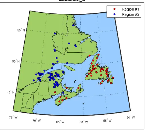
Figure 3 shows the regions created by the HCA approach. In most cases, one group mostly comprises stations located in the southwest portion of the study area, while the other occupies the northeastern part of the study area. However, it should be noted that there are exceptions. For instance, for MeanWaterTmax, three stations located in Newfoundland are associated with the group in red, for which the remainder of the station are mostly located in the southeastern part of the study region. For Max_Num_Days, some stations located near one another belong to two different groups.

a)

c)

e)

Figure 3. Maps of stations grouped using HCA-GAM for a) MeanWaterTmax; b) Max_Num_Day; c) Gaussian_a; d) Gaussian_b; c) Gaussian_c.

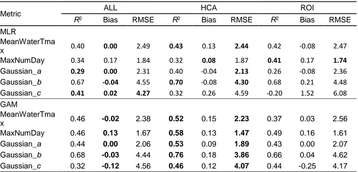
Table 1 lists the performance metrics for the different combinations of grouping methods and statistical models. It can be seen that in general, the GAM outperforms MLR. Also, HCA provides lower RMSE and higher R2 _{than ROI or using all stations together (ALL) in all cases when GAM is implemented. However,}

defining regions using HCA appears to yield slightly more bias than using a single region.

Table 2. Performance metrics for different Regional Thermal Analysis methods in Atlantic salmon rivers

Metric ALL HCA ROI

R2 _{Bias RMSE R}2 _{Bias RMSE R}2 _{Bias RMSE}

MLR MeanWaterTma x 0.40 0.00 2.49 0.43 0.13 2.44 0.42 -0.08 2.47 MaxNumDay 0.34 0.17 1.84 0.32 0.08 1.87 0.41 0.17 1.74 Gaussian_a 0.29 0.00 2.31 0.40 -0.04 2.13 0.26 -0.08 2.36 Gaussian_b 0.67 -0.04 4.55 0.70 -0.08 4.30 0.68 0.21 4.48 Gaussian_c 0.41 0.02 4.27 0.32 0.26 4.59 -0.20 1.52 6.08 GAM MeanWaterTma x 0.46 -0.02 2.38 0.52 0.15 2.23 0.37 0.03 2.56 MaxNumDay 0.46 0.13 1.67 0.58 0.13 1.47 0.49 0.16 1.61 Gaussian_a 0.44 0.00 2.06 0.53 0.09 1.89 0.43 0.00 2.07 Gaussian_b 0.68 -0.03 4.44 0.76 0.18 3.86 0.66 0.04 4.62 Gaussian_c 0.32 -0.12 4.56 0.46 0.12 4.07 0.44 -0.25 4.17 Scatter plots of observed vs simulated values are shown below for all models using leave-one-out cross-validation. These figures highlight the fact that in most cases, the bias is more pronounced for extreme (high or low) values of the temperature metrics than for central values. This is especially the case for MaxNumDay and Gaussian_c.

Figure 5. Scatter plots of observed vs. simulated values of temperature metrics for GAM.

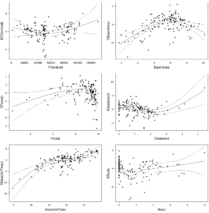
The GAM offers the potential advantage of having the capacity to model non-linear dependencies. As an example, Figure 6 shows the non-linear splines used to estimate Max_Water_Tmax for all the predictors used in the GAM model when all stations are included. Figure 6 shows the classical example of a flattening of the relationship between water and air temperatures for high values. It also shows that the relationship with drainage area follows a bell-shaped curve. This means that both low drainage area (i.e. low order streams) and high drainage area (i.e. deeper rivers with high flows) have cooler Max_Water_Tmax than medium size rivers with shallow water and open canopy.

Figure 6. Splines for the predictors used in the GAM-ALL model.

3.1.4 Conclusion

In this study, the analyses presented initially by Charron et al. (2019) were repeated using a database with a larger number of stations and fewer redundant information (i.e. fewer stations on the same river). Of the six candidate models, the one using HCA for grouping stations and GAM for metric estimation had the best performance, as in the case of Charron et al. (2019). The increase in the number of stations was made possible by relaxing the criterion related to the length of the time series, from five to four years. This resulted in slightly higher RMSEs and lower coefficient of determination in the present study, compared to the first one. However, results are still promising, especially for the first two parameters of the Gaussian function. Gaussian_a has a RMSE < 2°C and Gaussian_b has a RMSE < 4 days. Gaussian_c, which represents the mean temperature, has a larger RMSE (around 4 °C).

As in the first study, the HCA best model comprises only two regions when the GAM is used to estimate the temperature metrics. This relatively low number of regions may be caused by the fact that large sample sizes are required to adequately fit a GAM model. When the MLR model is used, three regions were identified for some of the metrics. As the database increases, these analyses will need to be revisited and it is anticipated that the large regions presented in this study will be further divided in sub-regions. Other recommendations include testing other grouping methods (e.g. Canonical Correlation Analysis used by

Guillemette et al. 2011) and other models such as multivariate adaptive regression splines (e.g. Lewis and Ray 1993). In spite of the fact that the current regionalization tool can be improved, it is now possible to provide first estimates of the metrics presented in this report on all Atlantic salmon rivers. This first estimation could provide important insight to managers on the thermal regime of rivers for which no or few data exist. It is also recommended that other temperature metrics be included in future analyses. They could include growth index, stress-inducing and lethal thermal thresholds, etc.

3.1.5 References

Boyer, Claudine, Andre St-Hilaire, R. Allen Curry, Daniel Caissie, and Gillis, Carole-Anne. 2016. “Technical Report: RivTemp: A Water Temperature Network for Atlantic Salmon Rivers in Eastern Canada.” Water News, Canadian Water Association Newsletter, Spring edition. Burn, Donald H. 1990. “An Appraisal of the ‘Region of Influence’ Approach to Flood Frequency

Analysis.” Hydrological Sciences Journal 35 (2): 149–65. https://doi.org/10.1080/02626669009492415.

Charron, Christian, Claudine Boyer, Andre St-Hilaire, Taha B. M. J. Ouarda, Anik Daigle, and Normand E. Bergeron. 2019. “REGIONAL ANALYSIS AND MODELLING OF WATER

TEMPERATURE METRICS FOR ATLANTIC SALMON (SALMO SALAR) IN EASTERN CANADA FINAL REPOR.” INRS Scientific Report #1855, 29 pages.

Daigle, Anik, Claudine Boyer, and André St-Hilaire. 2019. “A Standardized Characterization of River Thermal Regimes in Québec (Canada).” Journal of Hydrology 577 (October): 123963. https://doi.org/10.1016/j.jhydrol.2019.123963.

Guillemette, N., A. St-Hilaire, T. B. M. J. Ouarda, and N. Bergeron. 2011. “Statistical Tools for Thermal Regime Characterization at Segment River Scale: Case Study of the Ste-Marguerite River.” River

Research and Applications 27 (8): 1058–71. https://doi.org/10.1002/rra.1411.

Lewis, Peter A W, and Bonnie K Ray. 1993. “NONLINEAR MODELING OF MULTIVARIATE AND CATEGORICAL TIME SERIES USING MULTIVARIATE ADAPTIVE REGRESSION SPLINES.” In Dimension Estimation and Models, by Howell Tong, 136–69. WORLD SCIENTIFIC. https://doi.org/10.1142/9789814317382_0003.

McCullagh, P., and John A. Nelder. 1998. Generalized Linear Models. 2nd ed. Monographs on Statistics and Applied Probability 37. Boca Raton: Chapman & Hall/CRC.

4. Anticipated Risks

The work presented herein is mostly based on data from the RivTemp database (Boyer et al. 2016). RivTemp was established through a collaborative effort of a number of universities, government agencies and NGOs. The database is currently housed and managed at INRS. However, given the expansion of this network in recent years, it is becoming more and more difficult for the researchers involved to adequately fund the work required to coordinate and manage the monitoring, QA/QC and data storage required in RivTemp. If an alternative structure is not developed soon, there is a risk that the RivTemp database will no longer be managed to the level required for high quality data dissemination. A cooperative structure, whereby all key stakeholder provide not only data, but also financial resources to ensure proper coordination and data management/control, is an option that should be entertained in the near future.

5. Data Dissemination

The water temperature data used in this project were extracted from the RivTemp database. These data are already accessible via the RivTemp web site (www.rivtemp.ca). In addition, physiographic and meteorological data were used to define homogenous thermal regions. The physiographic data originate from different public sources (e.g. the Geological Survey of Canada and the Consortium for Spatial Information (CGIAR-CSI) and databases from provincial departments of natural resources). The meteorological data used in the study are daily air temperature and precipitation measurements interpolated on a 10km x 10km grid (ANUSPLIN; Hutchinson et al. 2009), which are also available online.

6. Publications

Charron, Christian, Claudine Boyer, Andre St-Hilaire, Taha B. M. J. Ouarda, Anik Daigle, and Normand E. Bergeron. 2019. “REGIONAL ANALYSIS AND MODELLING OF WATER

TEMPERATURE METRICS FOR ATLANTIC SALMON (SALMO SALAR) IN EASTERN CANADA.” INRS Scientific Report #1855, 29 pages.

St-Hilaire, A., T.B.M.J. Ouarda, C. Charron, C. Boyer, A. Daigle, N.E. Bergeron. 2019. Regional analysis of water temperature for the estimation of thermal indices at ungauged sites. AGU Fall Meeting, San-Francisco, November 2019

7. Statement of Accounts

The statement of accounts will be completed and provided by Ms. Marie-Noëlle Ouellet, one of INRS-ETE’s administrators.