THÈSE
En vue de l’obtention du
DOCTORAT DE L’UNIVERSITÉ DE TOULOUSE
Délivré par l'Université Toulouse 3 - Paul Sabatier
Cotutelle internationale : National Taiwan University
Présentée et soutenue par
Wei-Lin TU
Le 21 septembre 2018
Théorie de champ moyen renormalisée appliquée aux
matériaux quantiques avancés
Ecole doctorale : SDM - SCIENCES DE LA MATIERE - Toulouse Spécialité : Physique
Unité de recherche :
LPT-IRSAMC - Laboratoire de Physique Théorique
Thèse dirigée par
Didier POILBLANC
Jury
M. Nicolas REGNAULT, Rapporteur M. Chung-Yu MOU, Rapporteur M. Chung-Hou CHUNG, Rapporteur Mme Pina ROMANIELLO, Examinateur
M. Sung-Po CHAO, Examinateur M. Lei YIN, Examinateur
M. Didier POILBLANC, Directeur de thèse M. Ting-Kuo LEE, Co-directeur de thèse
Publication Index
[1] W. Tu and T.K. Lee, “Genesis of charge orders in high temperature
superconductors”, Scientific Reports 6, 18675 (2016)
Journal: Scientific Reports, Impact factor: 4.259
[2] P. Choubey, W. Tu, T.K. Lee, and P.J. Hirschfeld, “Incommensurate
charge ordered states in the t-t’-J model”, New Journal Physics 19,
013028 (2017)
Journal: New Journal Physics, Impact factor: 3.786
[3] W. Tu, F. Schindler, T. Neupert, and D. Poilblanc, “Competing orders
in the Hofstadter t-J model”, Physical Review B 97, 035154 (2018)
Journal: Physical Review B, Impact factor: 3.836
[4] W. Tu and T.K. Lee, “Pair density waves in the pseudogap phase of
cuprate superconductors”, manuscript under consideration by Scientific
Reports
Acknowledgements
To finish a thesis co-advised by two parties is not a easy task. I can never accomplish this without being helped by a lot of people. Among them, first, I need to show my 100 percent gratitude to Dr. T.K. Lee, who granted me this opportunity of conducting research under his supervision. Besides the knowledge I have learned and the training I obtained, the most important spirits I learned from him are the integrity and diligence that a scientist should possess. After occupying a same position and doing the same job for a long time, it is easy for a person to feel exhausted and therefore lose interest. But as a scientist it is a sign of danger because what we are doing for lifetime is the pursuit for the truth and reality. That can be the burden but also the joy. In these days collaborating with Dr. Lee, despite the hard time when we tried to settle down on the same page, I have never saw him lose interest in Physics. Considering how busy he is with also a administrative position as the director of Institute of Physics, Academia Sinica, this is even more difficult to keep the passion like he does. Those spirits I learned from him will be my lifetime treasure no matter if I succeed in becoming a scholar in the future.
Second, Dr. Didier Poilblanc also taught me a lot. The academic environ-ment in Taiwan is not that open compared with Europe where scientists from difference countries can easily meet each other. Thanks for his acceptance of my request of a joint-degree thesis, I got the chance to conduct research in France and therefore obtained many opportunities discussing physical topics with other outstanding scientists. To learn how to express my idea properly
is crucial in becoming an independent physicist and during the time in France those are among all what I got to learn the most. I think it is fair to say that he led me on the track of becoming an independent researcher from just a ap-prentice of physics. Thus, I want to thank Didier for not only teaching me a lot of academic knowledge, but also those chances he granted me for interacting with other experts in this field.
Plus, our co-workers mean a lot to me since they were willing to spare time collaborating with us upon certain issues. I would like to thank Dr. Peayush Choubey and Dr. Peter J. Hirschfeld from the University of Florida for participating in the work of analyzing STS results in detail with Wannier function. Dr. Peng-Jen Chen in Institute of Physics, Academia Sinica helped a lot for providing the Wannier90 package, too. Mr. Frank Schindler and Dr. Titus Neupert from the University of Zurich worked with us and provided their beautiful ED results and together we made a nice publication on Phys-ical Review B. Dr. Kenji Harada from the Kyoto University granted me the chance to start a short-term project with him which will become a very useful experience for my career.
As mentioned, to accomplish a co-advised degree is difficult and I cannot go through the administrative process with the help of secretaries from each parties. Therefore I need to thank the secretaries from TK group, Vicky Chen and Judy Hong, and from Department of Physics, NTU, Mr. Jih and Miss Lin. Also Malika Bentour from IRSAMC who provided me a lot of help not only during the administrative process but also for me better fitting in the life in France should be mentioned especially.
Also I want to thank my jury members, Dr. Nicolas Regnault, Dr. Pina Romaniello, Dr. Sung-Po Chao, and Dr. Lei Yin for accepting my request of being included in my committee. I cannot appreciate more for their time and energies spent upon me, a student they maybe never heard of before. Espe-cially, Dr. Chung-Yu Mou and Dr. Nicolas Regnault are also my responsible
referees who provided their reports to École Doctorale Science de la Matière for my thesis. I would like to thank for their extra effort for me.
Next, all my friends from TK group and Laboratoire de Physique Théorique should be mentioned too. Members from TK group no matter those who al-ready left or still with us provided me help and useful information from time to time. Those routine lunch time became more interesting with your com-panions. This is also the same for my colleagues in LPT. They helped me adjust myself for the life style in France. Thanks to them I no longer felt alone during the time in abroad. Especially, I would like to thank Mr. Huan-Kuang Wu and Dr. Giuseppe Alberti for kindly sharing their experience of preparing a defense.
At last, I need to show my gratitude to my family, my parents Jyy-Jiun Duh and Li-Ching Huang and my sister Jia-Jien Tu, and my girlfriend, Moeka Yamaguchi who we met in France. I would like to thank for your supports during my difficult moments. I want to share the glory, if there is any, to each of you.
Abstract
This thesis is aiming in utilizing the strongly correlated t− J Hamilto-nian for better understanding the microscopic pictures of certain condensed matter scenario. One of the long existing issues in the Hubbard model and its extreme version, t − J model, lies in the fact that there is not an analytical way of solving them. Therefore, when dealing with these models, numerical approaches become very crucial. In this thesis, we will present one of the methods called renormalized mean-field theory(RMFT) and exploit it upon the t− J model. Thanks to the concept proposed by Gutzwiller, all we have to do is to try to include the correlation of electrons, which is mainly the most difficult part, with several renormalization factors. After obtaining the correct form of these factors, we can apply the routine mean-field theory in solving for the Hamiltonian, which is the principle methodology throughout this thesis.
Next, the physical systems that we are interested in consist of two parts. The mystery of High-Tc superconductivity comes first. After 30 years of its discovery, people still cannot settle down a complete microscopic theory in describing this exotic phenomenon. However, with more and more experi-mental equipment with higher accuracy nowadays, lots of behavior of copper-oxide superconductor(also known as cuprate) have been revealed. Those dis-coveries can definitely help us better understand its microscopic mechanism. Therefore, from the theoretical side, to compare the calculated data with ex-periments leads us to know whether our theory is on the right track or not.
We have produced tons of data and made a decent comparison which will be shown in the main text.
The second system we are curious about is the mechanism of electrons under magnetic field. The Hofstadter butterfly along with its Hamiltonian, the Harper-Hofstadter model has achieved great success in describing free electrons’ movement with lattice present. Thus, it will be also interesting to ask the question: what will happen if the electrons are correlated. Our RMFT for t− J Hamiltonian, by adding an additional phase in the hopping term, happens to serve as a great preliminary model for answering this question. We will compare the results of ours with our collaborators, who solved this model by a different approach, the exact diagonalization(ED). Together with our calculations, we proposed several discoveries which might be realized by the cold atom experiments in the future.
摘要
本篇論文致力於使用強關聯電子模型之 t− J 漢密頓量來了解物質 之微觀行為,關於解釋強關聯之哈伯模型與其之極限對應的 t− J 模型 有一長久以為無法解決的問題為,我們無法用解析解完美詮釋此量子 模型;因此,在探討此模型時數值解便變得極為重要,在此篇論文中, 我們利用重整化平均場論近似 (RMFT) 之數值理論來探討 t− J 模型的 可能詮釋,歸功於 Gutzwiller 的發現,我們將可以把此模型中最困難 之部分:電子的強關聯性重整化為係數置於模型前,在得到這些相關 係數後,我們將可以利用平均場論的方法來對角化此一模型以便取得 其本徵函數,此一方法為此一論文之標準方法。 接下來,我們關心的物理情境分為兩大類,第一類為高溫超導體之 研究;在其最初發現於 1987 年以來已經過了 30 年,但科學家們仍無 法為其定調,但隨著實驗器具的精準度上升,我們越來越能清楚得知 其在微觀下的表現,這有助於幫助理論學家針對其建立一完整模型, 但同時也增加其困難因為要預想一合理之模型能夠完整解釋所有實驗 驗結果並非易事;我們的計算結果取得了許多數據,一一與實驗對比 的結果發現兩者之契合度非常之高,這也是我們對此模型抱有高度信 心之原因,詳細的比較結果將會在文中一一詳列。 第二類我們感興趣之系統為電子在強磁場作用之下的運動,霍夫斯 塔德蝴蝶與哈伯-霍夫斯塔德模型在自由電子於強磁場下在晶格內之運 動給了一完整描述,因此,探討同樣之運動唯電子具有關聯性便成為 一有趣課題,而我們的 t− J 模型在動能項增加一相位後,便成為一個 用來探討此物理情境的可靠模型;在此一研究之中,為了能更好得比較計算結果,我們的合作者採用了另一數值方法:完整對角化,我們 將會比較這兩種方法所計算出之結果並強調其可驗證性於未來之冷原 子實驗中。
Résumé
Cette thèse vise à utiliser le t − J Hamiltonian de la corrélation forte pour mieux comprendre la micro-fonctionnalité des scénarios de matériau condensé. Un des problèmes qui existe depuis longtemps est que pour ce type de modèle comme Hubbard Hamiltonian ou t − J Hamiltonian avec une corrélation forte ne peut pas être résolu complètement analytiquement. Par conséquent, quand on aborde ces modèles, il est important de les ex-ploiter de façon numérique. Dans cette thése, nous utiliserons la manière qui s’appelle “Renormalized Mean-Field Theory”(RMFT) pour le t− J Hamil-tonian. Grâce à M. Gutzwiller, ce que nous devons faire est simplement de chiffrer des paramètres qui incluent l’influence de la corrélation électronique et de les mettre avant chaque partie du Hamiltonian. Après ce calcul, nous calculerons l’Hamiltonian du champ moyen de manière standard. Ceci sera notre façon principale pour aborder des questions physiques.
Ensuite, nous l’appliquerons sur deux systèmes. Le premier est la mys-tique de supraconducteur à haute température. Après sa découverte il y a 30 ans, on ne peut pas encore définir une théorie pour expliquer sa micro-mécanique de manière appropriée. Cependant, avec des équipements avancés, on peut faire des expériences correctement et obtenir des résultats exacts. Ces preuves nous facilitent l’élaboration d’une bonne théorie, même s’il est aussi très difficile d’inclure tous les phénomènes ensemble. Nous avons obtenu des résultats et par rapport aux expériences, ils sont similaires qualitativement. Nous montrerons les détails dans le texte.
Le deuxième système qui nous intéresse est le mouvement d’électron dans un champ magnétique fort. Le papillon d’Hofstadter et son modèle, l’Hamiltonian de Harper-Hofstadter ont obtenu un grand succès à décrire la mécanique d’électrons libres aux treillis. Donc il est ainsi intéressant de se demander ce qu’il se passera si nous remplaçons des électrons libres avec ceux qui s’interagissent. D’ailleurs, t− J Hamiltonian s’utilise comme bon modèle à le découvrir. Nous allons comparer nos résultats avec ceux de la diagonalisation exacte. Nous proposerons des découvertes intéressantes qui désormais seront réalisées par l’expérience d’atome froide.
List of Abbreviations
ABS – Andreev Bound State AF – Antiferromagnetic AP – Anti-Phase
AP-CDW – Anti-Phase Charge Density Wave
ARPES – Angle Resolved Photoemission Spectroscopy ASH – Anderson, Shastry, and Hristopoulos
BdG – Bogoliubov-deGenne BZ – Brillouin Zone
CB – Checkerboard
CDW – Charge Density Wave CFP – Commensurate Flux Phase DC – Discommensurate
DOS – Density Of State DW – Density Wave
dSC – d-Wave Superconductivity
dSC-AFM – d-Wave Superconductivity+Antiferromagnetism ED – Exact Diagonalization
EDC – Energy Distribution Curve FQH – Fractional Quantum Hall FLS – Fermi Liquid State
FT – Fourier Transform GS – Ground State
GSD – Ground State Degeneracy GWA – Gutzwiller Approximation IP – In Phase
IPDW – Incommensurate Pair Density Wave iPEPS – infinite Projected Entangled-Pair State LDOS – Local Density Of State
nPDW – nodal Pair Density Wave PDW – Pair Density Wave
PG – Pseudo-gap
QI-APCDW – Quasi-Incommensurate Anti-Phase Charge Density Wave RVB – Resonate Valence Bond
RMFT – Renormalized Mean-Field Theory SC – Superconductivity or Staggered Current SDW – Spin Density Wave
STS – Scanning Tunneling Spectroscopy UPOP – Uniform Pairing Order Parameter
Contents
Acknowledgements v Abstract ix 摘要 xi Résumé xiii List of Abbreviations xv 1 Introduction 11.1 High-Tccopper oxide superconductivity . . . 1
1.1.1 The density waves . . . 3
1.1.2 The pseudo-gap phase . . . 7
1.2 Correlated electrons under strong magnetic field . . . 11
2 Renormalized Mean Field Theory 15 2.1 BdG equation of mean-field Hamiltonian . . . 15
2.2 Green’s function and LDOS . . . 20
2.3 Spectra weight and many-body Chern number . . . 24
3 Results I – High TcCuprate 27 3.1 Real space properties . . . 27
3.1.1 Charge-ordered patterns . . . 27
3.1.3 Bias and doping dependence . . . 37
3.1.4 Discussion . . . 41
3.2 Momentum space properties . . . 42
3.2.1 Particle-hole asymmetry . . . 43
3.2.2 Two-gap in the SC phase . . . 45
3.2.3 Finite temperature IPDW states . . . 47
3.2.4 Discussion . . . 52
3.3 Some details . . . 55
3.3.1 Method to determine kG . . . 55
3.3.2 Two-gap plots . . . 56
3.3.3 Choices of Γ . . . 57
3.3.4 Fermi arcs and LDOS . . . 58
4 Results II – Correlated Electrons Under Magnetic Field 61 4.1 Uniform and modulated singlet flux phase . . . 62
4.2 Fully polarized electron systems . . . 68
4.3 Topological properties . . . 69
5 Conclusions and Outlooks 73 6 Sommaire 79 6.1 Méthode . . . 79
6.1.1 Équation BdG de Hamiltonian du champ moyen . . . 79
6.1.2 Fonctions de Green et LDOS . . . 85
6.1.3 La spectre et le nombre de Chern . . . 88
6.2 Supraconduteur à haute température . . . 89
6.2.1 Charactéristique en éspace réel . . . 89
6.2.2 Charactéristique en éspace d’élan . . . 90
6.3 Électrons corrélé dans un champ magnétique . . . 93
A Exact Diagonalization 119
A.1 Model . . . 119 A.2 Many-body Chern number . . . 119 A.3 Results . . . 122
List of Figures
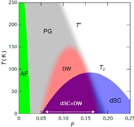
1.1 The phase diagram of hole-doped cuprate. The vertical axis is the tem-perature in the unit of Kelvin and the horizontal axis is the hole doping level. T∗ is the transition temperature of pesudo-gap phase, marked by PG while Tcis the one for d-wave superconductivity, marked by dSC. AF
stands for the phase of antiferromagnetism and DW pins out the region where density wave appears. The detailed discussion of each phase is in the text and this figure is borrowed from Ref. [1] . . . 3
2.1 Distribution of the phases ϕij on the bonds of 4×4 and 2×2 unit cells (on
the 2-torus) for the flux densities Φ considered in this work(times π/32). Arrows again indicate the directions of current and negative signs stand for opposite flows. The flux density Φ = 1/4 has only two different bonds (bond 1 and 2). The right panel shows detailed numbers of variables for the patterns we have obtained. Those patterns will be discussed later. . . . 17
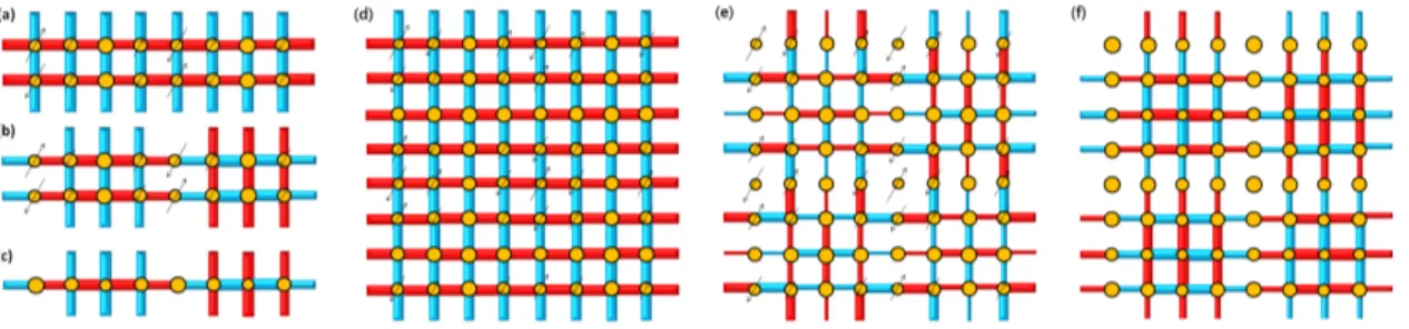
3.1 Schematic illustration of modulations for stripe like patterns. (a) IP-CDW-SDW (b) AP-CDWIP-CDW-SDW (c) AP-CDW (d) IP-cCB-sCB (e) AP-cCB-sCB (f) AP-cCB respectively. Size of the circle represents the hole density. The width of the bond around each site represents the amplitude of pairing ∆(∆ = ∑µ∆µ) and sign is positive (negative) for red (cyan). The size
of black arrows represents the spin moment. The average hole density is about 0.1 but 0.09 for IP-cCB-sCB. . . 28
3.2 (a) Energy per site as a function of hole concentration. Six states are shown in the main figure with notations defined in Table 2. The lower (upper) inset is for stripe (CB) patterns. Blue triangles, circles, and diamonds are for IP-CDW-SDW, AP-CDW-SDW, and AP-CDW respectively. And red triangles, circles and diamonds are for IP-cCB-sCB, AP-cCB-sCB, and AP-cCB respectively. (b) Schematic illustration of modulations for nPDW stripe. The numbers in red denote the hole density at each site while the numbers in black below them represent the pairing amplitude in y direction. The rest numbers above the figure stand for the pairing amplitude in x direction. Here our pairing amplitudes denote (⟨ci↑cj↓⟩).
Note that in this figure neither the size of circles nor the width of bonds represent amplitudes. The hole concentration is 0.125. (c) LDOS at 8 sites plotted from energy 0.6t to -0.6t. The inset shows hole density along the modulation direction of the nPDW stripe and (d) from 0.2t to -0.2t but shifted vertically for clarity. . . 29
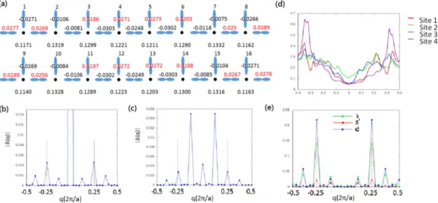
3.3 Properties of nPDW. (a) The real space modulation of nPDW in 32×32 lattice sites with δ= 0.125. Since the pattern repeats itself with an inversion symmetry in the middle bond, here we only show the first 16 sites. The red and black numbers on each bond denote the values of pairing order and the number at each site(black dots) is the hole density. (b)(c) The Fourier transform of the value of hole density(b) and pairing order(c). (d) LDOS of the first 4 sites of this 32×32 nPDW. (e) Different form factors. . . 32
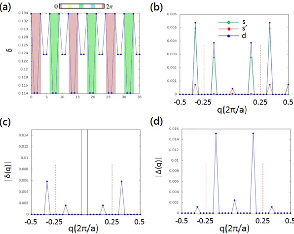
3.4 Figures showing the properties of discommensurate nPDW. (a) The phase variation of this pattern. Site 0-3, 12-15, and 24-27 are of phase equal to 0(2π) while sites 6-9, 18-21, and 30-33 are of phase π. (b) Form factors for discommensurate nPDW. We also include the Fourier transform of hole density(c) and pairing order(d). . . 33
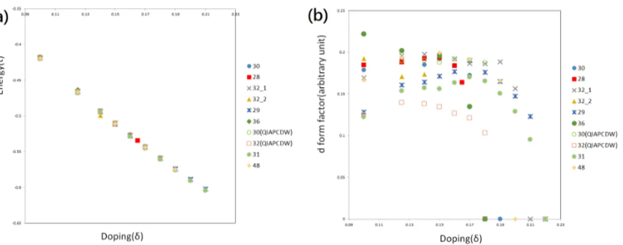
3.5 (a) Energies of several states chosen by us. Although we have listed ten different states here, their energies seem to be nearly degenerate and fol-low the same trend line. (b) Magnitude of d form factor of patterns. Given different states we expect their magnitude to change but still all of them seem to have the same trend: the magnitude maintains the same until dop-ing level exceeds 0.18, where it starts to drop drastically and becomes zero in the range of 0.18∼0.22. . . 34
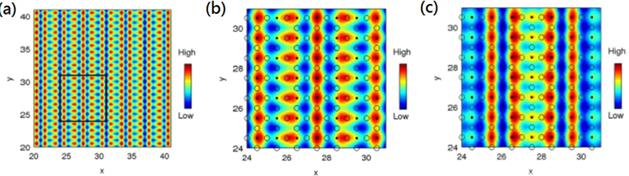
3.6 Continuum LDOS map at ω = ±0.25t and ∼ 5 angstrom above BiO
plane. (a) LDOS map at ω = 0.25t in a range of 20×20 unit cells located in the central region of 60×60 lattice. (b) Zoomed-in view of the area marked by square in (a). Black dots and open circles represent positions of Cu and O atoms, respectively, in the CuO plane underneath. (c) LDOS map at ω =−0.25t in the same region as in (b). . . 36 3.7 Continuum LDOS spectrum registered above Cu, Ox and Oy sites in the
unit cell (25, 25) at an height∼ 5 angstrom above BiO plane (a)without, and (b)with Γ = α|ω| inelastic scattering (α = 0.25), as extracted in [2]. The location of the unit cell can be referred from figure 4(b) as shown in the inset. Dots and open circles represent Cu and O atoms, respectively. . 37 3.8 (a) Bias dependence of the intra-unit cell form factors at x = 0.125
com-puted from atomic sublattice averages as described in the text.Next to it are the doping dependence of (a) energy at which d-form factor peaks (Ωd)
and (b) corresponding magnitude (DmaxZ ). . . 38
3.9 (a) Bias dependence of average spatial phase difference defined in equa-tion (18). (b) Bias Ωp at which initial π phase jump in ∆π takes place
versus doping. (c) Lattice LDOS in the case when nPDW charge and bond modulations are turned off keeping only pair field modulations. (d) Lattice LDOS in the case when nPDW pair field modulations are turned off keeping charge and bond modulations. . . 39
3.10 (a) and (c) Form factors and average spatial phase difference(∆ϕ) in the case when nPDW charge and bond modulations are turned off keeping only pair field modulations. (b) and (d) Form factors and average spatial phase difference (∆ϕ), respectively, in the case when nPDW pair field modulations are turned off keeping charge and bond modulations. . . 40
3.11 The quasiparticle spectra of a nPDW state calculated in a 32×32 lattice for hole concentration 0.125: (a) the vertical cuts (V 1-V 5) denote the y component of the momentums scanned from (b)(near nodal region) to (f)(anti-nodal region). (b)-(f): quasiparticle spectra weight for each cut as a function of ky with a fixed kxvalue shown above each figure. . . 43
3.12 The quasiparticle spectra of a nPDW state calculated in a 32×32 lattice for hole concentration 0.125: (a) the vertical cuts (H1-H5) denote the y component of the momentums scanned from (b)(near nodal region) to (f)(anti-nodal region). (b)-(f): quasiparticle spectra weight for each cut as a function of kxwith a fixed ky value shown above each figure. . . 44
3.13 The gap value evolving from nodal to antinodal region for nPDW for (a) two different lattice sizes at doping 0.125; (b) different doping levels but same size(30×30). Red, green and purple lines are just guides for the eyes. The black dotted(dashed) line is a plotted pure d-wave(antinodal) gap with gap size about 0.075∼ 0.08t(0.2t). . . 46
3.14 UPOP vs temperature for δ= 0.125, 0.15, and 0.16. Tp1and Tp2 for each
case are marked with different dotted lines of the same colors. The lattice size is 30×30. . . 48
3.15 Properties of IPDW. (a) The real space modulation of IPDW. The red and black numbers on each bond denote the values of pairing order and the number at each site (black dots) is the hole density. (b) The LDOS for sites near the domain wall(2, 6, 9, 14 in (a)) and in the middle of nearby domain walls(1, 4, 8, 15 in (a)). (c) Different form factors and (d)(e) Fourier transform of hole density(d) and pairing order(e). The red vertical dashed lines mark|q| = 0.5π/a corresponding to period 4a. Quasiparticle spectra with zero energy in k space for IPDW in 30×30 lattice sites at T = 0.035t are shown in (f) for δ = 0.15. The cyan dotted curve is the Fermi surface of Fermi liquid state with the same doping level. Γ used here is equal to 0.25√E2 + T2[2]. . . . 49
3.16 (a) Doping dependence of Tp1and Tp2. Tp1/2 and Tp2/2 are shown with
the blue triangles and diamonds respectively. The results from NMR [3] are also shown for comparison. We choose 0.1t ∼ 464 K. (b) The gap values scanned along the Fermi surface at T = 0 and 2Tp1 for δ =
0.15. (c) Doping dependence of the relative DOS between IPDW and FLS(DOSIP DW/DOSF LS) at T = 0.035t. The experimental data from
[3] for T = 0 is also plotted for comparison. The inset shows DOS of IPDW vs temperature for δ = 0.125, 0.15, and 0.16. Γ we used here is 0.25√E2+ T2 [2]. . . . 50
3.17 We list several quasi-particle spectra at antinodes((π, 0)/(0, π)) for three different patterns at different temperatures. Although marked as nPDW in the first column, the patterns become IPDW at T = 0.035t and T = 0.05t. However their spectra do not change much and the differences of gap values at (π, 0) and (0, π) are within 10% [4]. . . . 52
3.18 (a) A collection of several data points of kG− kF vs doping at kx = π.
The way of determining the difference of kG and kF is shown in (b): kG
determined by examining EDCs plotted from ky = 0 toward ky = pi,
for dopant concentration 0.15. kF is determined by Fermi liquid surface
and marked along with kG on the EDC plot. The quasiparticle spectra is
also shown with Gaussian width Γ = α|E| (α = 0.25) and marked with positions of kGand kF. . . 56
3.19 (a) Two-gap plot for nPDW at δ = 0.125 as shown in Fig. 3 in the main text but obtained from different approaches: red line is determined by the gap values shown by quasiparticle spectra but green line comes from EDCs. (b) Relative DOS as a function of hole concentration as in Fig. 3.16(c) in the main text but put together with two different Γ. The two blue lines are very close to each other. (c) Two gap plots determined by different Γ for nPDW at δ = 0.15. One can see that these lines nearly overlap with each other. Figure (d) and (e) again show the quasi-particle spectra for nPDW at δ = 0.125(for the 32× 32 lattice) at kx = 0.977π but
with different Γ: (d) Γ = 0.01t and (e) Γ = 0.25|E|. Note that in fact (d) is identical as Fig. 3.11(f) in the main text. We can find that although these two figures look quite different due to the choices of Γ, important features such as location of kGare still the same, only that in (e) the spectra bands
are broadened due to larger Γ. . . 57 3.20 (a) and (b) Zero energy quasiparticle spectra in k space before(a) and
af-ter(b) taking average of x- and y-directions PDW. (a) is the same as Fig. 3.15f and we put it here again for the reason of comparison. Clearly, (b) looks more like the observation by experimental groups. (c) and (d) LDOS at sites near(c) and away from(d) domain walls at different temperatures for nPDW(IPDW) at δ = 0.15. Γ used here is equal to α√E2+ T2(α = 0.25). All figures shown here are of 30× 30 lattice size. Its Tp1is around
4.1 “Phase diagram” vs electron filling ρ and magnetic flux Φ showing the various phases presented in Table 4.1. Circles are non-polarized (singlet) states while squares represent ferromagnets. Black symbols correspond to uniform solutions. Red, green, and blue symbols encode symmetry-breaking supercells of size 4× 4, √2×√2, and 2× 2 (with staggered potential for Φ = 1/4) respectively. . . 63
4.2 Comparison between RMFT and ED energies (per magnetic 4× 4 unit cell). (a) Kinetic energy and (b) magnetic (potential) energy vs inserted flux Φ. The doping level is fixed to δ = 1/8 and J = 0.3t. The numerical values are given in the Table 4.2. . . 65
4.3 Schematic patterns and results for the states in this subsection. (a)-(d) show the current and hopping patterns of each state within the 4× 4 sub-lattice. The widths of the underlying orange bars and black arrows rep-resent the magnitudes of hopping and current on each bond separately. The flows of current are indicated by the arrow directions. The numerical values are shown in Fig. 6.1. . . 67
4.4 Band structure for the three lowest energy bands for (a) ν∗ = 2/7 and (b) ν∗ = 2/5. At this doping, the first two bands are filled. Note that in (a) the first two bands are almost degenerate. . . 69
6.1 Distribution of the phases ϕij on the bonds of 4×4 and 2×2 unit cells (on
the 2-torus) for the flux densities Φ considered in this work(times π/32). Arrows again indicate the directions of current and negative signs stand for opposite flows. The flux density Φ = 1/4 has only two different bonds (bond 1 and 2). The right panel shows detailed numbers of variables for the patterns we have obtained. Those patterns will be discussed later. . . . 82
A.1 (a) Vector potential gauge choice for Φ = q/16, q = 0,· · · , 15. Periodic boundary conditions are assumed. Aij in units of F = 2πΦ is given by
the integer number shown between site i and j, with positive sign if the respective arrow points from site i to site j, and negative sign otherwise. (b) Spectrum E(ϕ) as a function of inserted flux for ν = 1/5. The Chern number evaluates to 6, however, there is no indication for a topological GSD. . . 120 A.2 Lanczos ED spectrum of H for various values of ν, with Φ and ρ as given
by Table A.1. When there is no magnetization, only the Sz = 0,±1 sector
is shown. . . 121 B.1 RMFT energy spectrum as a function of staggered potential δ with Chern
numbers for each band shown beside the figure. For Γ > 2t the system is topologically trivial with the Chern number C of the bands zero. At the transition point, the band gap closes and it becomes topologically non-trivial with C = 1 for the lowest band. After passing the transition point, the gap opens again and the lowest band now possesses a Chern number of -1. Notice that within this chosen reduced BZ, each of the four bands originating from the 2×2 modulation is folded into 4 sub-bands, producing a total of 16 bands. . . 125
List of Tables
3.1 Definition of various nearly degenerate states with respect to the inter-twined orders: pair field, charge density, and spin moment. Besides the two uniform solutions, d-wave superconducting(dSC) state and coexis-tent antiferromagnetic(dSC-AFM) state, all the states to be considered in this paper, unless specifically mentioned, have modulation period 4a0 for charge density and bond order. IP(AP) means the pair field is in-phase with period 4a0(anti-phase with period 8a0). IP has a net pairing order and AP has none. SDW is the spin density wave with period 8a0. sCB(cCB) denotes the checkerboard pattern of spin(charge) and diag means the di-agonal stripe which has in-phase pair field and spin modulation. . . 28
4.1 Parameter sets used in the following subsections. Ns, Ne, and NΦ are the site, electron and flux numbers used for performing RMFT (those for the ED on a 4× 4 cluster are obtained from a simple rescaling). Sets are listed with decreasing electron filling from top to bottom. The GS is either a singlet (S = 0) or fully polarized (FP), i.e., the total spin is S = Ne
2 (in that case ν∗ = 2ν is listed and marked with an asterisk). The supercell associated to a possible spontaneous (charge or bond) ordering
is also shown. 1×1 means the GS is uniform. CDW, BDW, and PDW
stand for charge, bond, and pairing density wave. SC means staggered current modulation. For ρ = 7/16 and Φ = 5/16 or 3/16, including (d-wave) superconducting order in addition to CDW/BDW order gives a PDW self-consistent solution with lower energy. For ρ = 1/8 and Φ = 1/4 (ν∗ = 1), the 2× 2 modulation is induced by a staggered potential. Otherwise, translation symmetry breaking (if any) occurs spontaneously. . 62 4.2 Table of the energies and Chern numbers for the self-consistent solutions
obtained in RMFT. E0 = Ekin + Epot represents the energy per 4× 4 sublattice. The last column is the Chern number given by summing up the contribution from all the filled (mean-field) bands. The last five rows noted by an asterisk represent the fully polarized states for which ν∗ = 2ν is listed instead of ν. . . . 64 4.3 Summary of the Lanczos exact diagonalization results. . . 66 4.4 Table comparing the Chern numbers obtained in the non-interacting case,
in the (non-superconducting) RMFT self-consistent solutions and by Lanc-zos ED. In the two first cases, the Chern numbers are given by summing up the contribution from all the filled bands. The last five rows noted by an asterisk represent the fully polarized states for which ν∗ = 2ν is listed instead of ν. . . . 70 A.1 Summary of the Lanczos exact diagonalization results. . . 121
Chapter 1
Introduction
This introduction is divided into two parts corresponding to two scenarios that we are going to talk about. The first part is for introducing the key issues that still exist and are unsolved to the physical society, which leave the problems of high-Tc superconductivity still in
the center of stage until now. We will first go through a review upon several important features of it and then bring up the questions that we want to resolve. And then it comes the second interesting system which is the physical system of placing interactive electrons within lattice under strong magnetic field. We will, starting from the initiative by D. R. Hofstadter, compare the calculations executed by two different methods to try to provide a clear picture of what is going to take place when such scenario arrives.
1.1
High-T
ccopper oxide superconductivity
The first discovery of such novel materials with such beautiful characteristic was in 1986 by Bednorz and Müller [5], who won the Nobel Prize in Physics with the Non-stoichiometric copper oxide(also referred to as cuprate), the Lanthanum barium copper oxide(La2−xBaxCuO4, LBCO) with transition temperature as high as 35 K, in the following year. After the first success, in the years of 1986 to 2008 lots of new cuprate materials were found in series. Among them, the most famous one goes to the yttrium barium copper oxide(Y Ba2Cu3O7, YBCO) discovered by Wu and Chu [6] in 1987. Other examples include the bismuth stron-tium calcium copper oxide(Bi2Sr2CanCun+1O2n+6−d, BSCCO) [7] with Tc= 95−107K
varying with the number of n, and thallium barium calcium copper oxide(T lmBa2Can−1CunO2n+m+2+δ, TBCCO) with highest possible Tcto be 127 K [8]. Until now, the highest transition
tem-perature confirmed is at 135 K observed in 1993 with the layered cuprate HgBa2Ca2Cu3O8+x [9] and when applied under pressure, its Tccan achieve above 150 K.
What was so exciting about the discovery of such high-Tccuprate lies on the fact that
it breaks the temperature limit set by Bardeen-Cooper-Schrieffer(BCS) theory that was proposed in 1957 [10]. In BCS theory, the phonon plays the role as the medium to com-bine two electrons, despite their repulsion, in momentum space. In such mechanism, the maximum transition temperature is around 23 K, which is way lower than any temperature at which a efficient industrial usage can be applied. However, the transition temperature of cuprate has surpassed the boiling point of liquid nitrogen, which is easily available nowadays.
Besides the practical application, the violation of the estimation by BCS theory also implies that the phonon interaction may not be enough to properly describe the micro-mechanism of high-Tcphenomena. Thus, one of the questions should be asked naturally
will be that what kind of interaction could sustain the electronic pairing stronger than the one mediated by phonon. To answer this, we need to sort out the features. First, we notice that in the phase diagram shown in Figure 1.1, the first appearing phase is the antifer-romagnetism(AF). In fact, when there is no doping of hole, the material itself is a Mott insulator [11], composed of the antiferromgnetic ordering and mottism, meaning that the material is an insulator due to the strong electron-electron repulsion. Upon doping, the mottism disappears along with its antiferromagnetic order, which matches the experimen-tal observation of cuprate.
What we want to ask next is the reason why superconductivity appears after the Mot-tness(antiferromagnetism+mottism) is suppressed by doping. P. W. Anderson was the first among all to propose a theoretical model named after the resonating valence bond theory(RVB) to try to explain the appearance of superconductivity after doping from a insight inspired by strong correlation [12]. In this theory two electrons from neighboring copper atoms tend to form a valence bond. These bonds will resonate within the Cu− O
Figure 1.1: The phase diagram of hole-doped cuprate. The vertical axis is the temperature in the unit of Kelvin and the horizontal axis is the hole doping level. T∗ is the transition temperature of pesudo-gap phase, marked by PG while Tcis the one for d-wave
supercon-ductivity, marked by dSC. AF stands for the phase of antiferromagnetism and DW pins out the region where density wave appears. The detailed discussion of each phase is in the text and this figure is borrowed from Ref. [1]
layer but without doping they cannot transfer in space. However, when vacancies appear with doping, they become mobile and result in the superconductivity. The principle mod-els for describing the RVB theory are the Hubbard and t− J models, and the later will be our central model for this thesis.
1.1.1
The density waves
Although the picture provided by Anderson seems to be quite clear and acceptable, the issue of high-Tc has not yet been settled down due to several reasons. One, the strong
correlated models are usually very difficult to obtain their exact solutions and, unfortu-nately, the Hubbard and t− J models are of this genre. Despite the effort by physicists
from numerical parts that provides many reliable calculations for these two models, we still need more proofs before making any further claim. Second, the existence of other un-usual phases in the phase diagram is also a pending issue to be explained. The first is the phase of density wave marked by DW in Figure 1.1. Ever since the discovery of the high-Tc superconductivity, many low-energy charge-ordered states in the cuprate have been
discovered. Neutron scattering experiments [13] first emphasized the doping dependence of incommensurate magnetic peaks associated with unidirectional magnetic patterns or stripes. Later, soft X-ray scattering [14] also confirmed the presence of charge orders with these stripes. However, these experiments were performed on the 214(La2−xSrxCuO4) cuprate family. For other cuprate families, the evidence for bond-centered unidirectional domains was found via scanning tunneling spectroscopy [15, 16]. The charge density wave(CDW) order was also found to be induced by the external magnetic field [17]. Re-cently, more results regrading charge-ordered states [18, 19, 20, 21, 22], and electron-doped cuprates [23] have been reported. The periods of these CDW and their doping dependence are quite different for different cuprate families [22]. In addition to the uni-directional stripe pattern, some experiments have also reported the possible existence of a bidirectional ordered checkerboard pattern [24, 25]. The unidirectional charge-ordered states or stripes were found to have a dominant d-like symmetry for the intra-unit-cell form factor, measured on the two oxygen sites by using the resonant elastic X-ray scattering method [26, 27] and via scanning tunneling spectroscopy(STS) [28]. However, different families seem to prefer different symmetries [26, 27]. In the STS experiments [29], the density waves disappeared above 19% hole doping. Furthermore, the observation of these CDW states having nodal-like local density of states(LDOS) at low energy but strong spatial variation at high energy in STS [15] strongly implies a new unconventional superconducting state.
The existence of these great varieties of charge-ordered states has created a great de-bate regarding whether the strong coupling Hubbard model or the t− J model [12] is the proper basic Hamiltonian to describe the cuprates. Many believe that these states “com-pete” with the superconductivity [30] and that their origin may reveal the fundamental
understanding of the mechanism of high superconducting temperatures in cuprates. The recent detection of the d-form factor at an oxygen site instead of at a Cu site [26, 27, 28] also raises the question about the suitability of the effective one-band Hubbard or t− J model and the validity of replacing the oxygen hole with a Zhang-Rice singlet [31], which effectively supports a simpler one-band model with Cu only. Allais et al. [32] proposed that the d-symmetry of these form factors, referred to as bond orders [33, 34] because they are measured between the nearest neighbor Cu bonds, arise from the strong correlation but without other intertwined orders. Furthermore, there are also doubts regarding whether a strong correlation is present or even needed to understand of the superconducting mech-anism [35]. However, the complexities of the phase diagram and some recent theoretical works have indicated the possibility of a new phase of matter, i.e., the pair density wave (PDW) [36, 37, 38, 39], as discussed in detail in a recent review article [36]. The new states are considered to have intertwined orders of PDW and CDW or spin density waves (SDW) [36]. Actually there are many different kinds of PDW states that could be either unidirectional [40] or bidirectional like a checkerboard. For the unidirectional PDW state intertwined with CDW and SDW, so called the stripe state, was first proposed by the vari-ational calculation for the t− J model [41]. It could have the same sign of d-wave pairing on each site or pairing is in-phase so that the period of modulation of pairing is same as charge density but only half of the SDW. Or it could be the anti-phase stripe having two domains with opposite pairing sign so that the period of pairing modulation is twice of the charge density. The in-phase stripe was later shown [42] to be a stable ground state with half a hole in each period of CDW when a small electron-phonon interaction is included in the t−J model. This half-doped stripe may be what was observed in neutron scattering [13] for the LBCO(La2−xBaxCuO4) family.
For quite some time, various calculations [40, 41, 42, 43, 44, 45, 46, 47, 48, 49, 50] on the Hubbard and t− J type models have revealed low-energy intertwined states ap-pearing as stripes or bidirectional charge-ordered states, such as checkerboard(CB). How-ever, these works usually involved different approximations and parameters, which often resulted in different types of charge-ordered patterns, and these studies were mostly
con-centrated at a hole concentration of 1/8, which is the most notable concentration in early experiments. Hence, it is not clear if these results were the consequence of the invoked assumption or the approximation used, or if they are a generic results in the phase dia-grams of cuprates. There were attempts to produce these CDWs or PDWs using a differ-ent approach, such as using a mean field theory to study a t− J-like model but taking the strong correlation as only a renormalization effect of dispersion [33, 34, 51, 52]. A spin-fluctuation mediated mechanism to produce these states was also proposed for the spin-fermion model [53]. Recently, a novel mechanism of PDW was proposed, i.e., Am-perean pairing [39], by using the gauge theory formulation of the resonating-valence-bond picture. In most of these approaches, the wave vectors or periods of the density waves are related to special features of the Fermi surface, including nesting, hot spots or regions with large density of states. However, the opposite doping dependence of CDW periods, observed for 214 and 123 (Y Ba2Cu3O6+δ) compounds [22], makes the Fermi surface scenario worrisome.
Amid all this confusion, recent numerical progress achieved by using the infinite pro-jected entangled-pair states(iPEPS) method [54], has provided us with a new clue. It was found that the t− J model has several stripe states, with nearly degenerate energy as the uniform state and, with coexistent superconductivity and antiferromagnetism. The period of the PDW moves toward 4 or 5 lattice spacing as U increases and this is more in line with result of the t− J model. When the number of variational parameters is extrapolated to infinity, the authors concluded that the anti-phase stripe, which has no net pairing, has slightly higher energy than the in-phase stripe with a net pairing, which in turn, also has slightly higher energy than the uniform state. The results are quite consistent with the most recent numerical studies on the Hubbard model [55]. They found the stripe states have lower energies than the uniform SC state at 1/8 hole density and for U = 8 and 12. These results are very consistent with the result of variational Monte Carlo calcula-tions [43] based on the concept of the RVB picture [12]. Furthermore, the results are also consistent with that of renormalized mean-field theory by using a generalised Gutzwiller approximation(GWA) [56] to treat the projection operator in the t− J model [40, 57].
Hence, the result provides strong support to more carefully examine the low energy states of the t− J model with the variational approach using GWA.
Among all the discoveries of different states, anti-phase charge density wave (AP-CDW) and nodal pair density waves (nPDW) have dominant d-form factor and exist in the doping range where charge order has been experimentally observed. The AP-CDW is a charge order with commensurate wave vector e.g. (0, 0.25π) or (0.25π, 0), that has been studied extensively in Ref. [40]. These states have an accompanying superconducting order parameter that forms domains with opposite signs (AP). The nPDW is an incom-mensurate charge order with wave vector (0, Q) or (Q, 0), where Q ∼ [0.25π, 0.3π]. In addition to the modulating component, the pair field has a uniform d-wave component giving rise to nodal structure in the density of states at low energies similar to the exper-imental observation [15]. Thus the nPDW intertwines uniform superconductivity, PDW and charge order. Capello et al. [58] have proposed such a state with an uniform pairing order but it is not a pure d-wave order. Instead of proposing a possible state by conjec-turing, we have solved a set of self-consistent equations derived from the RMFT. Of the many low energy solutions we found, nPDW explains a number of properties measured by the STS on BSCCO(Bi2Sr2CaCu2O8+x) and NaCCOC(Ca2−xN axCuO2Cl2) [59]. Its period of the CDW is about half of the PDW. Furthermore, by including the Wannier function in our calculation to take into account the effect of oxygens that were neglected in the simple t− J model, we are able to compute the continuum local density of states of the nPDW. The energy dependence of intra-unit cell form factors and spatial phase vari-ations of these states agrees remarkably well with the STS experiments [28, 59]. We will analyze them further in the following section.
1.1.2
The pseudo-gap phase
After demonstrating the appearance of DWs coming from the t− J Hamiltonian with our RMFT, we note that in Figure 1.1 the DW phase is always co-existing with the PG phase. So the next task is to check among those solutions we obtained if some of them are also able to contain the features of PG besides DW. A long standing unresolved puzzle of the
cuprate high temperature superconductors is the nature of PG phase [60, 61]. Below the PG temperature T∗there are experimental evidences of breaking some crystalline symme-try [62, 63]. Breaking of time-reversal symmesymme-try with observation of intra-cell magnetic moments has also been reported [64]. Many more new evidences suggest that this phase should be a nematic phase that breaks the four-fold rotation symmetry of the copper oxy-gen lattice [65, 66, 67]. In particular there are many reports of the CDW or SDW in the SC and PG phases [13, 14, 26, 68, 69]. Some of these are likely unidirectional hence without four-fold rotation symmetry. There are experimental evidences indicating the presence of fluctuating or short-range-ordered CDW in the PG phase [19, 26, 70]. Once the CDW sets in and breaks four-fold symmetry [15], the symmetry of pairing order in the SC phase of tetragonal crystal such as Bi2Sr2CaCu2O8+x should not be expected as a pure d-wave as seen in experiments [71, 72]. Thus the formation mechanism of these DWs and its relations with SC and PG phases are of great interests.
Before the discovery of these density wave orders in the cuprates, the PG phase has already posed a number of unexplained puzzles. Below a characteristic temperature T∗ but higher than the SC transition temperature Tc, the excitation spectra showing a gap
was first noticed by the relaxation rate of nuclear magnetic resonance [73] and then by many other transport and spectroscopic measurements [74]. But the most direct obser-vation of this gap structure was shown by the the angle-resolved photoemission spec-tra(ARPES) [75, 76, 77]. The energy-momentum structure shows an energy gap appears near the boundary, or the antinodal region, of the two-dimensional Brillouin zone(BZ) of the cuprate. However there are four disconnected segments of Fermi surface near the nodal region, or|kx| = |ky| = π/2. These segments called Fermi arcs have been
re-ported to have their length shrink to zero [78, 79] when extrapolated to zero temperature. There are also results indicating that the arc length is not sensitive to temperature [19, 76]. Then it could also be part of a small pocket [80, 81]. This presence of finite fraction of Fermi surface is consistent with the Knight shift measurement [3] showing a finite den-sity of states(DOS) after the superconductivity is suppressed. The full Fermi surface is recovered either for temperature higher than T∗or when doping increases beyond
approx-imately 19% as the PG phase disappears. Below Tcthe gap at antinode merges with the
SC gap. Also the ARPES spectra at the antinodal region does not have the usual particle-hole symmetry associated with traditional superconductors. This asymmetric antinodal gap onsets at T∗ and it persists all the way to the SC phase [30, 82].
The phenomena of two gaps, one PG formed above the SC temperature Tc and
ad-ditional SC gap below, and all the exotic behavior associated with it has attracted many attentions as discussed in recent reviews [30, 83]. There are many theoretical proposals devoted to understand the PG as discussed in these review articles [36, 60, 84]. But so far it has been difficult to understand the temperature and doping dependence of the Fermi arcs, two gaps and other spectroscopic data, as well as its explicit relationship with the CDW orders and whether any of these are related with the Mott physics or the strong correlation. However, there are growing evidences that these CDW are not a usual kind but are re-lated to or could be a subsidiary order of the PDW. PDW is in fact a state with spatial mod-ulation of the pairing amplitude and it was first introduced by Larkin and Ovchinnikov [85] and by Fulde and Ferrell [86]. There were quite a number of works proposing that PDW state might be responsible for the many observed exotic phenomena [41, 37, 87, 88, 89, 90] in both SC and PG phases. Many of the works used phenomenological models and weak coupling approaches [51, 53, 91, 92], but some of the numerical works on microscopic models such as the Hubbard model and its low-energy effective t− J model, have found strong evidences for such a state or states. After knowing the importance of PDW and based on the success of the nPDW state to quantitatively explain the real space spectra measured by STS in the SC phase, it naturally leads us to study the spectra in momentum space measured by ARPES.
Instead of concentrating on the microscopic models, the Landau-Ginzburg free energy formalism is used to study the intricate relationship between PDW, CDW, and the uniform pairing order [37, 87, 88, 93, 94]. By including phases of PDW, they could discuss vor-tex and dislocations as well as the phase diagram. They pointed out that PDW could be responsible for the PG phase. Some of the properties we shall discuss below are consis-tent with their results; however, they did not consider bond order as an independent field
whereas we have shown that bond order with dominant intra-unit-cell form factor with s′ or d symmetry are associated with different PDW states such as stripes or nPDW, re-spectively, and neither are most of the phenomenological approaches [92, 95]. The work by Lee [39] proposed the Amperean pairing originated from the gauge theory of the RVB picture as the main mechanism for the formation of PDW and it is the dominant order in cuprates. This theory prefers to have bidirectional PDW to have similar gaps at antinodes (π, 0) and (0, π). They also did not address the issue of bond orders. However, according to our calculation, we are able to demonstrate all the properties mentioned above without any further assumption or experimentally unseen outcome in our states.
In the following content concerning this part, the spectra associated with the nPDW state will be calculated both at T = 0 and finite temperature with emphasis on the energy-momentum dependence of the quasiparticles. The GWA used in the RMFT is considered to be a good approximation at zero temperature. The energy scale imposed by the strong Coulomb repulsion, or Hubbard U , is much larger than the scale of room temperature. In addition, both the two main “low” energy scales, t and J about 3000∼4000K and 1200K, respectively, are also much larger. Hence we shall make an assumption that the GWA is reasonably accurate at low but finite temperatures.
After the RMFT is transformed to solve for the self-consistent equations at finite tem-peratures, we found the average or net uniform pairing order parameter(UPOP) of the nPDWstate decreases to almost zero at a “critical” temperature Tp1. This new state still
has incommensurate modulations of charge density, pair density and bond orders inter-twined, and we shall denote it as incommensurate pair-density-wave(IPDW) state. Just as nPDW state this IPDW state also has the dominant intra-unit-cell d-form factors and particle-hole asymmetry for the ARPES spectra [82] at the antinodal region. The major difference with nPDW is the appearance of Fermi arcs and a substantial increase of DOS at Fermi energy but without UPOP. As temperature further increases to Tp2, there is no
longer a solution of this state. The value of Tp2 increases sharply as doping is reduced.
The DOS at Fermi energy increases only slightly between Tp1and Tp2. The DOS also
on ARPES [30, 82] and DOS deduced from Knight shifts [3], we conclude that it is quite reasonable to take Tp1as the SC transition temperature Tcand Tp2as a mean-field version
of the PG temperature T∗ of the copper oxides. These issues will be discussed after the results are presented.
1.2
Correlated electrons under strong magnetic field
Next, we will head to discuss the second quantum system that our RMFT of t− J Hamil-tonian can be applied for. It is well-known that the Hofstadter butterfly alongside with its Hamiltonian, the Harper-Hofstadter Hamiltonian [96], serves as basis for the study of noninteracting lattice fermions moving in an orbital magnetic field. With the increasing ac-curacy of experiments, e.g., in laser-manipulated cold atom systems in a two-dimensional square lattice [97, 98, 99, 100, 101, 102], it becomes possible to investigate minute details of this noninteracting model. In addition, cold atom systems have proven to be able to em-ulate interacting fermionic or bosonic systems [99, 103, 104, 105], which may lead to the realization of exotic material phases such as a cold-atom analog of the fractional quantum Hall(FQH) effect [106], as suggested by promising results from exact diagonalization(ED) of small clusters [107, 108, 109, 110].
Another motivation to study the square lattice in the presence of orbital magnetic fields and strong correlations comes from the field of high-Tcsuperconductivity. The Hubbard
Hamiltonian on the square lattice (without external flux) was meant to explain the mech-anism of high-Tc superconductivity by introducing an on-site interaction U , which leads
to Mott physics [12]. A t− J Hamiltonian arises from the Hubbard model when the inter-action becomes large compared to the bandwidth, with J = 4t2/U being the AF coupling between nearest-neighbor spins (and t being the hopping). In Anderson’s original RVB scenario, superconductivity emerges by doping the parent Mott insulator away from half-filling, and proposals for different Mott spin liquid phases have been given. One of them is the Affleck-Marston half-flux state [111, 112, 113], which can be mapped onto free elec-trons on a lattice with half a magnetic flux quantum per plaquette (and effective hopping J ). Away from half-filling, the (mean-field) Affleck-Marston flux phase acquires lowest
energy density when the flux per unit cell equals exactly the fraction ν = 12(1− δ), where δ is the doping level [114, 115]. In fact, the corresponding interacting states can be viewed as a Gutzwiller projection of the free fermionic wave functions under magnetic flux. This reveals important aspects of the RVB physics and thus motivates us to perform calcula-tions directly with the t− J Hamiltonian in the presence of an actual external magnetic flux, as we do in the present study.
As mentioned earlier, recently, tensor network studies [54] and density matrix embed-ding theory [55] provided new evidence that the ground state(GS) of the Hubbard model could indeed be inhomogeneous at finite doping and that its phase diagram shows coexis-tence of d-wave SC order with other instabilities. This fact hinders the possible emergence of topologically nontrivial phases since the latter compete with instabilities. However, in the presence of an external orbital magnetic field, flat bands formed as Landau levels rein-troduce this possibility. Also from this perspective it is therefore interesting to consider orbital effects by studying the t− J Hamiltonian in presence of an orbital magnetic field. For dealing with this issue, here, we will apply two complementary approaches. One is the RMFT. This method, as any mean-field technique, can only detect symmetry-broken phases provided the proper order parameters are introduced by hand, but allows us to reach large system sizes. We compare our results to ED calculations, which are a priori unbiased, but strongly limited in terms of available system sizes. Recently, Gerster et al. [116] demonstrated the existence of a FQH phase akin to the ν = 1/2 Laughlin state for the spinless bosonic Harper-Hofstadter model by using a tree-tensor network ansatz. This shows that it is possible to obtain novel quantum phases from the Hofstadter Hamiltonian in the presence of interactions and, therefore, provides another motivation to study this model with spinful fermions.
In the following text for this scenario, we will revisit the commensurate flux phase (CFP), which has been studied in previous work [48, 117]. Here, we will in particular focus on charge instabilities and topological features of the CFP. Instabilities toward fer-romagnetic phases(fully polarized states) are described next, showing good agreement be-tween our two numerical approaches. Topological aspects (e.g., the computation of Chern
Chapter 2
Renormalized Mean Field Theory
In this section, we will go through the main method of ours in this thesis, the RMFT, in detail starting from the t− J Hamiltonian. We will also demonstrate how we can calculate for some key properties such as LDOS and spectra weight with our Bogoliubov-deGenne(BdG) wavefunctions.
2.1
BdG equation of mean-field Hamiltonian
In this thesis, we consider the 2D t− J model, i.e., the large-U limit of the 2D Hubbard model, in an external magnetic field as our interacting Hamiltonian,
H =− ∑ ⟨i,j⟩,µ PG ( tijc†iµcjµ+ h.c. ) PG | {z } Hkin +∑ ⟨i,j⟩ J Si· Sj | {z } Hpot , tij = t eiAij = t∗ji, Si = ∑ µ,ν c†iµσµνcjν, (2.1)
where c†iµ (ciµ) is the creation (annihilation) operator for an electron of spin µ =↑, ↓ on
lattice site i, so that niµ = c†iµciµis the site number operator per spin, PG= ∏
i(1−ni↑ni↓)
is the Gutzwiller projector onto the Hilbert subspace of at most singly-occupied sites, and
σ = (σx, σy, σz)T is the vector of 2× 2 Pauli spin matrices. In the exact mapping from
Hubbard to t−J model there is another term of order t2/U , the so called three-site hopping, which describes hopping of singlet pairs. This term has been shown to have no influence
on the mean-field phase diagram [118] and is therefore excluded in our work. The AF coupling J is chosen to be equal to 0.3 times the hopping t throughout the thesis.
The magnetic field enters via the phases Aij =
∫j
i A(x)·dx, where the vector potential
A(x) is defined by the relation B(x) =∇ × A(x), corresponding to a flux per plaquette
F = ∫ B(x)· dΣ = Ai,i+ˆx + Ai+ˆx,i+ˆx+ˆy + Ai+ˆx+ˆy,i+ˆy + Ai+ˆy,i, which we take to be
independent of i. Here we choose F = 2πΦ, with Φ given by fractions such as167 , 165, etc. Note that since we work in units where h = e = 1, Φ = 1 corresponds to one magnetic flux quantum. Aij = 0 when dealing with the cuprate problem in this thesis.
The standard procedure of RMFT is to first replace the Gutzwiller projection operator by renormalized factors gtand gsso that
⟨Ψ|c†
iµcjµ|Ψ⟩ = gtijµ⟨Ψ0|c†iµcjµ|Ψ0⟩,
⟨Ψ|Si· Sj|Ψ⟩ = gijs⟨Ψ0|Si· Sj|Ψ0⟩,
(2.2)
where|Ψ0⟩ is the un-projected wavefunction and |Ψ⟩ = PG|Ψ0⟩. The Hamiltonian then becomes: H =− ∑ ⟨i,j⟩µ gijµt tijeiAij(c†iµcjµ + h.c.) +∑ ⟨i,j⟩ J [ gs,zij Sis,zSjs,z + gs,xyij ( Si+Sj−+ Si−Sj+ 2 )] (2.3)
where gijσt , gijs,z, and gs,xyij are the Gutzwiller factors, which depend on the values of the pairing field ∆vijµ, bond order χvijµ, spin moment mvi, and hole density δi:
mvi =⟨Ψ0|Siz|Ψ0⟩ ∆vijµ = µ⟨Ψ0|ciµcj ¯µ|Ψ0⟩
χvijµ =⟨Ψ0|c†iµcjµ|Ψ0⟩
δi = 1− ⟨Ψ0|ni|Ψ0⟩
(2.4)
where|Ψ0⟩ is the unprojected wavefunction. The superscript v is used to denote that these quantities are variational parameters instead of real physical quantities. As for the phases
Figure 2.1: Distribution of the phases ϕij on the bonds of 4× 4 and 2 × 2 unit cells (on
the 2-torus) for the flux densities Φ considered in this work(times π/32). Arrows again indicate the directions of current and negative signs stand for opposite flows. The flux density Φ = 1/4 has only two different bonds (bond 1 and 2). The right panel shows detailed numbers of variables for the patterns we have obtained. Those patterns will be discussed later.
(Aij), we followed Ref. [117]. The numbers for different flux per plaquette Φ are shown
in Fig. 6.1. We will start by considering the Gutzwiller factors first proposed by Ogata and Himeda [41, 45], which are given by
gtijµ= giµt gjµt gtiµ= √ 2δi(1− δi) 1− δ2 i + 4(mvi)2 1 + δi+ µ2mvi 1 + δi− µ2mvi
gs,xyij = gis,xygs,xyj
gs,xyi = 2(1− δi) 1− δ2 i + 4(mvi)2 gs,zij = gijs,xy2(( ¯∆ v ij)2+ ( ¯χvij)2)− 4mvimvjXij2 2(( ¯∆v ij)2+ ( ¯χvij)2)− 4mvimvj Xij = 1 + 12(1− δi)(1− δj)(( ¯∆ijv)2+ ( ¯χvij)2) √ (1− δ2 i + 4(mvi)2)(1− δ2j + 4(mvj)2) (2.5)
where ¯∆vij =∑µ∆vijµ/2 and ¯χvij =∑µχvijµ/2. In the presence of AF, ∆vij↑ ̸= ∆vij↓. For singlet states the magnetization mvi is equal to zero and ni↑ = ni↓ = 12(1− δi). However,
for the fully polarized scenario mvi = ni↑/2 while ni↑ = (1 − δi), ni↓ = 0, where we
assume that all electrons have spin up. This set of Gutzwiller factors corresponds to finite doping and is consistent with variational Monte Carlo calculations [41, 45].
mean-field order parameters defined in Eq. 6.4, the energy of the renormalized Hamiltonian(Eq. 6.3) becomes the following as we part the four operators with mean-field variables:
E =⟨Ψ0 | H | Ψ0⟩ = − ∑ i,j,µ gijµt teiAij(χv ijµ+ h.c.) − ∑ ⟨i,j⟩µ J(g s,z ij 4 + gijs,xy 2 ∆v∗ ij ¯µ ∆v∗ ijµ ) ∆vijµ∗ ∆vijµ − ∑ ⟨i,j⟩µ J(g s,z ij 4 + gijs,xy 2 χv∗ ij ¯µ χv∗ ijµ ) χvijµ∗ χvijµ +∑ ⟨i,j⟩ gijs,zJ mvimvj (2.6)
Next we want to minimize the energy under two constraints: ∑ini = Neand⟨Ψ0|Ψ0⟩ = 1. Thus our cost function to be minimized is
W =⟨Ψ0|H|Ψ0⟩ − λ(⟨Ψ0|Ψ0⟩ − 1) − ϵ ( ∑ i ni− Ne ) (2.7)
The mean-field Hamiltonian becomes
HMF = ∑ ⟨i,j⟩µ ∂W ∂χv ijµ c†iµcjµ+ h.c. + ∑ ⟨i,j⟩µ ∂W ∂∆v ijµ µciµcj ¯µ+ h.c. + ∑ i,µ ∂W ∂niµ niµ (2.8)
Eq. (6.8) satisfies the Schrödinger equation HMF|Ψ0⟩ = λ|Ψ0⟩. The three derivatives are defined as Hijµ= ∂W ∂χv ijµ =− J(g s,z ij 4 + gijs,xy 2 χv∗ ij ¯µ χv∗ ijµ ) χvijµ∗ − gijµt tijeiAij + ∂W ∂gs,zij ∂gijs,z ∂χv ijµ (2.9) D∗ij = ∂W ∂∆v ij↑ =− J(g s,z ij 4 + gijs,xy 2 ∆v∗ ij↓ ∆v∗ ij↑ ) ∆vij∗↑+ ∂W ∂gijs,z ∂gijs,z ∂∆v ij↑ (2.10)