Soil structure exploration and measurement of its macroscopic behavior for a better understanding of the soil hydropedodynamic functionalities

Soil Structure Exploration and Measurement of its

Macroscopic Behavior for a Better Understanding of

the Soil Hydropedodynamic Functionalities

Sarah Smet

COMMUNAUTÉ FRANÇAISE DE BELGIQUE UNIVERSITÉ DE LIÈGE – GEMBLOUX AGRO-BIO TECH

SOIL STRUCTURE EXPLORATION AND MEASUREMENT

OF ITS MACROSCOPIC BEHAVIOR FOR A BETTER

UNDERSTANDING OF THE SOIL HYDROPEDODYNAMIC

FUNCTIONNALITIES

Dissertation originale présentée en vue de l’obtention du grade de docteur en sciences agronomiques et ingénierie biologique

Promoteurs : Professeur Aurore Degré, Professeur Angélique Léonard 2018

.

Résumé

SMET Sarah (2018). Soil Structure Exploration and Measurement of its

Macroscopic Behavior for a Better Understanding of the Soil

Hydropedodynamic Functionalities (PhD Thesis). Gembloux Agro-Bio Tech, Université de Liège, Gembloux, Belgium. 136 p., 16 tables, 45 figures.

La perméabilité à l’eau et à l’air du sol sont des propriétés physiques fondamentales dans le rôle d’interface environnementale joué par le sol. À ce jour, les courbes des perméabilités à l’eau K(θ) et à l’air ka(ɛ) du sol en fonction de sa

teneur en eau ne peuvent être connues que de manière discrète et ne sont jamais observées sur toute la gamme de teneur en eau. Pour pallier ce manque d’information, des modèles de prédiction de K(θ) et ka(ɛ) ont vu le jour, ceux-ci

considérant la structure même de l’espace poral du sol comme paramètre d’optimisation alors que nous savons que K(θ) et ka(ɛ) en dépendent fortement.

Cela, ajouté au caractère unique de la relation entre un réseau poral et ses propriétés de transfert, fait que de nouvelles voies d’étude des relations K(θ) et ka(ɛ) doivent

être explorées.

L’observation de la structure de l’espace poral du sol par microtomographie à rayon X (RX) est une option prometteuse qui pourrait permettre de résoudre des questions ouvertes dans la communauté scientifique des physiciens du sol. Cette technique permet l’acquisition d’images 3D d’objets à densités contrastées. Dans le cas d’un milieu poreux naturel tel que le sol, une bonne interprétation des images nécessite un traitement préliminaire de celles-ci, traitement qui doit être choisi de manière éclairée. Une question de recherche transversale de cette thèse, mais néanmoins préliminaire à toute autre manipulation, est dès lors de comparer statistiquement les effets de divers traitements d’images sur les données finales de caractérisation des images RX. En utilisant des images simulées, nous avons pu choisir la meilleure approche pour le traitement de nos images RX de sol.

L’objectif général de la thèse vise à établir des relations entre les caractéristiques structurelles microscopiques du sol (le volume du plus petit pore visible étant de 0,0004 mm³) et des paramètres de fonctionnalités tels que la perméabilité. Plus spécifiquement, nous avons confirmé que l’utilisation d’images 3D RX permet de mieux appréhender la courbe de rétention du sol proche de la saturation via l’identification des plus gros pores du sol qui sont souvent ignorés, suite à divers artefacts, lors des mesures de rétention par plaques céramiques sous pression. Nous avons aussi identifié des paramètres microscopiques morphologiques du réseau poral du sol expliquant la conductivité hydraulique à saturation du sol, et des paramètres microscopiques de distribution de la porosité expliquant la perméabilité à l’air du sol.

La quantification finale des caractéristiques des images RX dépend du traitement d’images appliqué, mais également de la résolution des images. Nous avons conclu que travailler à une plus haute résolution n’apportait pas assurément un plus haut degré de connaissance du réseau poral observé car la résolution va de pair avec la

des tailles de pores d’un sol étudié soit suffisamment quantifiable à basse résolution. Nous avons néanmoins observé que la connectivité morphologique et topologique du réseau poral d’un sol augmente avec la résolution. Enfin, nous avons souligné les imperfections de la théorie capillaire appliquée aux sols en scannant les mêmes échantillons de sol à diverses teneurs en eau. Tel que supposé, la connectivité du réseau poral du sol joue un rôle important dans l’accessibilité des pores au drainage.

Après avoir exploré les effets de la structure microscopique d’un réseau poral sur les propriétés hydrodynamiques du sol, nous avons évalué les incidences du taux de matière organique et de formes libres de fer (formation d’associations organo-minérales) sur cette même structure microscopique de sol.

Cette dissertation débat donc des avantages et limitations de la technique microtomographique à RX appliquée aux sols pour une compréhension plus réaliste des processus hydropédodynamiques se produisant dans le sol.

Abstract

SMET Sarah (2018). Soil Structure Exploration and Measurement of its

Macroscopic Behavior for a Better Understanding of the Soil

Hydropedodynamic Functionalities (PhD Thesis). Gembloux Agro-Bio Tech, Université de Liège, Gembloux, Belgium. 136 p., 16 tables, 45 figures.

Air permeability and water conductivity are fundamental physical properties when it comes to the soil functions across the environment. The water conductivity and the air permeability as functions of the soil’s degree of saturation (K(θ) and ka(ɛ),

respectively) are only discretely measurable, and the use of models is necessary to obtain continuous expressions of these functions. Most models however consider the soil pore network structure as a fitting parameter although it is public knowledge that K(θ) and ka(ɛ) depend mostly on the soil microstructure, which is, none the

less, unique between samples with homogeneous texture. New ways of studying K(θ) and ka(ɛ) are needed.

The direct soil pore space visualization is a promising avenue to lead us to objectifying soil physics. The X-ray microtomographic technique (X-ray µCT) is now widely used by soil scientists and delivers 3D grayscale images of objects composed by materials of different densities. When dealing with a porous medium such as the natural soil, the X-ray µCT images need to be cautiously and expertly processed to obtain realistic feature quantification. A parallel, but however perquisite, objective of this dissertation is to statistically compare the effects of various image processing on the final X-ray µCT image features quantification. We simulated grayscale images to be processed to conclude about the image processing methodology we applied in our research.

The overall objective of this dissertation is to explore the relationships between one microscopic soil structure (the volume of the smallest visible pore is 0.0004 mm³) and its macroscopic functionalities, such as its water conductivity and air permeability. More specifically, we confirmed that the use of 3D X-ray µCT data enables a better estimation of the soil water retention curve near saturation through the identification of the largest soil pores. These are indeed often by-passed with pressure plate’s laboratory measurements because of various artefacts. We also identified microscopic pore space morphological parameters that explained the soil saturated hydraulic conductivity, and microscopic porosity distribution measures that explained the soil air permeability.

The final X-ray µCT image features quantification depends on the applied image processing, as stated, but also, clearly, on the image resolution. We concluded that working with a higher resolution would not necessarily lead to a higher degree of knowledge because resolution is sample-size dependent, and one pore size distribution could moreover be sufficiently visible at low resolution. We however observed that the pore network morphological and topological connectivity increases with resolution. Finally, we highlighted the imperfections of the capillary theory applied to soil through scanning the same soil samples at various water contents. As

After having studied the effects of the soil pore network structure on the soil hydrodynamic properties, we turned the question around and evaluated the effects of the chemical soil composition (organic carbon and free forms of iron) on the very same soil pore network structure.

This dissertation therefore discusses the advantages and limitations of the use of X-ray microtomography to study soils for a more realistic understanding of the soil hydropedodynamic processes.

Acknowledgement

After three years and a half of study, I’m thrilled to submit this dissertation in partial fulfilment of the requirements for the Doctor in Agronomical Sciences and Biological Bioengineering Degree at Gembloux Agro-Bio Tech, University of Liège (Belgium).

This work was funded through a FRIA fellowship (FNRS, Belgium) and my supervisors were Professor Aurore Degré and Professor Angélique Léonard. Professor Jean-Thomas Cornélis, Professor Bernard Bodson, and Professor Benoit Haut were also part of my committee thesis, and I would like to thank them all for their guidance through these years. I especially express my deep gratitude to Professor Aurore Degré who made this all work possible in the beginning. Doctor Eléonore Beckers and Doctor Erwan Plougonven receive my special thanks for their technical, methodological and scientific advices and Professor Yves Brostaux for its statistical support and constant availability. I’m also grateful to the technical, Mr. Daniel Baes and Mr. Stéphane Becquevort, and administrative, Mrs. Katia Berghmans, staff of the department for their availability.

These last years were witnesses of amazing moments in my personal life with my beautiful wedding to Pierre, the birth of my first daughter Hortense, and the approaching arrival of her little sister. These bright instants combined to the excitement of doing research have made of these last years a wonderful time. This preface is also the opportunity to thank my family and friends for their constant presence, empowerment, and beliefs. Thank you.

i

Table of contents

List of figures ... iii

List of tables ... vii

List of abbreviations and symbols ... ix

Introduction ... 1

Materials & Methods: the methodological experiment ... 3

2.1. Introduction ... 10

2.2. Simulated images ... 11

2.3. Tested image processing and image features characterization ... 13

2.3.1. Global segmentation methods ... 13

2.3.2. Local segmentation method ... 13

2.4. Results analysis ... 14

2.4.1. Performance indicators ... 14

2.4.2. The methodological research question ... 16

Materials & Methods: the field experiment... 17

3.1. Introduction ... 18

3.2. Soil sampling ... 18

3.3. Macroscopic measurements... 20

3.3.1. Fractal dimension from the pore size distribution ... 22

3.4. Microscopic measurements: image acquisition, processing, soil

features characterization ... 23

3.5. Results analyses ... 28

Results & Discussions: the methodological experiment ... 35

4.1. Pre-segmentation noise reduction ... 36

4.3. Segmentation methods ... 40

4.4. Testing the relevance of IK/PBA ... 41

4.5. Practical conclusion and discussion ... 41

Results & Discussions: the field experiment... 43

5.1. Macroscopic measurements ... 44

5.1.1. Soil physical properties... 44

5.1.2. Soil chemical properties ... 46

5.2. Microscopic measurements ... 50

5.2.1. Evaluation of the segmentation quality ... 50

5.2.2. Microscopic parameters values at full potential visible air-filled porosity ... 52

5.3. Research question #1: Which microscopic parameters explain the best

the soil hydrodynamic properties measured at the sample scale? ... 54

5.3.1. Measured, calculated and predicted soil water retention curves... 54

5.3.2. Saturated hydraulic conductivity and soil porous structure ... 58

5.3.3. Air permeability variations explained by microscopic structure ... 62

5.3.4. Practical conclusion and discussion ... 65

5.4. Research question #2: How do the microscopic parameters evolve with

resolution? ... 66

5.4.1. Pore repartition ... 66

5.4.2. Microscopic parameters ... 68

5.4.3. Practical conclusion and discussion ... 72

5.5. Research question #3: How does the air-filled porosity vary with water

matric potential? ... 73

5.5.1. Global parameters ... 74

5.5.2. Local parameters ... 80

5.5.3. Practical conclusion and discussion ... 83

5.6. Research question #4: How is the soil structure explained by organic

carbon and iron content? At the origin of structure ... 83

Perspectives ... 87

References ... 93

iii

List of figures

Figure 1. X-ray µCT image processing steps from acquisition to binary image. Some sources of variability are written in lower-case and imaged examples are on the right

side. ... 6

Figure 2. Slice of a binary 3D images of the soil samples. Left-hand: a 25% beam hardening correction was applied during reconstruction. Right-hand: no beam hardening correction was applied. ... 10

Figure 3. Portion of a slice from a soil sample 3D grayscale image. Left-hand: no pre-segmentation filter was applied. Right-hand: a pre-segmentation median filter with a radius of two pixels was applied. ... 11

Figure 4. Detailed illustration of the simulated images construction. ... 12

Figure 5. Examples of two simulated images. ... 12

Figure 6. Aerial photography of the sampling field (50°56’N, 4°71’E). ... 19

Figure 7. Photographs illustrating the sampling. Cylinder dimensions are 3 x 5 cm. ... 19

Figure 8. Macroscopic measurements applied to the soil samples. ... 21

Figure 9. Cantor set (Source: Mandelbrot, 1983). ... 22

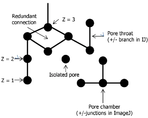
Figure 10. 2D schematic view of a pore network with several microscopic parameters represented. ... 24

Figure 11. Left-hand: 3D visualization of the mean intercept length vector for one sample. Right-hand: 3D representation of the same sample air-filled pore space aligned to the anisotropy vector. ... 27

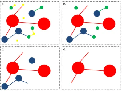
Figure 12. Schematic visible pore network with a growing visible minimal pore size (from a to d). ... 30

Figure 13. Representation of the pixels distribution of two images with different voxel size. ... 31

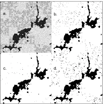
Figure 14. Image #10 at various steps: (a) simulated image 10; (b) Otsu segmentation; (c) PBA segmentation and (d) IK/GM segmentation. There was no application of a pre-segmentation filter. ... 37

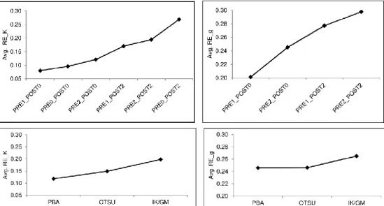
Figure 15. Averaged misclassification error (ME), region non-uniformity (NU) and porosity relative error (RE_P) for all segmentation methods (Otsu, PBA, IK/GM) and for all pre-segmentation noise reductions (PRE0, PRE1, PRE2) ... 37 Figure 16. Resulting Image #10 after the OTSU and the IK/GM segmentation methods for two level of pre-segmentation noise reduction (PRE1, PRE2). Black pixels represent the pores that match the ground-truth information, the blue pixels

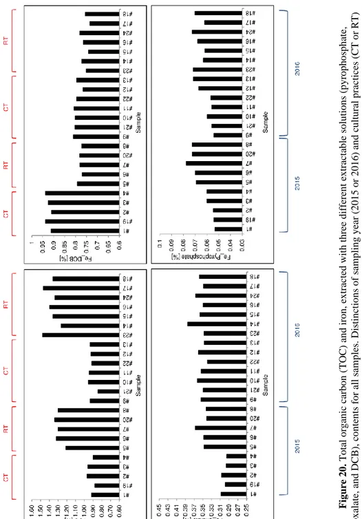
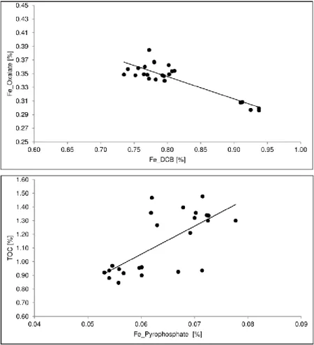
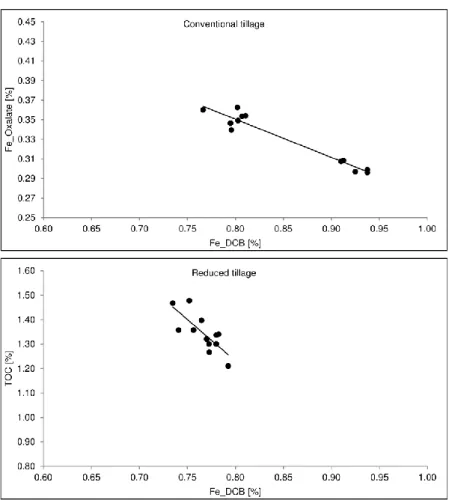
represent pixels that are allocated to soil matrix but should have been allocated to pore and the red pixels are the one allocated to pore but should not have been. ... 38 Figure 17. Left-hand: Main effect plots for the conductance relative error (RE_K). Right hand: Main effect plots for the shape factor relative error (RE_g). The upper graphs display the pre-segmentation (PRE0, PRE1, PRE2) and post-segmentation (POST0, POST2) noise reductions combinations as variables. The lower graphs display the segmentation methods as variables (PBA, Otsu, IK/GM). ... 39 Figure 18. Image #14 grayscale histograms with different pre-segmentation noise reductions. Left to right: PRE0, PRE1, and PRE2. The dotted line represents the global threshold obtained with PBA segmentation method; the plain bold line represents the upper threshold obtained with IK/GM segmentation. ... 40 Figure 19. Logarithmic laboratory measured air permeability [ka, µm²] versus logarithmic laboratory measured air-filled porosity for all soil samples at all water matric potentials. ... 44 Figure 20. Total organic carbon (TOC) and iron, extracted with three different extractable solutions (pyrophosphate, oxalate, and DCB), contents for all samples. Distinctions of sampling year (2015 or 2016) and cultural practices (CT or RT) are noted in blue and red, respectively. ... 47 Figure 22. Upper graph: Iron content extracted with oxalate (Fe_Oxalate) versus iron extracted with DCB (Fe_DCB) for all soil samples. Lower graph: Total organic carbon (TOC) versus iron extracted with pyrophosphate (Fe_Pyrophosphate) for all soil samples. ... 48 Figure 23. Total organic carbon (TOC) versus iron extracted with DCB (Fe_DCB) for both sampling year. ... 49 Figure 24. Upper graph: Iron content extracted with oxalate (Fe_Oxalate) versus iron extracted with DCB (Fe_DCB) for the samples from the conventional tillage experiment. Lower graph: Total organic carbon (TOC) versus iron extracted with DCB (Fe_DCB) for the samples from the reduced tillage experiment. ... 50 Figure 25. Grayscale histogram of the sample #1 3D image scanned at a water matric potential of -10 kPa. ... 52 Figure 26. First, second and third dimensions of the variables principal components. ... 53 Figure 27. Vertical slice in the middle of sample #1. ... 55 Figure 28. Laboratory measured volumetric water content at a water matric potential of -1500 kPa versus the microscopic average volume of the biggest pores (Avg_Bvol). ... 56 Figure 29. 3D representation of an artificial soil pore network with solid phase in brown, water phase in blue and air phase in white. The red dot on the soil water

v

retention curve indicates the water matrix potentials at which the snapshot was taken (Source: Daly et al., 2018). ... 57 Figure 30. Logarithmic saturated hydraulic conductivity (Ks) versus global connectivity (Γ) calculated from the cluster size distribution extracted from BoneJ. ... 58 Figure 31. Logarithmic saturated hydraulic conductivity (Ks) versus the fractal dimension measured on X-ray µCT images (FD). ... 59 Figure 32. Application of the group 1 and group 2 regression models. ... 60 Figure 33. Logarithmic saturated hydraulic conductivity (Ks) versus the soil degree of anisotropy measured on X-ray µCT images (DA). ... 61 Figure 34. Upper graph: logarithmic air permeability measured at a water matric potential of -70kPa (ka) versus the average pore volume of the smallest pores (Avg_Svol). Lower graph: the predicted logarithmic air permeability (ka) from the average pore volume of the smallest pores (Avg_Svol) and all pores (Avg_Vol) versus the observed logarithmic air permeability. Error bars represent the 75% regression model quantiles. ... 64 Figure 35. Pore repartition measured by pressure plates (green line), desorption-sorption vapor (blue line), on X-ray µCT images of the soil aggregate (red line), and on X-ray µCT image of the soil sample at a voxel size of 43³ µm³ (black line) and 21.5³µm³ (yellow line). ... 67 Figure 36. Pore repartition measured on X-ray µCT images (43³ µm³) of several soil samples. ... 67 Figure 37. 3D representation of the soil aggregate (left) and the soil sample #12 (right). ... 68 Figure 38. Upper row: Grayscale X-ray µCT images with the identified pore space in white. Lower row: Zoom-in of the binary X-ray µCT images. The original resolution (21.5³ µm³) is on the left-hand side and the coarsened resolution (43³ µm³) on the right-hand side. ... 70 Figure 39. Upper row: X-ray µCT grayscale image of sample #20 scanned at -30 kPa with the green volume of the difference in identified pore space between -30 kPa and -4 kPa. Lower row: One slice of the X-ray µCT grayscale image of sample #20 scanned at -4 kPa (left-hand) and at -30 kPa (right-hand). ... 73 Figure 40. Proportion of isolated porosity (IPO, %) values by samples and water matric potential (h). ... 75 Figure 41. Degree of anisotropy (DA, -) values by samples and water matric potential (h). ... 75 Figure 42. First and second dimensions of the individuals principal components for ten samples. One color per sample. ... 79

Figure 43. First and second dimensions of the variables principal components. The variables are the X-ray µCT global parameters. Refer to Table 3 for the definitions of the microscopic parameters. ... 80 Figure 44. Pore size distribution at various water matric potential for three samples. ... 82 Figure 45. Tortuosity measured on the X-ray µCT images (τ) versus Fe extracted with DCB (Fe_DCB) for all soil samples. ... 84 Figure 46. Upper-graph: The Euler number calculated on the X-ray µCT images (ε) versus the total organic carbon content (TOC) for all samples. Lower-graph: Tortuosity calculated on the X-ray µCT images (τ) versus the Fe extracted with DCB (Fe_DCB) for the samples from the CT experiment. ... 85

vii

List of tables

Table 1. Dimensionless conductance (g) calculation depending on shape factor values (G). ... 15 Table 2. Performed cultural practices between 2013 and 2016 on the sampling field. ... 20 Table 3. PartI. Calculated microscopic parameters on the X-ray µCT images and their definition. Only the parameters with a star were calculated for all soil samples at various water matric potentials. The parameters with an italic font were calculated by pore size range. ... 25 Table 4. Enumeration of the available data to evaluate the resolution effects on the calculated microscopic parameters. ... 32 Table 5. Logarithmic saturated hydraulic conductivities (Ks, cm/day) and air permeability (ka, µm²) measured of -4 kPa, -7 kPa, -10 kPa, -30 kPa and -70 kPa (minimum values [Min], maximum values [Max], mean values [Mean] and standard deviation [St dev]) ... 45 Table 6. Laboratory measured air-filled porosity at a water matric potential of -1 kPa (Lab_PO) and the fractal dimension extracted from the laboratory measured soil water retention curve (Lab_FD) for all soil samples. ... 46 Table 7. Global threshold (TH) values for all soil samples scanned at a water matric potential of -70 kPa ... 51 Table 8. Logarithmic saturated hydraulic conductivity (Ks), degree of anisotropy calculated on X-ray µCT images (DA), and corresponding characteristics for the calibration data set samples. ... 62 Table 9. Porosity indicators of the scanned sample (43³ and 21.5³ µm³) and aggregate (8.99³µm³), and from the extrapolation equations. ... 69 Table 10. Connectivity indicators of the scanned sample (43³ and 21.5³ µm³) and aggregate (8.99³ µm³). ... 71 Table 11. Observed and predicted logarithmic values of the saturated hydraulic conductivity (Ks) and air permeability measured at a water matric potential of -70 kPa (ka) for sample #12. Predictions performed from the microscopic parameters extracted from the original resolution X–ray µCT images (21.5³ µm³) and coarsened resolution (43³ µm³) X-ray µCT images. ... 72 Table 12. ANOVA results for the global parameters between water matric potentials (expressed in absolute values). Refer to Table 3 for the definitions of the microscopic parameters. ... 76

Table 13. Relative efficiency of the ANCOVA over the ANOVA performed on the global parameters (columns) with associated covariates (rows). Refer to Table 3 for the definitions of the microscopic parameters. ... 77 Table 14. K-clustering analysis from the fourth principal component analysis dimensions. The cluster numbers are identical to the sample numbers. ... 79 Table 15. Significant differences in local parameters between all water matric potentials. Refer to Table 3 for the definitions of the microscopic parameters. ... 81 Table 16. Correlations between Fe_DCB, or Fe_oxalate, and several microscopic parameters. Refer to Table 3 for the definitions of the microscopic parameters. ... 84

ix

List of abbreviations and symbols

µCT Micro-computed tomography

BF Bayes Factor

CT Conventional tillage

DVS Desorption vapor sorption

Fe_DCB Relative content of soil Fe extracted with

dithionite-citrate [MM-1]

Fe_oxalate Relative content of soil Fe extracted with oxalate

[MM-1]

Fe_pyrophosphate Relative content of soil Fe extracted with

pyrophosphate [MM-1]

G Shape factor [-]

h Water matric potential [ML-1T-2]

IK Indicator-kriging

IK/GM Indicator kriging combined to the gradient masks

threshold selection

IK/PBA Indicator kriging combined to the porosity-based

threshold selection

K(θ) Hydraulic conductivity as a function of water

content [LT-1]

ka(ε) Air permeability as a function of air-filled content

[L²]

Ks Saturated hydraulic conductivity [LT-1]

Lab_FD Fractal dimension extracted from the laboratory

measured soil water retention curve [-]

Lab_PO Laboratory measured air-filled porosity at a water

matric potential of -1 kPa [L3L-3]

ME Misclassification error [-]

MIL Mean intercept length

NU Region non-uniformity [-]

PBA Porosity-based

PCA Principal component analysis

POST0 No post-segmentation median filter

POST2 Post-segmentation median filter with a radius of two

pixels

PP Pressure plates

PRE1 Pre-segmentation median filter with a radius of one pixel

PRE2 Pre-segmentation median filter with a radius of two

pixels

r Pore radius [L]

RE_g Relative error on the conductance value [-]

RE_K Relative error on the global conductance value [-]

RRMSE Relative root mean square error [-]

RT Reduced tillage

SOM Soil organic matter

SWRC Soil water retention curve

TH Threshold

TOC Total organic carbon [MM-1]

θ Water content [L3L-3]

1

Introduction

It is no surprise the FAO proclaimed 2015 as the year of the soil: this thin continuum layer linking plants and atmosphere plays fundamentals roles in almost all environmental processes. Besides providing the land to food production or the resources for construction or industrial materials, the soil is an invisible and silent machine permanently working in providing the ground for (micro-) organisms, nutrients cycles, water filtration and storage… The numerous functions that the soil holds make it essential in regulating natural events or global climate, and place it at the heart of countless agricultural or industrial applications: the soil functions therefore need to be predictable. Predictability of the soil functions comes through the adequate simulation of the soil processes which, in particular, require a detailed characterization of the soil physical properties. The soil physical properties are traditionally approached by the texture, bulk density, retention curve, and air and water permeability. Soil field descriptions are based on averaging procedure by statistically choosing sampling points across the field, although heterogeneity is the rule at every scale (e.g., Baveye and Laba, 2015). Moreover, it is also cumbersome and delicate to characterize the soil in its unsaturated state, where convective fluxes of air and water are dependent on the degree of saturation. A complete and continuous characterization of the soil physical properties is however needed for the resolution, for example, of physical equations that predict the air and water fluxes across the soil. The use of models producing expression of the hydraulic conductivity as a function of the soil water content [K(θ)], or of the air permeability as a function of the soil air content [ka(ε)], is therefore unavoidable.

Oldest ka(ε) models were based on power-law functions with one discrete measure of ka(ε) and an empirical exponent that represented the soil pore space structure

(Buckingham, 1904; Millington and Quirk, 1961). These were modified to take into account the soil density (Deepagoda et al., 2011), the pore size distribution (Moldrup et al., 2001, Moldrup et al., 2003), or the particle size distribution (Arthur et al., 2012; Hamamoto et al., 2009). As well, it exists multiple conductivity functions that produce simple analytical expression of K(θ) from the saturated hydraulic conductivity (Ks) value and a pore size distribution model, where pores are assumed to be capillaries, such as the ones from Burdine (1953) or Mualem (1956). We can cite the model of van Genuchten et al. (1980) which is widely used. Dane et al. (2011) also proposed a model of K(θ) where the pore size distribution was extracted from discrete measures of ka(ε). It is indeed tempting to link air and water permeability measurements (Blackwell et al., 1990; Loll et al., 1999), although no perfect match between water conductivity and air permeability should be expected since water present more affinity to soil particles than air (Loll et al., 1999).

It is the usual norm to use the quoted models, but these have a major drawback: they are not physically interpretable (Hunt et al., 2013). After having considered the pore as capillaries for decades, the trend is now to objectify the fundamentals behind an observed hydrodynamic behavior. The pore space is rather seen as a collection of pore chambers connected to each other by pore throats of smaller section, or as a continuum across the soil that should not be partitioned. The direct visualization of

Introduction

3

the pore space was an incredible step forward to that purpose. For example, Vogel (1997) postulated that the discrepancy between pore size distributions extracted from soil water retention curve measurements and from serial section images was likely due to the pore space connectivity expressed by the Euler characteristic. Serial sectioning was indeed firstly used by the soil community (e.g. Cousin et al., 1996) but the samples preparation is time-consuming and requires a skilled experimenter. Considering the resolution, X-ray microcomputed tomography (X-ray µCT) is an equivalent technique with the advantage of being non-destructive and less time-consuming because no sample preparation is needed (such as the resin impregnation with serial sectioning). X-ray µCT technique is now widely used in soil science. Landis and Keane (2010) propose a full description of the technology, and Taina et al. (2007) and Wildenschild and Sheppard (2013) discuss the use of X-ray µCT to study the vadose zone. In soil science, the technique has been used at both the core (e.g., Jassogne et al., 2007; Elliot et al., 2010; Luo et al., 2010a.; Larsbo et al., 2014; Katuwal et al., 2015b), and aggregate scale (e.g., Peth et al., 2008; Papadopoulos et al., 2009; Kravchenko et al., 2011) for describing the microscopic pore space morphological and topological structure and studying the impact of land use and agricultural management on soil structure (e.g., Jassogne et al., 2007; Peth et al., 2008; Papadopoulos et al., 2009; Luo et al., 2010a.; Kravchenko et al., 2011) as well as for analyzing the relationships between soil pore space structure and soil physical properties (e.g., Elliot et al., 2010; Larsbo et al., 2014; Katuwal et al., 2015b). As already stated, the heterogeneity is the rule at every scale, and each soil sample presents a unique pore space size distribution and morphological or topological connectivity. Studying the link between the microscopic pore space structure of a sample and its specific fluid transport properties is therefore a step forward in our understanding of how the microscopic soil structure affects the soil functions. On one hand, experimentally visualized infiltration studies shed light on the effective conducting pore space which represents only a small portion of the total pore space (Luo et al., 2008; Koestel and Larsbo, 2014; Sammartino et al., 2015). The procedures developed in these studies are promising, but restricted, as stated in their objectives, to the analysis of large macropores because of the trade-off between resolution and acquisition time. On the other hand, numerical simulations performed on pore space grid are used to predict conductivity. Many studies focus on idealized porous structures (e.g., Vogel et al., 2005; Schaap et al., 2007) and a few deals with actual soil (Elliot et al., 2010; Dal Ferro et al., 2015, Tracy et al., 2015). The latter show encouraging results, but restricted to a defined resolution and/or sample size (Baveye et al., 2017). Indeed, the direct approach of linking one microscopic pore space structure to one soil function is limited by the difficulty in analyzing the structure in a representative way, so that the soil would be adequately characterized (Vogel et al., 2010). The description of soil pore space structure via global characteristics could encompass that challenge and comparisons of one soil sample microscopic structure to its own sample-scale properties have indeed gained attention.

Several studies reported that the global µCT extracted macroporosity explained the sample-scale saturated hydraulic conductivity (Luo et al., 2010b; Paradelo et al., 2016; Mossadeghi-Björklund et al., 2016) or air permeability (Naveed et al., 2012; Katuwal et al., 2015b, Paradelo et al., 2016). Other microscopic measurements calculated on the X-ray µCT images were found to influence the fluid transport, such as the number of independent macropore or macropore hydraulic radius (Luo et al., 2010b), the number of pores (Lamandé et al., 2013, Anderson et al., 2014), and the fractal dimension (Anderson et al., 2014). Naveed et al. (2016) also suggested that biopore-dominated and matrix-dominated flow soil cores should be distinguished before analyzing relationships between microscopic and macroscopic soil properties. These observed relationships between flow parameters and µCT global characteristics are intuitive, but depend on image resolution, water matric potential and soil type. Moreover, the µCT porosity, number of pores, average pore radius, surface area and pore network connectivity and tortuosity all depend on the minimal visible pore size, in other words, on the resolution of the binary X-ray µCT images used to obtain the pore network (Houston et al., 2013b; Peng et al., 2014; Shah et al., 2016). The quoted studies worked with voxel size in average a thousand times larger in volumes than the one we work with, knowing useful information about conducting pores is lost with increased voxel size. For example, Sandin et al. (2017) worked at a smaller voxel size (120³ µm³) and observed significant correlations between Ks and a global measure of the pore network connectivity (from the percolation theory) which had, to our knowledge, never been observed. Pore network connectivity and tortuosity are important indicators of flow capacities (Perret et al., 1999; Vogel, 2000), but there is still a lack of information on the links between global pore network connectivity indicators and flow parameters. The first objective of our dissertation is therefore to unravel the relationships between macroscopic sample-scale soil properties and microscopic soil structure, working with a smaller voxel size (43³µm³) than other studies. Unprecedented, Bayesian statistics are used to explore the relationships between micro- and macroscopic soil data so the uncertainty inherent to the collected and processed µCT data is taken into account. The identification of the key global indicators that induce soil hydrodynamic functions would be of major interest for the generation of phenomenological pore network models.

An adjacent question although arises: would the observed relationships remain if we had worked with an even higher X-ray µCT resolution? Baveye et al. (2017) recently reviewed the studies that investigated ways to take into account the sub-resolution porosity, such as the use of gray scale images to perform Lattice-Boltzmann water and solutes fluxes simulations, or to consider that the solid phase in binary images is partially permeable. They however pointed out that the X-ray µCT images quality and processing prevent from obtaining meaningful grayscale values, and that we are far to evaluate practically the “penetrability of the voxels”. When reliable estimation of any voxels permeability would be obtained, we would still need to hypothesize about the connectivity of the sub-resolution porosity to the visible pores. To provide reflection areas, and for one soil sample, we extrapolate

Introduction

5

the X-ray µCT parameters to a lower voxel size on one hand, and we analyze the same X-ray µCT image at its original voxel size (21.5³µm³) on the other hand. In the continuity, we also scan a soil aggregate from the same soil sample at a voxel size of 8.99³ µm³ and measure its water adsorption-desorption curve to extract a physical pore size distribution. The second objective of this dissertation is therefore to evaluate the evolution of the X-ray µCT extracted parameters with image resolution.

Vogel (1997) or Parvin et al. (2017) postulated that the pore network connectivity influences the soil retention of water. Capillary theory in soil science, although being used for decades, might therefore not be representative of the occurring hydrodynamic processes. Working on the same soil samples for the microscopic pore space and macroscopic hydrodynamic properties characterization, we confirmed these hypothesis and we also reported that the pore network connectivity influences the flow of water and air. The next objective of this dissertation is therefore to explain, from a microscopic structural point of view, the inadequacy of the capillary law applied to soil. To that purpose, we visualize, quantify, and compare the air-filled pore space of twenty soil samples at five water matric potentials.

The stated objectives of this dissertation assume that the pore space description generated from the image processing accurately represents the physical reality of the sample microstructure, but the choice of X-ray µCT image processing methodology has a visible impact on the resulting structure. Figure 1 shows an example of the processing steps from sample acquisition to a binary image. Each step involves choosing the appropriate method and parameters, which are numerous and can have a profound effect on the resulting structure. These choices ultimately depend on the experience of the operator, and between soil science research papers, the applied methodology and used software differ profoundly. What is important here is, however, not only the diversity of these choices, but also the fact that they are often inadequately described or justified. Segmentation is the essential step when pixels are assigned to either the solid or porous phase. There are numerous segmentation methods; a review of those used in soil science can be found in Tuller et al. (2013). We here differentiate global and local thresholding methods. The aim of a thresholding method is to select a grayscale value, manually or automatically, that separates the image gray levels into two groups: greater than or equal to the threshold (TH); and less than TH. In soil science, these two groups are often defined as the solid phase (soil matrix) and the void phase (pore space). With global thresholding, a constant TH is chosen for the entire image, whereas with local thresholding the value is computed for every pixel, based on the local neighborhood (Tuller et al., 2013). Segmentation precision depends on the initial quality of the grayscale images. Enhancing the projections before reconstruction and the reconstructed images before segmentation is the typical approach, and an efficient method for improving image quality is to apply noise reduction filters (Kaestner et al., 2008; Wildenschild and Sheppard, 2013). Pre-segmentation processing are more

efficient at handling image degradation than post-segmentation ones: a general rule (for more than just image analysis) is that the more upstream a problem is corrected, the easier is it to process the data downstream.

Figure 1. X-ray µCT image processing steps from acquisition to binary image. Some sources

Introduction

7

Some authors have shown (Peth et al., 2008; Tarquis et al., 2009; Lamandé et al., 2013; Beckers et al., 2014b; Peng et al., 2014) that, in most practical cases, the choice of segmentation method plays a crucial role in the resulting pore structure, but no standards have yet been proposed. Several studies sought to classify thresholding techniques based on information available from the resulting binary images (Baveye et al. 2010; Houston et al., 2013b; Iassonov et al., 2009; Schlüter al., 2014). So far as we know, only Wang et al. (2011) have used synthetic soil aggregate images, from which ground-truth information was available, to compare thresholding methods. Even these studies were based on image-by-image analyses and did not provide a tool with which to properly evaluate the processing methodologies. Within this context, a transversal objective of this dissertation is to provide a statistical analysis of the segmentation processing effects on the resulting data. By evaluating Otsu’s global method (Otsu, 1979), the local adaptive-window indicator kriging (IK) method (Houston et al., 2013a) and the porosity-based (PBA) global method (Beckers et al., 2014b) on 2D simulated soil images from which ground-truth information is available, we are able to objectively support existing reviews and be confident with the used image processing methodology.

2

Materials & Methods: the methodological

2.1. Introduction

We first present a simple example which points out the difficulties in image processing decisions when no ground-truth information is available. For example, a beam hardening correction1 of 25%, which is a common procedure in X-ray µCT image processing, implies a smaller averaged pore surface area which came from a higher amount of small pores, as a consequence of the extra-noise generated by the beam hardening correction (Fig. 2). However, the gray values histogram shows a slight right-hand shift (pores in black, not shown) in histogram peaks with the 25% beam hardening correction, and this is consistent with the observations of an increasing porosity and a higher visual contrast. This could make the segmentation step more straightforward and could be used in combination to a noise reduction filter to remove the additional small noise. The correction, however, modifies the visible porosity, and therefore the structure, in an unknown way as also demonstrated by Beckers et al. (2014b).

Figure 2. Slice of a binary 3D images of the soil samples. Left-hand: a 25% beam hardening

correction was applied during reconstruction. Right-hand: no beam hardening correction was applied.

We also briefly investigated the effects of noise reduction filter on the final resulting binary images. As expected, the number of small pores decreased with the level of pre-segmentation noise reduction, as the visual contrast increased. A higher level of pre-segmentation lead to more uniform phases (Fig. 3) which induces less

1

The beam hardening artefact is due to the polychromatic nature of the X-ray beam implying that the Beer’s Law no longer holds. The images present a radial grayscale intensity variation from the edges to the center.

Materials & Methods: the methodological experiment

11

noisy binary image. Higher the median filtering is, the more information is however lost.

Answering the methodological objective was therefore a perquisite to any real soil image analysis, and we firstly present the developed procedure to that purpose and its ensuing research question which is “what segmentation method and what noise filtering level should we apply?” The methodological experiment was performed on simulated images so ground-truth information would be available for reliable evaluation of the image processing effects on the final binary image features quantification.

Figure 3. Portion of a slice from a soil sample 3D grayscale image. Left-hand: no

pre-segmentation filter was applied. Right-hand: a pre-pre-segmentation median filter with a radius of two pixels was applied.

2.2. Simulated images

Our Paper I presents the extensive procedure of the images construction. The general frame was based on the methodology from Wang et al. (2011), which consists in superimposing a realistic binary pore image to an image representing partial volume effects2 and then adding Gaussian noise (Fig. 4). We have created 15 simulated images from the combination of 15 selected real soil binary images (from Beckers et al., 2014b) to 15 different generated partial volume effect images. The tested thresholding methods should identify the pore region from the original real soil image.

2

Due to a pixel size higher than the smallest pore, the partial volume effect implies that voxels can contain more than one phase which causes the difficulty of the segmentation step.

Figure 4. Detailed illustration of the simulated images construction.

The partial volume effect images were generated through the overlaying of decreasing resolution images as proposed by Wang et al. (2011). We did not use real soil images of multiples resolutions as Wang et al. (2011) did, we instead produced fractal images of decreasing resolution with a fractal generator based on the pore-solid fractal approach (Perrier et al., 1999). Many studies reported that the fractal concept provides a good description of the soil microstructure complexity (e.g. Kravchenko et al., 2011). Those images were then combined to form one partial volume effect image; Fig. 5 displays two examples of final simulated images.

Materials & Methods: the methodological experiment

13

2.3.

Tested

image

processing

and

image

features

characterization

The complexity of segmentation is tied to the noise, artefacts and partial volume effects found in the grayscale images. Other sources of image degradation include ring artefacts, streak artefacts, high-frequency noise, scattered photons and distortions (Baruchel et al., 2000). We therefore firstly tested the effects of a pre-segmentation median filter on the pre-segmentation quality. Median filters assign the median value of the neighboring pixels to the center pixel. These filters are less sensitive to extreme values and no grayscale value is created near the object boundary implying that the object edges are better preserved (Tuller et al., 2013). The use of a median filter before segmentation seems to be a common step within the field of soil X-ray CT images processing. Three levels were tested: no filter, filter with a radius of one pixel, filter with a radius of two pixels. After enhancing the image quality, choosing the right segmentation method is crucial. We tested three segmentation methods from the literature and adapted one. After all, a post-segmentation median filter was also tested on the simulated images (no filter or filter with a radius of two pixels). A post-processing clean-up was applied by removing the pore strictly smaller than 5 pixels in area, and the pore quantification was performed with the “Analyze Particles” tool available in the public domain image processing ImageJ (Schneider et al., 2012).

2.3.1. Global segmentation methods

The global thresholding method from Otsu (Otsu, 1979) was tested since it provides acceptable results according to Iassonov et al. (2009). Despite its potential non-reliability and the existence of more recent and more efficient methods, it is still a widely used method in the case of soil images, probably for its fast and easy-to-use implementation. This method automatically chooses a threshold based on the minimization of the intra-class variance between two intensity classes of pixels. It was performed with Matlab R2015a (MathWorks, UK).

As we have ground-truth information available, threshold that should be applied can be estimated. Through an iterative loop, the threshold that minimizes the difference between calculated porosity and ground truth porosity is selected and the value will serve as a benchmark. This procedure is based on the method from Beckers et al. (2014b). The Matlab R2015a (MathWorks, UK) code was provided by the authors.

2.3.2. Local segmentation method

The indicator kriging method (Oh and Lindquist, 1999) has provided good results in various studies (Peth et al., 2008; Iassonov et al., 2009; Wang et al., 2011; Houston et al., 2013b). Its variation “window-adaptive indicator kriging method” (Houston et al., 2013a) is however chosen because Houston et al. (2013a) concluded that the adaptive method requires less computational resources than the fixed one while providing very similar results. The indicator kriging concept relies on the selection of a threshold interval, TH1-TH2. All grayscale values below TH1 are set

to 0 and all values above TH2 are set to 1. The values between TH1 and TH2 are assigned to a specific color, namely a phase, depending on their grayscale value and their classified neighboring pixels. The adaptive-window indicator kriging method adapts this neighboring area on the information locally available to cut the computational cost when possible. The method was applied with the author’s software “AWIK”. The choice of TH1 and TH2 was based on the edge detection using gradient masks method (Schlüter et al., 2010), option available within the AWIK software. From now on, we will refer to it as IK/GM.

The PBA method has shown to be satisfactory albeit revealing a lower performance than IK/GM (Beckers et al., 2014b). The weakness in IK/GM is the choice of the interval TH1-TH2. Schlüter et al. (2010) have proposed an improved automatic TH interval selection method, although it remains sensitive to noise. Therefore we wish to combine the physical robustness of the PBA method to the assumed precision of the IK method. The aim is to select a TH interval based on the global PBA threshold and then compute the IK method. This method was tested on the simulated images. We remind that the PBA method was used as a benchmark since we knew the exact porosity of the ground-truth image to be processed. From now on, we will refer to it as IK/PBA.

2.4. Results analysis

2.4.1. Performance indicators

We used the ground-truth information available to compute the misclassification error (ME), whose value is included between 0 and 1. It gives the proportion of pixel wrongly assigned to a phase. The value 0 reflects a perfect segmentation and the value 1 the opposite (Sezgin and Sankur, 2004):

0 0 0 0

1

S

P

S

S

P

P

ME













Where P0 is the number of pore pixel in the ground-truth image; PT is the number

of pore pixel in the tested image; S0 is the number of solid pixel in the ground-truth

image; ST is the number of solid pixel in the tested image. We have chosen this

simple indicator for its obvious interpretation and for the possibility of comparison with other studies (Wang et al., 2011; Schlüter et al., 2014). Similarly, we used the relative error on the calculated porosity as a performance indicator (RE_P). The calculated porosity is the ratio of black pixels (pores) over the total number of pixels.

Region non-uniformity (NU) is usually calculated to evaluate the segmentation quality without using ground-truth information (Wang et al., 2011). High intra-region uniformity is related to a suitable segmentation method because there is a similarity of property in the region element; the variance of that property is then adequate in expressing the uniformity (Zhang, 1996):

Materials & Methods: the methodological experiment

15

𝑁𝑈 =

𝑇.𝜎2 [Eq.2]

Where P is the number of pore pixel; T is the total number of pixel; σp²is the gray

values variance of the pore pixels in the original grayscale simulated image; σ² is the total gray values variance in the original grayscale simulated image. NU is a natural choice given the uniformity that the pore space should possess, although shows lower performance compared to ground-truth information based indicator (Zhang, 1996).

For each pore, we computed its shape factor as defined by Mason and Morrow (1990) (Eq. 3) where A is the surface area (pixel²) and P is the perimeter (pixel):

𝐺 =

Depending on the G value, we calculated the specific dimensionless conductance of each pore (Patzek and Silin, 2001, Table 1). The dimensionless conductance

g

~

multiplied by the squared cross-section surface area (A²) and divided by the fluid viscosity (µ), gives the conductance g (L5TM-1):

𝑔 =

The volumetric flow rate through one pore is obtained by multiplying the conductance (g) by the fluid displacement driving force. In analogy with an electric circuit where resistances are summed in series, conductances are summed in parallel. We therefore multiplied each pore dimensionless conductance (𝑔̃) by their squared surface area (A²) in order to sum all the conductances (g) for each image which resulted in a global conductance. The relative error of the global conductance to the ground truth image was calculated for each image (RE_K). In addition, we calculated the dimensionless conductance (𝑔̃) relative error of each pore (RE_g). RE_K and RE_g indicators were studied in absolute values.

Table 1. Dimensionless conductance (g) calculation depending on shape factor values (G). G value G > 1/16 (31/2)/36 < G <1/16 G < (31/2)/36

Associated shape Circle Square Triangle

2.4.2. The methodological research question

To assess whether the quality of a segmentation method is altered by noise reduction, three-way ANOVA were implemented to test for significant differences in ME, NU, RE_P and RE_K for the various levels of noise reductions and the three different segmentation methods. Randomized complete block design was applied, the simulated images being the random blocks. In case of significant fixed interaction, two-way ANOVA were conducted for each segmentation method to test for significant impact of noise reduction on segmentation results. Tukey’s post-hoc test was performed in case of significant effect (p<0.05).

Then to determine which combination of segmentation method and noise reduction performs the most accurately and whether IK/PBA brings improvement, four two-way ANOVA were implemented to test for significant difference in ME, NU, RE_P, RE_K between the combinations of segmentation method and noise reduction (10 levels). In case of significance (p<0.05), a post-hoc Dunnett test was conducted with IK/PBA as the control.

In each case, similar analyses of RE_g were conducted. However, since each pore has its own shape factor, all the 229 pores (for all 15 images combined) were each considered as a random block.

3

Materials & Methods: the field

3.1. Introduction

The field experiment consisted in the measurements of sample-scale hydrodynamic properties and microscopic X-ray µCT extracted parameters on undisturbed soil samples of 35 cm³. The length ratio between sample size (3 cm in diameter) and scanner voxel size (21.5³ µm³) was around 1400, or 700 when the µCT images were resampled to a voxel size of 43³ µm³. This is a typical ratio value which allows the identification of most of X-ray µCT image characteristics (Vogel et al., 2010). The image characteristics were the soil pore space morphological and topological features, expressed in terms of “microscopic parameters”. All of the visible soil porosity (the smallest visible pores were about 0.0004 mm³) was characterized and analyzed without distinction of origins (structural or biological) since hydrodynamic properties measurements were performed on the samples as a whole. The three research questions previously introduced are:

- Research question #1: Which microscopic parameters explain the best the soil hydrodynamic properties measured at the sample scale?

- Research question #2: How do the microscopic parameters evolve with resolution?

- Research question #3: How does the air-filled porosity vary with water matric potential?

Eventually, we also address a fourth research question regarding the likely origins of soil structure:

- Research question #4: How is the soil structure explained by organic carbon and iron content? At the origin of structure.

3.2. Soil sampling

The studied soil samples were taken from an agricultural field in Gembloux (Belgium) classified as a Cutanic Luvisol (WRB soil system, 2006) with the following averaged particle distribution: 14.3 % of clay, 78.3% of silt and 7.4% of sand. Sampling was performed within the summer 2015 (10 samples) and summer 2016 (14 samples) within four plots of a tillage-residue experiment (Fig. 6).

The tillage-residue experiment was conducted by Hiel et al. (2018) and the cultural practices between summer 2013 and summer 2016 are displayed in Table 2. Each sampling year, half of the samples were taken from the “conventional tillage” experiment, the other half from the “reduced-tillage” experiment. The objective was to observe a maximum variability of pore network structure between the samples and not to compare the experiment effects on the pore network. We therefore randomly named the samples according to a logical suite, going from #1 to #24.

After removing the vegetation, we manually drove the ertalon (plastic) cylinders (3 cm in diameter and 5 cm in height) into the soil until the top of the cylinder was at the surface level (Fig. 7) and we also manually excavated the cylinders to minimize the structure disturbance.

Materials & Methods: the field experiment

19

Figure 6. Aerial photography of the sampling field (50°56’N, 4°71’E).

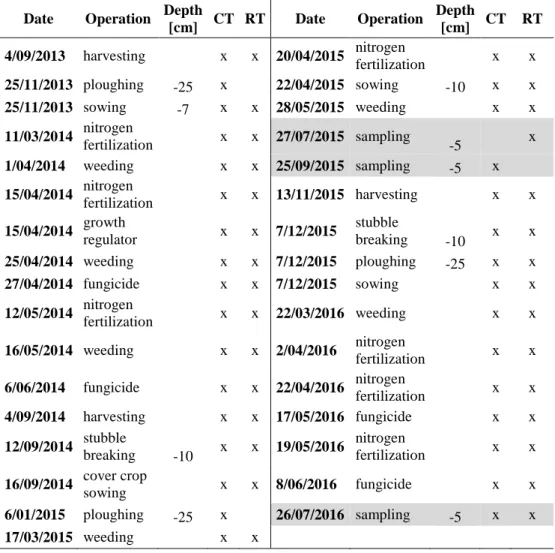
Table 2. Performed cultural practices between 2013 and 2016 on the sampling field.

Date Operation Depth

[cm] CT RT Date Operation Depth [cm] CT RT 4/09/2013 harvesting x x 20/04/2015 nitrogen fertilization x x 25/11/2013 ploughing _-25 x 22/04/2015 sowing _-10 x x 25/11/2013 sowing -7 x x 28/05/2015 weeding x x 11/03/2014 nitrogen fertilization x x 27/07/2015 sampling -5 x 1/04/2014 weeding x x 25/09/2015 sampling -5 x 15/04/2014 nitrogen fertilization x x 13/11/2015 harvesting x x 15/04/2014 growth regulator x x 7/12/2015 stubble breaking -10 x x 25/04/2014 weeding x x 7/12/2015 ploughing -25 x x 27/04/2014 fungicide x x 7/12/2015 sowing x x 12/05/2014 nitrogen fertilization x x 22/03/2016 weeding x x

16/05/2014 weeding x x 2/04/2016 nitrogen _{fertilization} x x

6/06/2014 fungicide x x 22/04/2016 nitrogen _{fertilization} x x

4/09/2014 harvesting x x 17/05/2016 fungicide x x 12/09/2014 stubble breaking -10 x x 19/05/2016 nitrogen fertilization x x 16/09/2014 cover crop sowing x x 8/06/2016 fungicide x x 6/01/2015 ploughing -25 x 26/07/2016 sampling -5 x x 17/03/2015 weeding x x

3.3. Macroscopic measurements

Figure 8 presents the general frame applied to all the soil samples except for four of these which were only scanned at a water matric potential (h) of -70 kPa. The saturation was performed with distilled water and the characteristic soil water retention curves (SRWC) were measured using pressure plates (Richards, 1948 and DIN ISO 11274, 2012). After being weighed at the specified h, the air permeability of the samples was measured by applying an air flow across the sample and measuring the resulting inner-pressure with an Eijkelkamp air permeameter 08.65 (Eijkelkamp Agrisearch Equipment, Giesbeek, The Netherlands). As recommended by the constructor, each measure was repeated five times and kept as short as possible. Corey’s law was then applied to calculate the air permeability [ka, L²]

Materials & Methods: the field experiment

21

(Corey, 1986 in Olson, 2001). The samples were also scanned at various steps of the SWRC; the X-ray microcomputed tomography procedure is developed in the next section. After reaching -1500 kPa, the soil samples were saturated once again and the saturated hydraulic conductivity (Ks [LT-1]) was measured using a constant head device (Rowell, 1994) and applying Darcy’s law. Finally, the soil samples were oven-dried at 105° for five days in order to obtain their dry weight. Porosity [L³L-3] was calculated as the ratio between the volume of water within the saturated soil sample and its total volume (McKenzie et al., 2002). From McKenzie et al. (2002), the bulk density (BD) [ML-3] was deduced from the porosity value assuming a particle density of 2.65 g/cm³. Soil organic matter content was approached by the measure of the soil organic C content through the Walkley-Black (1934) method, and the mineral constituents of the soil phase were approached by measuring the Fe content because it was shown Fe was one of the most important substrate for the formation of organo-mineral associations (Eusterhues et al., 2005). The different forms of free Fe were extracted with 1) pyrophosphate of Na to provide the quantity of complexed Fe (Bascomb, 1984); 2) Oxalate NH4 to provide the quantity of complex and amorphous Fe (Blackmore et al., 1981); and 3) dithionite-citrate system buffered with bicarbonate (Mehra and Jackson, 1960) to provide the quantity of any free forms of Fe: complex, amorphous and crystalline Fe.

3.3.1. Fractal dimension from the pore size distribution

The SWRC is usually used to extract the pore size distribution of the studied soil (Nimmo, 2004) by using the capillary theory which is the physical law linking a pore radius to a liquid potential:

𝑟 =

Where r is the pore radius (L), h is the water matric potential (L), σ is the liquid surface tension (MT²), α is the contact angle between the liquid and the soil, ρ is the liquid density (M L-3) and g is the gravitational acceleration (L T-2). That equation can be simplified when the liquid is water:

𝑟 =

Where r is the pore radius (µm), and h is the water matric potential (m).

We then calculated the fractal dimension (Lab_FD) for each pore size distributions to characterize each sample SWRC with one value. The fractal dimension is a single value that is used to characterize the fractal geometry of objects. Fractal geometry states that an object has comparable features at different scales. The fractal dimension (FD) is power-law dependent (Mandelbrot, 1983) and Fig. 9 illustrates the following equation:

𝐹𝐷 =

Where N is the constant number of transformed element at each iterations (from Eq. 7, N=2 in Fig. 9); r is the ratio between the dimension of the parent-element and the dimension of the transformed element (from Eq. 7, r=1/3 in Fig. 9). Figure 9 is a 1D fractal object (a line) and the FD should be included between 0 and 1 (FD = 0.631 in Fig. 9).