Supporting Information
Reduction of Nanoparticle Load in Cells by
Mitosis but not Exocytosis
Joël Bourquin
1, Dedy Septiadi
1, Dimitri Vanhecke
1, Sandor Balog
1, Lukas Steinmetz
1, Miguel
Spuch-Calvar
1, Patricia Taladriz-Blanco
1, Alke Petri-Fink
1,2, Barbara Rothen-Rutishauser
11
Adolphe Merkle Institute, University of Fribourg, Chemin des Verdiers 4, 1700 Fribourg,
Switzerland
2
Department of Chemistry, University of Fribourg, Chemin du Musée 9, 1700 Fribourg,
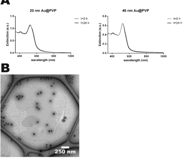
Figure S1 NP stability in cCCM. A) The 20 nm Au@PVP (left) and the 46 nm Au@PVP
NPs (right) were incubated for 24 hours in cCCM at 37 °C. Immediately after the incubation
started (red) and 24 hours later (black) their UV-Vis extinction spectra were collected. No red
shift is observed for either of the Au NPs indicating that the aggregation in cCCM is
negligible and the PVP surface coating is sufficient to stabilize the NPs. B) SiO
2NPs were
incubated in cRPMI (250 µg mL
-1) for 24 hours and further visualized using CryoTEM.
Single particles were clearly visible and little to no aggregation was observed.
Scale bar= 250 nm
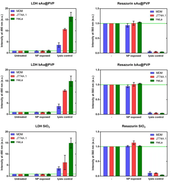
Figure S2 Cytotoxicity assays show no reduction of cell viability at 20 μg mL
-1. Neither of
the 3 different NPs (SiO
2, 20 nm Au@PVP and 46 nm Au@PVP) used showed significant
alterations in cell membrane permeability (LDH, upper panel) nor cell metabolism
(Resazurin, lower panel) for any cell type used after 24 hours of exposure and 48 hours of
post-exposure. The NP treated cells were compared to the untreated negative control and the
0.2 % Triton X-100 treated positive control.
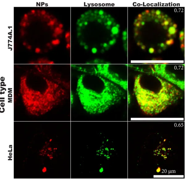
Figure S3 NP-Lysosome co-localization. Live cell imaging of the different cells previously
incubated for 24 hours with the SiO
2NPs (red) and 15 min with cCCM supplemented with a
lysosomal stain (green), co-localization appears in yellow. Co-localization coefficient is
annotated in the top right corner. Scale bar = 20 µm.
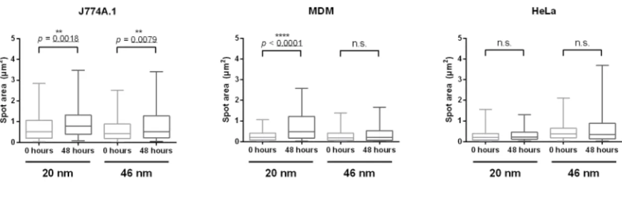
Figure S4 Average spot size increases in DF microscopy with increasing post-exposure
time. The DF micrographs were binarized using a threshold (same threshold for same
conditions) and further analyzed for their spot sizes using particle tracker from FIJI. The box
plots show medians (line in the box) and 5-95 percentiles (whiskers) of the analysis
performed for J774A.1 (A), MDM (B) and HeLa (C). Significant increases of sizes were
observed for both particle types in J774A.1 and for the 20 nm Au@PVP particles in the case
of MDMs. No significant increase was detected for any NPs in HeLa cells. Significance was
calculated using student’s t-test.
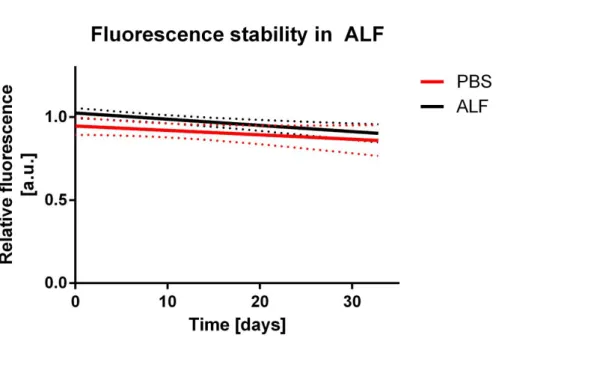
Figure S5 Stability of fluorescent particles over time in the lysosomal environment. 0.5
mg mL
-1of the fluorescently labelled SiO
2
NPs were incubated in either artificial lysosomal
fluid (ALF) or PBS. The relative fluorescence was measured after 1, 2, 3 and 30 days using a
plate reader. No significant differences in the fluorescence over time can be seen when
comparing ALF and the PBS control. Within the first 48 hours in ALF the fluorescence
remained at 97 % of the initial fluorescent signal and at 90 % after 30 days. Dotted lines: 99
% confidence band.
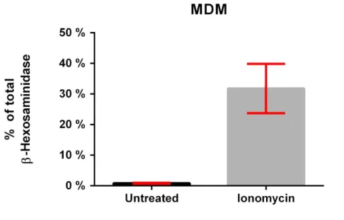
Figure S6 Release of β-Hexosaminidase by MDMs upon stimulation with ionomycin.
MDMs were exposed to 20 μM ionomycin for 6 hours. After the exposure the supernatant
was collected and the total amount of released enzyme was quantified based on its enzymatic
activity and compared to the lysed cells. Upon stimulation, approximately 30 % of the total
amount of the enzyme was released in the supernatant in contrast to the untreated control cells
that released < 1 % of the enzyme into the supernatant.
Figure S7 Flow cytometry shows little reduction of the MFI in proliferation inhibited
cells. In contrast to normal growth conditions (Figure 4A) the MFI remains on a high level in
proliferation inhibited J774A.1 (red) and HeLa (green) cells. The small amount of reduction
in the MFI can be explained by cells which were still proliferating or the release of NPs in
microvesicles induced by the stress conditions during starvation. Data is shown as the mean ±
standard deviation of 3 individual experiments. Lower panel shows J774A.1 cells grown for
24, 48 and 72 hours in the reduced serum conditions.
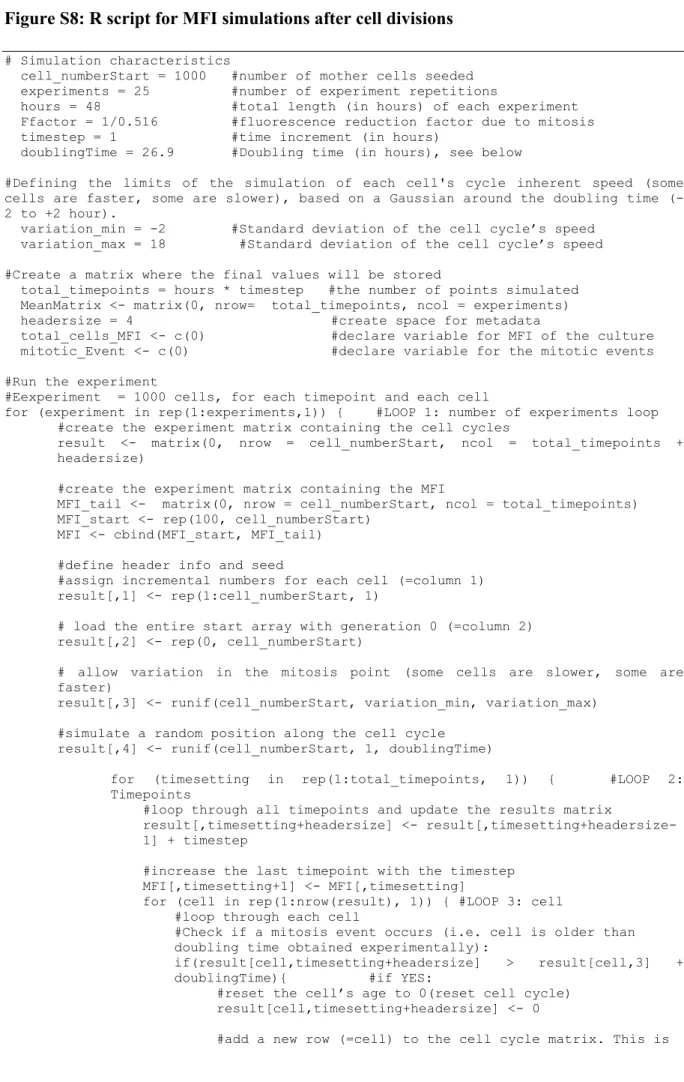
Figure S8: R script for MFI simulations after cell divisions
# Simulation characteristicscell_numberStart = 1000 #number of mother cells seeded experiments = 25 #number of experiment repetitions
hours = 48 #total length (in hours) of each experiment Ffactor = 1/0.516 #fluorescence reduction factor due to mitosis timestep = 1 #time increment (in hours)
doublingTime = 26.9 #Doubling time (in hours), see below
#Defining the limits of the simulation of each cell's cycle inherent speed (some cells are faster, some are slower), based on a Gaussian around the doubling time (-2 to +(-2 hour).
variation_min = -2 #Standard deviation of the cell cycle’s speed variation_max = 18 #Standard deviation of the cell cycle’s speed
#Create a matrix where the final values will be stored
total_timepoints = hours * timestep #the number of points simulated MeanMatrix <- matrix(0, nrow= total_timepoints, ncol = experiments)
headersize = 4 #create space for metadata
total_cells_MFI <- c(0) #declare variable for MFI of the culture
mitotic_Event <- c(0) #declare variable for the mitotic events
#Run the experiment
#Eexperiment = 1000 cells, for each timepoint and each cell
for (experiment in rep(1:experiments,1)) { #LOOP 1: number of experiments loop
#create the experiment matrix containing the cell cycles
result <- matrix(0, nrow = cell_numberStart, ncol = total_timepoints + headersize)
#create the experiment matrix containing the MFI
MFI_tail <- matrix(0, nrow = cell_numberStart, ncol = total_timepoints) MFI_start <- rep(100, cell_numberStart)
MFI <- cbind(MFI_start, MFI_tail) #define header info and seed
#assign incremental numbers for each cell (=column 1) result[,1] <- rep(1:cell_numberStart, 1)
# load the entire start array with generation 0 (=column 2)
result[,2] <- rep(0, cell_numberStart) # allow variation in the mitosis point (some cells are slower, some are
faster)
result[,3] <- runif(cell_numberStart, variation_min, variation_max) #simulate a random position along the cell cycle
result[,4] <- runif(cell_numberStart, 1, doublingTime)
for (timesetting in rep(1:total_timepoints, 1)) { #LOOP 2: Timepoints
#loop through all timepoints and update the results matrix
result[,timesetting+headersize] <- 1] + timestep
#increase the last timepoint with the timestep
MFI[,timesetting+1] <- MFI[,timesetting]
for (cell in rep(1:nrow(result), 1)) { #LOOP 3: cell #loop through each cell
#Check if a mitosis event occurs (i.e. cell is older than doubling time obtained experimentally):
if(result[cell,timesetting+headersize] > result[cell,3] +
doublingTime){ #if YES:
#reset the cell’s age to 0(reset cell cycle)
result[cell,timesetting+headersize] <- 0
daughter cell 2. The mother cell becomes Daughter cell 1. row2add < c(nrow(result)+1, result[1,2] + 1, runif(1, -1, 1), rep(0, total_timepoints+1))
result <-rbind(result,row2add)
# adjust the MFI of the mother cell based on the 51.6%
factor obtained experimentally
MFI[cell,timesetting+1] <- MFI[cell,timesetting]/Ffactor
#Update and a new row to the MFI matrix with the just calculated data
row2add <- c(rep(0, timesetting),
MFI[cell,timesetting]/Ffactor, rep(0,ncol(MFI)-timesetting-1))
MFI <- rbind(MFI, row2add)
#Update the mitotic events counter with one
mitotic_Event = mitotic_Event + 1
} #Closes IF statement
} #Closes FOR loop of cells
} #Closes FOR loop of timepoints
# The MFI matrix now contains the fluorescence of each cell at each timepoint. Now, run through the MFI matrix to sum (and average) the fluorescence values at each time point to reach the MFI of the culture at each time point.
for(timepoint in rep(1:total_timepoints, 1)) { #loop through all time
points Sumvalue = 0
for (cell in rep(1:sum(MFI[,timepoint]!=0 ), 1)){ #loop through
cells
#sum the fluorescence value of each cell in sumvalue
Sumvalue = Sumvalue + MFI[cell, timepoint]
}
#create a new matrix containing the MFI at each timepoint
MeanMatrix[timepoint, experiment] = MeanMatrix[timepoint, experiment] + Sumvalue / sum(MFI[,timepoint]!=0 )
} #close the time point loop
#print/export the results for this experiment
readout <- cat ("Experiment " , experiment , " finished (", cell_numberStart , " > " ,nrow(MFI), " cells) \n")
#Update the total MFI of all cells
total_cells_MFI = total_cells_MFI + nrow(MFI) } #Closes FOR loop of experiments
#Calculate the Mean/Median/standard deviation fluorescence intensity from the arrays
sd <- apply(MeanMatrix, 1, sd) mean <- apply(MeanMatrix, 1, mean) median <-apply(MeanMatrix, 1, median)
#Output the data as a plot of the MFI over all timepoints and summarize the simulation
plot(mean)
readout <- cat("Started with ", experiments * cell_numberStart , " mother cells and ended with " , total_cells_MFI, " daughter cells after " , mitotic_Event, " mitotic events")