DEEP LEARNING STRUCTURAL AND HISTORICAL FEATURES FOR ANTI-PATTERNS DETECTION
ANTOINE BARBEZ
DÉPARTEMENT DE GÉNIE INFORMATIQUE ET GÉNIE LOGICIEL ÉCOLE POLYTECHNIQUE DE MONTRÉAL
MÉMOIRE PRÉSENTÉ EN VUE DE L’OBTENTION DU DIPLÔME DE MAÎTRISE ÈS SCIENCES APPLIQUÉES
(GÉNIE INFORMATIQUE) DÉCEMBRE 2018
c
ÉCOLE POLYTECHNIQUE DE MONTRÉAL
Ce mémoire intitulé:
DEEP LEARNING STRUCTURAL AND HISTORICAL FEATURES FOR ANTI-PATTERNS DETECTION
présenté par: BARBEZ Antoine
en vue de l’obtention du diplôme de: Maîtrise ès sciences appliquées a été dûment accepté par le jury d’examen constitué de:
Mme BOUCHENEB Hanifa, Doctorat, présidente
M. KHOMH Foutse, Ph. D., membre et directeur de recherche
M. GUÉHÉNEUC Yann-Gaël, Doctorat, membre et codirecteur de recherche M. MERLO Ettore, Ph. D., membre
DEDICATION
To my beloved parents who always supported me, and to kiki who was always there for me. . .
ACKNOWLEDGEMENTS
I would like to express my deepest gratitude to Prof. Foutse Khomh and Prof. Yann-Gaël Guéhéneuc for being my supervisor and co-supervisor respectively at Polytechnique Montréal and Concordia University.
Thank you Foutse Khomh for your guidance and for always pushing me in the right direction. Thank you Yann-Gaël Guéhéneuc for your time, your advises and your constant kindness during these two years.
I would also like to thank the examining committee for taking the time to read and review this thesis.
I would also like to express my thanks to all the members of the SWAT and Ptidej teams, it has been a pleasure working with you. Particularly, I would like to thank Rodrigo Morales, Manel Abdellatif, Cristiano Politowski, Rubén Saborido Infantes, Satnam Singh, Vaibhav Jain, Prabhdeep Singh and Loïc Fontaine for helping me building my oracle.
RÉSUMÉ
Les systèmes logiciels sont devenus une des composantes principales de tous les secteurs d’activité. Dans la course au rendement économique, les développeurs sont susceptibles d’im-plémenter des solutions non optimales aux problèmes qui leur sont posés. On nomme ainsi anti-patrons ou “design smells” ces mauvais choix de conception introduits par manque de temps et–ou d’expérience. Si ces derniers n’ont pas forcément d’impact à l’exécution, de nom-breuses études ont mis en lumière leur influence négative sur la maintenabilité des systèmes. De nombreuses approches de détection automatique des anti-patrons ont été proposées. Pour la plupart, ces approches reposent sur l’analyse statique du code, mais il a été montré que les anti-pattrons sont aussi détectables par une analyse des données historiques des systèmes. Cependant, aucune d’entre elles ne semble clairement se distinguer des autres, et chaque ap-proche identifie des ensembles d’occurrences différents, en particulier quand celles-ci reposent sur des sources d’information complémentaires (i.e., structurelles vs. historiques).
Plusieurs approches basées sur l’apprentissage automatique ont tenté d’adresser ce problème. Toutefois, ces approches semblent faire face à des limitations qui leur sont intrinsèques. D’une part, inférer des caractéristiques de haut niveau sur les systèmes à partir de données brutes nécessite des modèles d’une grande complexité. D’autre part, l’entrainement de tels modèles requière un nombre conséquent d’exemples d’apprentissage, qui sont fastidieux à produire et existent en nombre très limité.
Ce travail tire profit des méthodes d’apprentissage automatique pour répondre aux limitations évoquées précédemment. Dans un premier temps, nous proposons une méthode ensembliste permettant d’agréger plusieurs outils de détection. Nous montrons qu’une telle méthode atteint des performances nettement supérieures à celles des outils ainsi agrégés et permet de générer des instances d’apprentissage pour des modèles plus complexes à partir d’un nombre raisonnable d’exemples. Ensuite, nous proposons un modèle d’apprentissage profond pour la détection des anti-patrons. Ce modèle est basé sur l’analyse de l’évolution des métriques logicielles. Plus précisément, nous calculons les valeurs de certaines métriques pour chaque révision du système étudié, et, entrainons un réseau de neurones convolutif à y détecter les anti-patrons à partir de ces données. Nous montrons qu’en s’appuyant ainsi sur les aspects structurels et historiques des systèmes, notre modèle surpasse les approches existantes. Nos approches ont été expérimentées dans le cadre de la détection de deux anti-patrons populaires : God Class et Feature Envy, et leurs performances comparées avec celles de l’état de l’art.
ABSTRACT
Software systems are constantly modified, whether to be adapted or to be fixed. Due to the exigence of economic performances, these modifications are sometimes performed in a hurry and developers often implement sub optimal solutions that decrease the quality of the code. In this context, the term “anti-pattern” have been introduced to represent such “bad” solutions to recurring design problems.
A variety of approaches have been proposed to identify the occurrences of anti-patterns in source code. Most of them rely on structural aspects of software systems but some alternative solutions exist. It has been shown that anti-patterns are also detectable through an analysis of historical information, i.e., by analyzing how code components evolve with one another over time. However, none of these approaches can claim high performances for any anti-pattern and for any system. Furthermore different approaches identify different sets of occurrences, especially when based on orthogonal sources of information (structural vs. historical). Several machine-learning based approaches have been proposed to address this issue. However these approaches failed to surpass conventional detection techniques. On the one hand, learning high level features from raw data requires complex models such as deep neural-networks. On the other hand, training such complex models requires substantial amounts of manually-produced training data, which is hardly available and time consuming to produce for anti-patterns.
In this work, we address these issues by taking advantage of machine-learning techniques. First we propose a machine-learning based ensemble method to efficiently aggregate various anti-patterns detection tools. We show that (1) such approach clearly enhances the perfor-mances of the so aggregated tools and; (2) our method produces reliable training instances for more complex anti-pattern detection models from a reasonable number of training exam-ples. Second we propose a deep-learning based approach to detect anti-patterns by analyzing how source code metrics evolve over time. To do so, we retrieve code metrics values for each revision of the system under investigation by mining its version control system. This information is then provided as input to a convolutional neural network to perform final prediction. The results of our experiments indicate that our model significantly outperforms existing approaches.
We experiment our approaches for the detection of two widely known anti-patterns: God Class and Feature Envy and compare their performances with those of state-of-the-art.
TABLE OF CONTENTS
DEDICATION . . . iii
ACKNOWLEDGEMENTS . . . iv
RÉSUMÉ . . . v
ABSTRACT . . . vi
TABLE OF CONTENTS . . . vii
LIST OF TABLES . . . x
LIST OF FIGURES . . . xi
LIST OF ABBREVIATIONS AND NOTATIONS . . . xii
CHAPTER 1 INTRODUCTION . . . 1
1.1 Context and Motivations . . . 1
1.2 Research Objectives . . . 2
1.3 Research Contributions . . . 3
1.4 Thesis Structure . . . 4
CHAPTER 2 BACKGROUND ON SUPERVISED LEARNING . . . 5
2.1 Classification . . . 5
2.2 Models . . . 6
2.2.1 Logistic Regression . . . 6
2.2.2 Multi-layer Perceptron . . . 8
2.2.3 Convolutional Neural Network . . . 10
2.3 Optimization . . . 12
2.3.1 Loss Function . . . 12
2.3.2 Gradient Descent . . . 12
2.3.3 Hyper-parameters Calibration . . . 13
CHAPTER 3 LITERATURE REVIEW . . . 15
3.1 Definitions . . . 15
3.1.2 Feature Envy . . . 15
3.2 Detection Techniques . . . 17
3.2.1 God Class . . . 17
3.2.2 Feature Envy . . . 20
3.3 Empirical Studies on Anti-patterns . . . 23
3.3.1 Impact of Anti-patterns on Software Quality . . . 23
3.3.2 Evolution and Presence of Anti-patterns . . . 24
CHAPTER 4 STUDY BACKGROUND . . . 26
4.1 Studied Systems . . . 26
4.2 Building a Reliable Oracle . . . 27
4.3 Evaluation Metrics . . . 28
4.4 Training . . . 29
4.4.1 Custom Loss Function . . . 29
4.4.2 Optimization . . . 30
4.4.3 Regularization . . . 31
4.4.4 Ensemble Learning . . . 32
CHAPTER 5 A MACHINE-LEARNING BASED ENSEMBLE METHOD FOR ANTI-PATTERNS DETECTION . . . 33
5.1 Introduction . . . 33
5.2 SMart Aggregation of Anti-pattern Detectors . . . 35
5.2.1 Baseline . . . 35
5.2.2 Overview . . . 36
5.2.3 Input . . . 37
5.3 Evaluation of the Detection Perfomances . . . 40
5.3.1 Study Design . . . 40
5.3.2 Parameters Calibration . . . 41
5.3.3 Analysis of the Results . . . 42
5.4 Evaluation of the Ability to Label Training Instances . . . 44
5.4.1 Study Design . . . 44
5.4.2 Parameters Calibration . . . 45
5.4.3 Analysis of the Results . . . 45
5.5 Conclusion and Future Work . . . 46
CHAPTER 6 DEEP-LEARNING ANTI-PATTERNS DETECTION FROM CODE MET-RICS HISTORY . . . 48
6.1 Introduction . . . 48
6.2 CAME: Convolutional Analysis of Metrics Evolution . . . 50
6.2.1 Overview . . . 50 6.2.2 Input . . . 51 6.2.3 Architecture . . . 52 6.3 Experiments . . . 53 6.3.1 Study Design . . . 53 6.3.2 Hyper-parameters Calibration . . . 54
6.3.3 Analysis of the Results . . . 55
6.4 Conclusion and Future Work . . . 56
CHAPTER 7 THREATS TO VALIDITY . . . 58
7.1 Construct Validity . . . 58 7.2 Internal Validity . . . 58 7.3 External Validity . . . 59 CHAPTER 8 CONCLUSION . . . 60 8.1 Synthesis . . . 60 8.2 Future Work . . . 62 RÉFÉRENCES . . . 63
LIST OF TABLES
Table 4.1 Characteristics of the Studied Systems . . . 26
Table 4.2 Characteristics of the Oracle . . . 28
Table 4.3 Confusion Matrix for Anti-patterns Detection . . . 28
Table 5.1 Hyper-parameters Calibration of SMAD . . . 41
Table 5.2 Hyper-parameters Calibration of the Competitive Tools . . . 42
Table 5.3 Performances Evaluation of SMAD for God Class detection . . . 42
Table 5.4 Performances Evaluation of SMAD for Feature Envy detection . . . . 42
Table 5.5 Characteristics of the Systems used to Generate Training Instances . 45 Table 5.6 Hyper-parameters Calibration of the Subject Model . . . 45
Table 5.7 Performances of the Subject Model Trained on Injected vs Generated Smells . . . 46
Table 6.1 Hyper-parameters Calibration of CAME . . . 54
Table 6.2 Hyper-parameters Calibration of the Concurrent MLP . . . 55
LIST OF FIGURES
Figure 2.1 Graph Representation of Logistic Regression . . . 7
Figure 2.2 Graph Representation of Multi-class Logistic Regression . . . 7
Figure 2.3 Graph Representation of an Artificial Neuron . . . 8
Figure 2.4 Examples of Activation Functions . . . 8
Figure 2.5 Architecture of a MLP model . . . 9
Figure 2.6 Convolution of a 4 × 5 tensor by a 1 × 2 filter . . . 10
Figure 2.7 2 × 2 max-pooling of a 4 × 4 feature map . . . 11
Figure 2.8 Architecture of a CNN model . . . 11
Figure 2.9 Gradient Descent Algorithm . . . 13
Figure 3.1 Feature Envy example . . . 16
Figure 3.2 Move Method Refactoring solution . . . 16
Figure 3.3 Lanza and Marinescu (2007) detection rule for God Class. . . 18
Figure 3.4 Moha et al. (2010) Rule Card for God Class detection. (Hexagons are anti-patterns, gray ovals are code smells, and white ovals are properties). 18 Figure 3.5 Lanza and Marinescu (2007) detection rule for Feature Envy. . . 21
Figure 3.6 Liu et al. (2018) architecture for Feature Envy detection. . . 23
Figure 4.1 Comparison of feeding approaches: (a) gradient descent, (b) mini-batch SGD, (c) imbalanced-batch SGD. Colors represent instances belonging to same systems. . . 31
Figure 5.1 Overview of SMAD detection process . . . 37
Figure 6.1 Workflow of CAME . . . 50
LIST OF ABBREVIATIONS AND NOTATIONS
Abbreviations
ANN Artificial Neural Network
API Application Programming Interface ATFD Access To Foreign Data
AST Abstract Syntax Tree BDTEX Bayesian Detection Expert
CAME Convolutional Analysis of Metrics Evolution CNN Convolutional Neural Network
CSV Comma Separated Values
DECOR DEtection and CORrection of Design Flaws FDP Foreign Data Providers
HIST Historical Information for Smell deTection LAA Locality of Attribute Accesses
LCOM Lack of Cohesion in Methods LOC Lines Of Code
MLP Multi-layer Perceptron
NAD Number of Attributes Declared NMD Number of Methods Declared
PADL Pattern and Abstract-level Description Language relu rectified linear unit
SGD Stochastic Gradient Descent SHA Secure Hash Algorithm
SMAD SMart Aggregation of Anti-pattern Detectors tanh hyperbolic tangent
TCC Tight Class Cohesion UML Unified Modeling Language WMC Weighted Method Count
Notations K number of classes N number of instances m number of attributes c class x attribute, x ∈ R
x input vector (i.e., instance), x = [x1, x2, ..., xm]
y label for a single class, y ∈ [0, 1]
y label for a multi-class problem, y = [y1, y2, ..., yK], ∃!k | yk = 1
D training set, D = {(xi, yi)}Ni=1
w weight of a neuronal connection, w ∈ R w weights vector, w = [w0, w1, ..., wm] W weights matrix, W = [w1, w2, ..., wMl] θ set of weights, θ = {Wl}L+1l=1 f output vector, f = [f1, f2, ..., fk] = [Pθ(c1|x1), Pθ(c2|x2), ..., Pθ(cK|xK)] p(.) probability distribution P (.) probability
L number of hidden layers M hidden layer size
L(.) loss function η learning rate
λ L2 regularization hyper-parameter
Pkeep probability to keep a neuron in dropout
CHAPTER 1 INTRODUCTION
1.1 Context and Motivations
Software systems are becoming one of the key components of every industry. Thus, main-taining software quality at a high level while constantly innovating is a major issue for every company. Software quality is impacted by the patterns applied and followed by developers. Among these patterns, design patterns and anti-patterns have been shown in the literature to impact the maintenance and evolution of systems.
Design patterns (Gamma et al. (1994)) and anti-patterns (Brown et al. (1998)) have been in-troduced to encode the “good” and “bad” design practices of experienced software developers. Design patterns describe solutions to common recurring design problems and promote flexi-bility and reusaflexi-bility. Design anti-patterns present common recurring design problems, i.e., “bad” solutions that decrease some quality characteristics, and suggest “good” alternative solutions.
Anti-patterns are typically introduced in the source code of systems when developers imple-ment suboptimal solutions to their problems due for example to a lack of knowledge and–or time constraints. For instance, the God Class anti-pattern refers to the situation in which a class centralizes most of the system intelligence and implements a high number of responsi-bilities. Such classes appear when developers always assign new functionalities to the same class, thus breaking the principle of single responsibility.
There have been many empirical studies aiming to understand the effect of design anti-patterns on software systems. These works have highlighted their negative impact on software comprehension (Abbes et al. (2011)), fault-proneness (Khomh et al. (2012)) and maintain-ability (Yamashita and Moonen (2013)).
In response to these works, several strategies have been proposed to identify the occurrences of anti-patterns in software systems. Most of these works describe anti-patterns using struc-tural metrics (e.g., cyclomatic complexity or lines of code) and attempt to identify bad motifs in models of the source code by defining thresholds to apply to the value of these metrics. For example, Moha et al. (2010) proposed a domain-specific language to describe and gen-erate detection algorithms for anti-patterns using structural and lexical metrics. Alternative solutions have also been proposed to detect anti-patterns using others aspects of software sys-tems. For instance, Palomba et al. (2013, 2015a) have shown that number of anti-patterns impact how source code entities, i.e., classes and methods, evolve with one another when
changes are applied to the systems. Therefore, they proposed a set of rules designed to identify occurrences of anti-patterns from co-changes occurring between source code entities. Even though these approaches have shown acceptable detection performances, they still ex-hibit large numbers of false positives and misses, and none of them seem to truly stand out among others. Besides, a low agreement can be observed between different approaches (Fontana et al. (2012)) because each of them is based on a different definition of anti-patterns. Thus, each approach can identify occurrences that cannot be detected by others, especially when they rely on orthogonal sources of information (Palomba et al. (2013)).
Recently, machine-learning models have been shown efficient in a variety of domains. Specifi-cally, deep neural-networks have completely redefined the fields of speech recognition (Graves et al. (2013)), image processing (Krizhevsky et al. (2012)) or sentiment analysis (dos Santos and Gatti (2014)). This success stands on their ability to extract “deep features” i.e., high level characteristics, from complex data. Several machine-learning based approaches have been proposed to detect anti-patterns. For example, Maiga et al. (2012a,b) proposed the use of support vector machines (SVM) for the detection of God Class, Functional Decomposi-tion, Spaghetti code, and Swiss Army Knife, while Liu et al. (2018) proposed a deep-learning model to detect Feature Envy. However, these approaches failed to surpass clearly conven-tional detection techniques.
We identify two main reasons to the limitations faced by machine-learning models in detect-ing anti-patterns. First, as shown by Palomba et al. (2018), software systems are usually affected by a small proportion of anti-patterns (<1%). Consequently, the repartition of la-bels (i.e., Affected or Healthy) within the data is highly imbalanced, which have been shown to compromise the performances of machine-learning models (He and Garcia (2008)). Sec-ond, training complex models such as deep neural-networks requires substantial amounts of training data, i.e., manually-validated examples of Affected and Healthy components, which is hardly available and time consuming to produce for anti-patterns.
1.2 Research Objectives
This master’s thesis focuses on the detection of design anti-patterns by leveraging both struc-tural and historical information. In particular, we propose two novel machine-learning de-tection approaches and we implement them for two widely known anti-patterns: God Class and Feature Envy. This work also addresses the issues evoked in the previous section as follows: (1) we created an oracle reporting the occurrences of the studied anti-patterns in eight open-source Java projects and; (2) we propose a training procedure designed to address
the imbalanced data problem. In a first part, we propose a machine-learning based ensem-ble method to efficiently aggregate various anti-patterns detection tools based on different strategies and–or sources of information. We show that (1) such approach significantly en-hances the performances of the so aggregated tools and; (2) our method produces reliable training instances for more complex anti-pattern detection models from a reasonable number of training examples. In a second part, we propose a deep-learning based approach to detect anti-patterns by analyzing how source code metrics evolve over time. To do so, we retrieve code metrics values for each revision of the system under investigation by mining its version control system. This information is then provided as input to a convolutional neural network to perform final prediction. The results of our experiments indicate that our model signif-icantly outperforms state-of-the-art detection tools. Thus, this work answers the following research questions:
• How can the imbalanced data problem be addressed for anti-patterns detection? • How can we leverage existing detection tools to automatically label training instances
for machine-learning anti-patterns detection models?
• How can we leverage machine-learning techniques to detect anti-patterns using both structural and historical informations?
• How does such approaches compare with state-of-the-art?
1.3 Research Contributions
This thesis investigates the use of machine-learning techniques to detect anti-patterns from both structural and historical sources of information. With the results of our experiments, we make the following contributions:
1. An oracle reporting the occurrences of God Class and Feature Envy in eight Java software systems.
2. A procedure to train feed-forward neural-networks to detect anti-patterns.
3. A machine-learning based ensemble method to efficiently aggregate existing anti-patterns detection approaches.
4. A procedure to automatically generate training data for machine-learning anti-patterns detection models.
5. A deep-learning model that rely on code metrics evolution to detect anti-patterns. 6. An implementation of our approaches for the detection of God Class and Feature Envy
and a comparison of their performances with state-of-the-art.
1.4 Thesis Structure
This thesis is organized as follows. Chapter 2 presents a background on neural-networks and provides necessary information to understand the models used in this work. Chapter 3 overviews the related literature on design anti-patterns. Chapter 4 presents the background common to our studies as well as the building of our oracle and our training procedure. Chapter 5 presents our first study on the aggregation of various detection approaches while Chapter 6 presents our deep-learning model for anti-patterns detection from code metrics history. Finally, Chapter 7 discusses the threats that could affect the validity of our studies and Chapter 8 concludes and discusses future work.
CHAPTER 2 BACKGROUND ON SUPERVISED LEARNING
2.1 Classification
Classification is the task of arranging the elements of a set into different classes c1, c2, ..., cK.
Formally, we dispose of a set of N samples xi, i ∈ {1, 2, ..., N } and we want to assign a
label yi ∈ {c1, c2, ..., cK} to each sample. To perform this classification, each sample xi is
characterized by a set of m numerical attributes (i.e., features) xij ∈ R, j ∈ {1, 2, ..., m} and
the values of this set of attributes for a given sample is commonly referred to as instance. Then, the task of classification consists in finding a function f that predicts the label of an instance from its input attributes, which can be expressed as:
yi = f (xi1, xi2, ..., xim) (2.1)
Real world problems are rarely deterministic and are often described using probabilities. Thus, the problem of classification is usually addressed by predicting a probability for each class and taking the one with the maximum value. In this context, a probabilistic classifica-tion model outputs the labels condiclassifica-tional probability distribuclassifica-tion for a given element:
p(yi|xi1, xi2, ..., xim) = f (xi1, xi2, ..., xim) (2.2)
In a typical scenario, the set D = {(xi, yi)}Ni=1 of the instances and their associated labels is
called the training set. We want to learn the conditional distribution given in Equation 2.2 as a parametric function of the attributes. Our goal is to find the parameters of this function that lead to the best description of the probability distribution among instances and labels in the training set. Then, when a new unobserved instance has to be classified, the so “trained” model is used to predict which label is the most probable given its attributes.
Anti-patterns detection can be seen as a binary classification problem, where entities (classes or methods) of a software system need to be classified between two labels: Affected or Healthy. In the following sections, we first describe the models used to perform classification before discussing the optimization of such models, commonly known as training.
2.2 Models
This section describes the machine-learning models used in the context of our studies to perform binary classification.
2.2.1 Logistic Regression
Logistic regression is a statistical technique for predicting the probability distribution for a single class ck. Hence, the variable of interest here is the boolean variable yi = ckwhich takes
the value 1 if the input instance belongs to ck and 0 for other classes. Logistic regression
relies on the fundamental hypothesis that the log-odds of this variable can be expressed as a linear function of the attributes:
log P (1|xi1, xi2, ..., xim) 1 − P (1|xi1, xi2, ..., xim)
!
= w0+ w1xi1+ w2xi2+ ... + wmxim (2.3)
which can be expressed in vector form as:
log P (1|xi) 1 − P (1|xi)
!
= x>i w (2.4)
with the left-hand side of Equation 2.4, the log-odds (or logit transformation) for yi = ck,
xi = [1, xi1, ..., xim]> the input vector of the ith instance and w = [w0, w1, ..., wm] ∈ Rm
the vector of weights. The advantage of such expression is that the logit transformation maps the input probability, which is bounded in [0, 1], into a real value. Thus, we can solve Equation 2.4 for P (1|xi) to obtain the desired form for a binary classification expressed in
Equation 2.2: P (1|xi) = 1 1 + exp(−x>i w) = sigmoid(x > i w) (2.5)
Σ
f
Sigmoid function P (1|xi) xi1 .. . xim 1 wm w1 w0Figure 2.1 Graph Representation of Logistic Regression
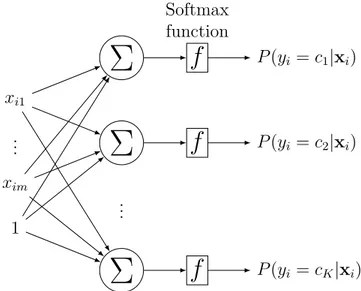
Consider now that we want to express the conditional probability distribution of the variable yi among the different classes, i.e., the K probabilities that xi belongs to each class ck. In
this context, a multi-class logistic regression generalizes Equation 2.5 as follows:
P (yi = ck|xi) =
exp(x>i wk)
PK
j=1exp(x>i wj)
= sof tmax(x>i wk) (2.6)
With wj = [wj0, wj1, ..., wjm] the weights associated with the jth class. Figure 2.2 illustrates
this process in a graphical form. Note that for the sake of readability, we did not represent the weights associated to each connection.
xi1 .. . xim 1
Σ
f
Softmax function P (yi = c1|xi)Σ
f
P (yi = c2|xi) .. .Σ
f
P (yi = cK|xi)Figure 2.2 Graph Representation of Multi-class Logistic Regression
It is interesting to remark that there are two ways of performing binary classification, i.e., yi ∈ {0, 1}. The first one consists in the operation illustrated in Figure 2.1 where the output
is one single real value: P (1|xi) using the sigmoid function. The second one considers binary
classification as a two-class classification problem which uses the softmax function to output a vector of two values: [P (0|xi), P (1|xi)].
2.2.2 Multi-layer Perceptron
A multi-layer perceptron (MLP) is a type of feed-forward artificial neural-network (ANN). ANNs, are a family of probabilistic models that can be seen as a mathematical abstraction of the biological nervous system. An ANN is composed of elementary units called “neurons”. As shown in Figure 2.3, an artificial neuron takes as input a set of numerical values. These input values are then summed and passed as input to an “activation function” that returns the output of the neuron.
Σ
f
Activation function Output Input 1 Input 2 .. .Figure 2.3 Graph Representation of an Artificial Neuron
There exists a variety of activation functions. As shown in Figure 2.4, most of them are step-like functions which reminds us of the behavior of a biological neuron, i.e., the neuron outputs a positive value only if the sum of the inputs is greater than a given threshold.
Figure 2.4 Examples of Activation Functions The architecture of a MLP model is organized as follows:
1. Neurons are organized in successive fully-connected layers (or dense layers), i.e., the output of a neuron is connected to all the neurons of the next layer and there exists no connections between neurons of a same layer.
2. Connections between neurons are weighted. Thus the input of a given neuron is a linear function of the outputs of all the neurons of the previous layer.
3. The input layer (i.e., the first layer) represents the attributes of the data used to perform classification.
4. The output layer (i.e., the last layer) represents the conditional probabilities for each label predicted by the model.
5. The hidden layers (i.e., the layers in between) have no direct connections with the environment.
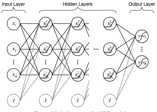
Let us illustrate such architecture with the MLP presented in Figure 2.5. This model takes as input m attributes and is composed of L hidden layers. It outputs a vector of K probabilities. We note Ml, l ∈ {1, 2, ..., L} the size (i.e., number of neurons) of the lth hidden layer.
Activation functions are represented inside the neurons. Here, hidden neurons have a relu activation function and the output neuron a softmax, thus outputting a probability.
Figure 2.5 Architecture of a MLP model
Note that input and hidden layers have an additional constant node called the bias. This node allows each neuron to receive as input a linear function of the output of the neurons of the previous layer. One can also remark that logistic regression is in fact equivalent to a MLP with no hidden layers.
2.2.3 Convolutional Neural Network
Convolutional Neural Networks are a special kind of feed-forward ANNs. These networks have proved to be extremely efficient to process multi-dimensional inputs such as images. Indeed, these networks happen to have a similar architecture than that of the human and animal visual cortex (Hubel and Wiesel (1962)). CNNs have originally been proposed by LeCun et al. (1998). However, their great potential for image processing have only been recognized by the community after the deep CNN proposed by Krizhevsky et al. (2012) achieved breakthrough results at the 2012 ImageNet Large Scale Visual Recognition Challenge (ILSVRC). CNNs are characterized by the use of successive so called convolution layers directly after the input layer. Then, the output of these convolution layers is usually fully-connected to a MLP model (i.e., dense layers).
Convolution Layer
A convolution layer takes as input a multi-dimensional array of numbers (typically an image) called a tensor and returns several filtered versions (called feature maps) of this input. There-fore, a convolution layer contains several fixed-size filters and outputs the filter’s response at each spatial location of the input. A convolution filter can be seen as an artificial neuron that takes as input a fixed-size portion of the input tensor and pass the weighted sum of its inputs to an activation function. Figure 2.6 illustrate the process of filtering of the input also called convolution. In this example, a 4 × 5 input tensor is filtered by a 1 × 2 convolution filter with a relu activation function, which produces a 4 × 4 output.
Pooling Layer
Once the input has been filtered by several filters, feature maps are often aggregated across a small spatial region to reduce their dimensionality. This process called pooling is usually done using the average or maximum value. Figure 2.7 illustrate a 2 × 2 max-pooling operation across the feature map presented in Figure 2.6.
Figure 2.7 2 × 2 max-pooling of a 4 × 4 feature map
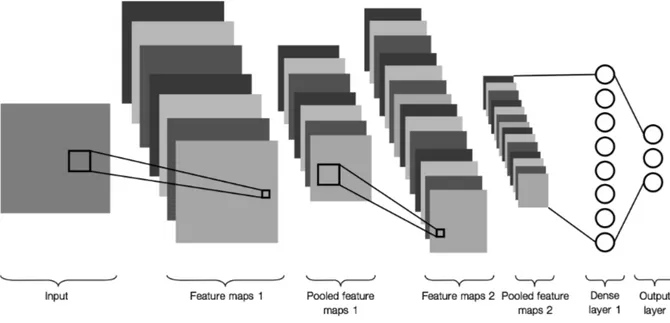
Thus, in a CNN, the input tensor is aggregated into several smaller tensors through multiple successive convolution + pooling operations. These output tensors are then flattened and concatenated to feed a MLP which performs the final prediction. Figure 2.8 overviews the whole process with a CNN composed of two convolution + pooling layers, one dense layer and three output neurons.
2.3 Optimization
The previous section focuses on the structure of the neural-networks used for classification. In this section, we address the problem of training such models, i.e., finding the set of weights that minimizes the error achieved by a model on a set of input–output examples. In the remainder of this section, we consider having a training set D = {(xi, yi)}ni=1 of instances
and their known associated labels. We note θ = {Wl}L+1l=1 the set of weights of the model we
want to train.
2.3.1 Loss Function
We have seen how neural networks map an input vector xi of real values into an output
vector f(xi, θ) of probabilities. Training a neural-network model, is the process of finding
an optimal set of weights θ∗ that minimizes the error (or loss) obtained by the model on the examples of D. Thus, one must define a loss function L(f(xi, θ), yi) that measures how
“bad” is the model’s prediction for a given example (xi, yi). Then, once the loss function is
defined, we want to minimize the mean loss performed by the model over every example of the training set, which is called the empirical risk:
θ∗ = argmin θ 1 N N X i=1 L(f(xi, θ), yi) (2.7)
There exists a variety of loss functions. The choice of the right loss to use for a given classification problem depends on the nature of this problem and how we want our model to behave. Equations 2.8 and 2.9 presents two commonly used loss functions, the cross entropy and the squared error :
cross_entropy = − K X k=1 [yiklog(fk(xi, θ)) + (1 − yik) log(1 − fk(xi, θ))] (2.8) squared_error = K X k=1 (fk(xi, θ) − yik)2 (2.9) 2.3.2 Gradient Descent
Gradient descent, is a procedure that allows to minimize the empirical risk by incrementally updating the model weights. At each epoch, i.e., pass over the whole training set, the weights are updated according to the gradient of the empirical risk computed with respect to the model weights. This process is repeated until the computed value of the empirical risk has
converged. Figure 2.9 shows the algorithm of gradient descent in pseudocode. The hyper-parameter η is called the learning rate. It represents the length of the step by which the weights are updated in the opposite direction to that of the gradient.
θ = θ0; // weights initialization
while converged == FALSE do
g = ∂ ∂θ[ 1 N N X i=1 L(f(xi, θ), yi)]; θ = θ − ηg; end
Figure 2.9 Gradient Descent Algorithm
In gradient descent, weights are only updated after all training examples have been fed through the model. However, weights can also be updated according to the gradient of the loss function computed for each training example, which is called stochastic gradient descent (SGD). Another variant of gradient descent called mini-batch stochastic gradient descent consists in splitting the training set in equal size subsets called mini-batch. Then, at each epoch, the training set is split into new mini-batches and the weights are updated according to the gradient of the empirical risk computed for each mini-batch.
2.3.3 Hyper-parameters Calibration
In the previous subsections, we have seen how to find an optimal set of weights θ∗ by incrementally updating θ according to the gradient of the loss. However, before training a neural-network, one must also find the optimal set of hyper-parameters for the model. For example, the number of layers in the network (L), the size of each layer (Ml) as well as the
learning rate (η) are common hyper-parameters that must be assessed before training. To do so, a common approach consists in keeping a portion of the training set (usually 30%) called the validation set to monitor the performances achieved by the model with different sets of hyper-parameters. Hence, for each set of hyper-parameters to test, the model is trained on the new training set (70%) and the performances are tested on the validation set (30%). Once the optimal set of hyper-parameters has been decided, it is a common practice to perform the final training of the model on the whole set (100%) to maximize the number of training examples. However, in this approach the validation set is selected randomly which can lead to a wrong choice of hyper-parameters if the 30% sample selected is not representative of the data. An alternative strategy is called the k-fold cross validation. It consists in splitting the training set into k equal size partitions called folds. Afterwards, each
set of hyper-parameters is tested k times by leaving one fold out for testing and keeping the remaining k − 1 for training. Finally, the performance value retained for the tested hyper-parameters is computed by taking the mean across the k generated values. Although k-fold cross validation usually leads to a better hyper-parameters calibration, it can be tedious to execute in practice, especially for deep-learning models that can take days to train.
The values of the hyper-parameters to test are usually selected using a random search, which simply consists in randomly selecting the value for each hyper-parameter inside a predefined range. This technique has proved to be more efficient than grid search (Bergstra and Bengio (2012)).
CHAPTER 3 LITERATURE REVIEW
During the past decade, the use of machine-learning has allowed great improvements in a variety of domains, and of course, the field of anti-patterns detection has not been immune from it. In this chapter, we first define the two anti-patterns considered in this thesis, then, we present a literature review of (1) conventional techniques used to detect these anti-patterns as well as their machine-learning counterparts and; (2) empirical studies conducted on the impact of anti-patterns on software systems.
3.1 Definitions
3.1.1 God Class
A God Class or Blob, is a class that tends to centralize most of the system’s intelligence, and implements a high number of responsibilities. It is characterized by the presence of a large number of attributes, methods and dependencies with data classes (i.e., classes only used to store data in the form of attributes that can be accessed via getters and setters). Thus, assigning much of the work to a single class, delegating only minor operations to other small classes causes a negative impact on program comprehension (Abbes et al. (2011)) and reusability. The alternative refactoring operation commonly applied to remove this anti-pattern is called Extract Class Refactoring and consists in splitting the affected God Class into several more cohesive smaller classes (Fowler (1999)).
3.1.2 Feature Envy
A method that is more interested in the data of another class (the envied class) than that of the class it is actually in. This anti-pattern represents a symptom of the method’s misplace-ment, and is characterized by a lot of access to foreign attributes and methods. The main consequences are an increase of coupling and a reduction of cohesion, because the affected method often implements responsibilities more related to the envied class with respect to the methods of its own class. This anti-pattern is commonly removed using Move Method Refactoring, which consists in moving all or parts of the affected method to the envied class (Fowler (1999)). Let us consider the situation where a class UseRectangle needs to compute the area of an instance of a class Rectangle. In the implementation presented in Figure 3.1, the class UseRectangle implements a method getArea(Rectangle) to compute the desired area from the public attributes provided by the class rectangle instead of asking the object
to do the computation himself. This is a clear case where the method getArea(Rectangle) envies the class Rectangle. As shown in Figure 3.2 this issue can be addressed by moving the envious method to the envied class thus keeping the attributes width and height private.
import Rectangle;
class UseRectangle {
private int area;
public UseRectangle(Rectangle r) {
this.area = getArea(r);
}
private int getArea(Rectangle r) {
int width = r.width;
int height = r.height;
return width*height;
} ... }
class Rectangle {
public int width;
public int height;
public Rectangle(int w, int h) {
this.width = w;
this.height = h;
} }
Figure 3.1 Feature Envy example
import Rectangle;
class UseRectangle {
private int area;
public UseRectangle(Rectangle r) {
this.area = r.getArea();
} ... }
class Rectangle {
private int width;
private int height;
public Rectangle(int w, int h) {
this.width = w; this.height = h; } public getArea() { return width*height; } }
3.2 Detection Techniques
The idea of anti-patterns or design smells has first been introduced by Webster (1995) to capture the pitfalls of object oriented development. Since then, number of books have been written to define new anti-patterns, sharpen the definition of existing ones, and propose alternative refactoring solutions. Among these books, Fowler (1999) wrote a taxonomy of 22 design and code smells and discussed that such smells are indicators of design or imple-mentation issues to be addressed by refactorings. Lanza and Marinescu (2007) provided a metric oriented approach to characterize, evaluate and improve the design of object oriented systems. Suryanarayana (2014) described 25 structural design smells contributing to tech-nical debt in software projects. Based on the definitions provided by these books, several automatic detection approaches have been proposed in the literature to detect instances of anti-patterns in source code. Later, as in many research fields, machine learning techniques have been used to overcome the performance issues encountered by the previous approaches. In the following, we present the detection approaches that have been proposed in literature to identify the occurrences of the two anti-patterns considered in this thesis.
3.2.1 God Class
Heuristic Based Detection Approaches
The first attempts to detect components affected by anti-patterns in general, and God Classes in particular have focused on the definition of rule-based approaches which use some metrics to capture deviations from good object oriented design principles. First, Marinescu (2004) presented detection strategy, a metric-based mechanism for analyzing source code models and detect design fragments using a quantifiable expression of a rule. They illustrate their methodology step by step by defining the detection strategy for God Class. Later, Lanza and Marinescu (2007) formulated their detection strategies for 11 design and code smells by de-signing a set of metrics for each smell along with thresholds. These metrics are combined with their respective thresholds to create the final detection rules for each anti-pattern. As de-scribed in Figure 3.3, God Class occurrences are detected using a set of three metrics, namely ATFD (Access To Foreign Data), WMC (Weighted Method Count), and TCC (Tight Class Cohesion). These heuristics have then been implemented to create anti-pattern detection tools like InCode (Marinescu et al. (2010)).
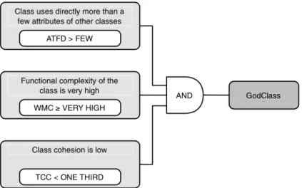
Similar to the approach described above, Moha et al. (2010) performed a systematic analysis of the definitions of code and design smells in the literature and proposed templates and a grammar to encode these smells and generate detection algorithms automatically. Based
Figure 3.3 Lanza and Marinescu (2007) detection rule for God Class.
on such analysis, they proposed the detection tool DECOR (DEtection and CORrection of Design Flaws), implemented for four design anti-patterns: God Class, Functional Decompo-sition, Spaghetti Code, and Swiss Army Knife, and their 15 underlying code smells. Their detection approach takes the form of a “Rule Card” which encodes the formal definition of anti-patterns and code smells. As described in Figure 3.4 the identification of classes affected by God Class is based on both structural and lexical information.
Figure 3.4 Moha et al. (2010) Rule Card for God Class detection. (Hexagons are anti-patterns, gray ovals are code smells, and white ovals are properties).
Other approaches rely on the identification of refactoring opportunities to detect anti-patterns. Based on this consideration, instances of a given anti-pattern can be detected in a system by looking at the opportunities to apply the corresponding refactoring operation. In this context, Fokaefs et al. (2012) proposed an approach to detect God Classes in a system by suggesting a set of Extract Class Refactoring operations. This set of refactoring
opportu-nities is generated in two main steps. First, they identify cohesive clusters of entities (i.e., attributes and methods) in each class of the system, that could then be extracted as separate classes. To do so, the Jaccard distance is computed among each class members (i.e., entities). The Jaccard distance between two entities ei and ej measures the dissimilarity between their
respective “entity sets” Si and Sj and is computed as follows:
dist(ei, ej) = 1 −
|Si∩ Sj|
|Si∪ Sj|
(3.1)
For a method, the “entity set” contains the entities accessed by the method, and for an attribute, it contains the methods accessing the attribute. Then, cohesive groups of entities are identified using a hierarchical agglomerative algorithm on the information previously generated. In the second step, the potential classes to be extracted are filtered using a set of rules, to ensure that the behavior of the original program is preserved. Later, this approach has been implemented as an Eclipse plug-in called JDeodorant (Fokaefs et al. (2011)). The approaches described above are solely based on structural information to predict whether an entity is affected of not by an anti-pattern. However, anti-patterns can also impact how source code entities change together over time. Based on such considerations, Palomba et al. (2013, 2015a) proposed HIST (Historical Information for Smell deTection), an approach to detect anti-patterns occurrences in systems using historical information derived from ver-sion control systems (e.g., Git, SVN). They applied their approach to the detection of five anti-patterns: Divergent Change, Shotgun Surgery, Parallel Inheritance, God Class and Fea-ture Envy. The detection process followed by HIST consists of two steps. First, historical information is extracted from versioning systems using a component called change history extractor which outputs the sequence of changes applied to source code entities (i.e., classes or methods) through the history of the system. Second, a set of rules is applied to this so produced sequence to identify occurrences of anti-patterns. In this context, God Classes are identified as: “classes modified (in any way) in more than α% of commits involving at least another class”, with a value of α set to 8% after parameter calibration.
Machine-learning Based Detection Approaches
The approaches described above detect God Classes among other classes of a system using manually-defined heuristics, while a number of machine-learning based approaches have been proposed in the past decade. First, Kreimer (2005) proposed the use of decision trees to identify occurrences of God Class and Long Method. Their model relies on the number of fields, number of methods, and number of statements as decision criteria for God Class
detection and have been evaluated on two small systems (IYC and WEKA). This observation has been confirmed 10 years later by Amorim et al. (2015) who extended this approach to 12 anti-patterns.
Khomh et al. (2009a, 2011) presented BDTEX (Bayesian Detection Expert), a metric based approach to build Bayesian Belief Networks from the definitions of anti-patterns. This ap-proach has been validated on three different anti-patterns (God Class, Functional Decompo-sition, and Spaghetti Code) and provides a probability that a given entity is affected instead of a boolean value like other approaches. Following, Vaucher et al. (2009) relied on Bayesian Belief Networks to track the evolution of the“godliness” of a class and thus, distinguishing real God Classes from those that are so by design.
Later, Maiga et al. (2012a,b) introduced SVMDetect, an approach based on Support Vector Machines to detect four well known anti-patterns: God Class, Functional Decomposition, Spaghetti code, and Swiss Army Knife. The input vector fed into their classifier for God Class detection is composed of 60 structural metrics computed from the PADL meta-model (Guéhéneuc (2005)).
Fontana et al. (2016) performed the largest experiment on the effectiveness of machine learn-ing algorithms for smell detection. They conducted a study where 16 different machine learning algorithms were implemented (along with their boosting variant) for the detection of four smells (Data Class, God Class, Feature Envy, and Long Method) on 74 software sys-tems belonging to the Qualitas Corpus dataset (Tempero et al. (2010)). The experiments have been conducted using a set of independent metrics related to class, method, package and project level as input information and the datasets used for training and evaluation have been filtered using an under-sampling technique (i.e., instances have been removed from the original dataset) to avoid the poor performances commonly reported from machine learning models on imbalanced datasets. Their study concluded that the algorithm that performed the best for God Class detection was the J48 decision tree algorithm with an F-measure of 99%. However, Di Nucci et al. (2018) replicated their study and highlighted many limitations. In particular, the way the datasets used in this study have been constructed is strongly discussed and the performances achieved after replication were far from those originally reported.
3.2.2 Feature Envy
Heuristic Based Detection Approaches
As for other anti-patterns, the first approaches proposed to detect Feature Envy are based on manyally-defined heuristics that rely on some metrics. First, Lanza and Marinescu (2007)
proposed the detection strategy illustrated in Figure 3.5 which rely on: (1) the number of Accesses To Foreign Data (ATFD) made by a method; (2) the Locality of Attribute Accesses (LAA), i.e., ratio between the number of accesses to attributes that belongs to the envied class vs. the enclosing class and; (3) the number of Foreign Data Providers (FDP) i.e., the number of classes accessed in the body of a method. One must remark that this approach focuses only on predicting whether or not a method is involved in the Feature Envy anti-pattern but does not provide any information about the envied class.
Figure 3.5 Lanza and Marinescu (2007) detection rule for Feature Envy.
Similarly to this work, Nongpong (2015) proposed the Feature Envy Factor, a metric for automatic Feature Envy detection. This approach relies on counting the number of calls made on a given object by the method under investigation, in order to produce a metric assess from zero to one how good is the Feature Envy candidate. The Feature Envy Factor between an object obj and a method mtd is computed as follows:
F EF (obj, mtd) = w(m/n) + (1 − w)(1 − xm) (3.2) Where m is the number of calls on the object obj; n is the total number of calls on any objects defined or visible by the method mtd; w and x are real values in the range [0, 1]. It is also possible to detect occurrences of Feature Envy by looking at the opportunities to apply the corresponding refactoring operation. Methods that can potentially be moved to another class under certain conditions are presented to the software engineer as potentially affected components. In this context, Tsantalis and Chatzigeorgiou (2009) proposed an ap-proach for automatic suggestions of Move Method Refactoring. First, for each method m in the system, a set of candidate target classes T is created by examining the entities that are accessed in the body of m. Second, T is sorted according to two criteria: (1) the number of
entities that m accesses from each target class of T in descending order and; (2) the Jaccard distance from m to each target class in ascending order if m accesses an equal number of entities from two or more classes. In this context, the Jaccard distance between an entity e and a class C is computed as follows:
dist(e, C) = 1 −|Se∩ SC| |Se∪ SC| where Sc= [ e∈C {e} (3.3)
With Se the entity set of a method defined in Equation 3.1. Third, T is filtered under the
condition that m must modify at least one data structure in the target class. Fourth, they suggest to move m to the first target class in T that satisfies a set of preconditions related to compilation, behavior, and quality. This algorithm is implemented in the Eclipse plug-in JDeodorant (Fokaefs et al. (2007)).
Similarly to God Class, Palomba et al. (2013, 2015a) proposed to detect Feature Envy using historical information. First, the sequence of co-changed methods is extracted from version control systems using the Change History Extractor. Then, the detection rule for HIST rely on the conjecture that “a method affected by feature envy changes more often with the envied class than with the class it is actually in”. Thus, Feature Envy methods are identified as those involved in commits with methods of another class of the system β % more than in commits with methods of their class. The value of β being set to 80% after parameter calibration.
Machine-learning Based Detection Approaches
The first attempt to detect Feature Envy using machine-learning techniques has been pro-posed by Fontana et al. (2016) during their large-scale study. In this context, the J48 decision tree algorithm outperformed other classifiers in detecting Feature Envy with an F-measure of 97%. Again, these results have been challenged by Di Nucci et al. (2018).
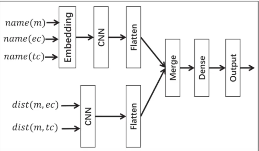
More recently, Liu et al. (2018) proposed a deep learning based approach to detect Feature Envy. Their approach relies on both structural and lexical information. On one side, the names of the method, the enclosing class (i.e., where the method is implemented) and the envied class are fed into convolutional layers. On the other side, the distance proposed by Tsantalis and Chatzigeorgiou (2009) is computed for both the enclosing class (dist(m, ec)) and the target class (dist(m, tc)), and values are fed into other convolutional layers. Then the output of both sides is fed into fully-connected layers to perform final decision. To train and evaluate their model, they use an approach similar to Moghadam and Cinneide (2012) where labeled samples are automatically generated from open-source applications by the injection of affected methods. These methods assumed to be correctly placed in the original systems
are extracted and moved into random classes to produce artificial Feature Envy instances (i.e., misplaced methods). Figure 3.6 overviews the proposed approach.
Figure 3.6 Liu et al. (2018) architecture for Feature Envy detection.
3.3 Empirical Studies on Anti-patterns
This section reports the empirical studies that have been conducted on anti-patterns. First we present studies aiming to understand the impact of anti-patterns on software quality. Second, we overview the studies conducted to understand how anti-patterns appear and evolve over time.
3.3.1 Impact of Anti-patterns on Software Quality
First, Deligiannis et al. (2004) performed a controlled experiment to understand the impact of God Class on design quality. Their results show that the presence of God Classes in a system negatively impacts the maintainability of the source code. Furthermore they concluded that it considerably impacts the way developers apply the inheritance mechanism. Yamashita and Moonen (2012) investigated the relation between specific anti-patterns and a variety of maintenance characteristics such as effort, change size and simplicity. They identify which anti-patterns can be used as indicator for maintainability assessments based on: (1) expert-based maintainability assessments of four Java systems and; (2) observations and interviews with professional developers who were asked to maintain these systems during a period of time. For the anti-patterns considered in this thesis, their results show that God Class affects the Simplicity and the Use Of Components and that Feature Envy affects the Logic Spread. Later Yamashita and Moonen (2013) performed a similar study aiming at understanding the
interactions between co-located anti-patterns and the impact of such interactions on software maintenance.
Abbes et al. (2011) conducted an empirical study with the aim of understanding the impact of two anti-patterns, namely God Class and Spaghetti Code on program comprehension. In this study, subjects were asked to perform basic tasks related to program comprehension on systems affected or not by the investigated anti-patterns. The results of their study show: (1) an increase in subjects’ time and effort and a decrease of their percentage of correct answers in systems affected by God Class; (2) no significant correlation between program comprehension and the presence of Spaghetti Code and; (3) a strong difference between subjects’ efforts, times, and percentages of correct answers on systems affected by both anti-patterns.
Khomh et al. (2009b, 2012) conducted a large scale empirical study investigating the relation between the presence of anti-patterns and the classes change- and fault-proneness. They investigate 13 anti-patterns in 54 releases of four software systems and analyze the changes and fault-fixing operations applied to the classes of these systems. Their results indicate clearly that classes participating in anti-patterns are more change- and fault-prone than classes not affected by any anti-pattern. Later, Palomba et al. (2018) confirmed the above findings by performing a similar experiment on a larger number of systems.
3.3.2 Evolution and Presence of Anti-patterns
First, Olbrich et al. (2009) studied the impact of anti-patterns on the change behavior of code components. Specifically, they analyzed the historical data over several years of devel-opment, of two large scale software systems and compared the change frequency and size of components affected by God Class and Shotgun Surgery with those of healthy components. With the results of their study, the authors confirmed that affected components exhibit dif-ferent change behaviors. They also identified difdif-ferent phases in the life of software systems where the number of anti-patterns increase and decrease. Similarly, Vaucher et al. (2009) studied the “life cycle” of God Class occurrences in two open-source systems with the aim of understanding when they arise and how they evolve. With the results of their study, the authors were able to develop prevention mechanisms to predict whether changes applied to the system are likely to introduce new anti-patterns.
On the same line, Chatzigeorgiou and Manakos (2010) tracked the evolution of three anti-patterns: Long Method, Feature Envy and State Checking in the history of two open-source systems, showing that: (1) anti-patterns persist after being introduced; (2) most of the time, anti-patterns are introduced when the component they affect is added to the system and; (3) few occurrences are willingly removed through refactoring operations.
Tufano et al. (2015) performed the largest experiment on the presence of anti-patterns through the history of systems. Specifically, they mined the history of 200 software projects to understand when and why (i.e., under what circumstances) anti-patterns appear. First, their results confirm the observation made by Chatzigeorgiou and Manakos (2010) that most of instances are introduced when the file is added to the system. Second, they show that anti-patterns are also often introduced the last month before deadlines by experienced devel-opers.
Finally, Palomba et al. (2018) assessed during their large scale study, the diffuseness, i.e., the percentage of affected code components of 13 anti-patterns in 30 open-source systems. They concluded that most of the anti-patterns are quite diffused, especially the ones characterized by their size or complexity. However they also identified few other anti-patterns such as Feature Envy that are less diffused.
CHAPTER 4 STUDY BACKGROUND
This chapter presents the background common to the studies detailed in the remainder of this thesis. First, we present and discuss the choice of the eight software systems considered in these studies. Second, we describe the oracle we created to conduct our experiments, which reports the occurrences of God Class and Feature Envy in the studied systems. Third, we overview the metrics used for evaluation. Finally, we discuss the considerations adopted to train machine-learning models on the task of anti-patterns detection.
4.1 Studied Systems
The context of our studies consists of eight open-source Java software systems belonging to various ecosystems. Two systems belong to the Android APIs1: Android Opt Telephony and
Android Support. Four systems belong to the Apache Foundation2: Apache Ant, Apache
Tomcat, Apache Lucene, and Apache Xerces. Finally, one free UML design software: Ar-goUML3and one text editor: Jedit4available under GNU General Public License5. As further
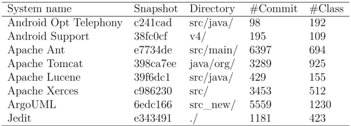
discussed in Section 4.2, this choice is motivated by the preliminary manual-detection of God Classes performed in prior studies on these systems (Moha et al. (2010); Palomba et al. (2013)). Without loss of generalizability, we chose to analyze only the directories that im-plement the core features of the systems and to ignore test directories. Table 4.1 reports for each system, the Git identification (SHA) of the considered snapshot, its “age” (i.e., number of commit) and its size (i.e., number of class).
Table 4.1 Characteristics of the Studied Systems
System name Snapshot Directory #Commit #Class Android Opt Telephony c241cad src/java/ 98 192
Android Support 38fc0cf v4/ 195 109
Apache Ant e7734de src/main/ 6397 694
Apache Tomcat 398ca7ee java/org/ 3289 925
Apache Lucene 39f6dc1 src/java/ 429 155
Apache Xerces c986230 src/ 3453 512
ArgoUML 6edc166 src_new/ 5559 1230
Jedit e343491 ./ 1181 423 1https://android.googlesource.com/ 2https://www.apache.org/ 3http://argouml.tigris.org/ 4http://www.jedit.org/ 5https://www.gnu.org/
4.2 Building a Reliable Oracle
To train and evaluate the performances of our models, we needed an oracle reporting the occurrences of the studied anti-patterns in the considered systems snapshots. We found no such large dataset in the literature. One existing crowd-sourcing dataset, Landfill created by Palomba et al. (2015b) included manually-produced anti-pattern instances but we found many erroneously-tagged instances, which discouraged and prevented its use in our work. For God Class, we found two sets of manually-detected occurrences in open-source Java sys-tems, respectively from DECOR (Moha et al. (2010)) and HIST (Palomba et al. (2013)) replication packages. Thus, we created our oracle from these occurrences under two con-straints: (1) the full history of the system must be available and (2) the occurrences reported must be relevant. After filtering, over the 15 systems available in these replication packages, we retained eight to construct our oracle.
For Feature Envy, most of the approaches proposed in the literature are evaluated on artifi-cial examples, i.e., assuming methods are correctly placed in the original systems, they are extracted and moved into random classes to produce Feature Envy occurrences (i.e., mis-placed methods) (Moghadam and Cinneide (2012); Sales et al. (2013); Liu et al. (2018)). However, our approach relies on the history of code components. Therefore, such artificial anti-patterns are not usable because they have been willingly introduced in the considered systems’ snapshot. Thus, we had to build manually our own oracle.
First, we formed a set of 779 candidate Feature Envy instances over the eight subject systems by merging the output of three detection tools (HIST, InCode, and JDeodorant), adjusting their detection thresholds to produce a number of candidate per system proportional to the systems sizes. Second, three different groups of people manually checked each candidate of this set: (1) the author of this thesis, (2) nine M.Sc. and Ph.D. students, and (3) two software engineers. We gave them access to the source code of the enclosing classes (where the methods were defined) and the potential envied classes. After analyzing each candidate, we asked respondents to report their confidence in the range [strongly_approve, weakly_approve, weakly_disapprove, strongly_disapprove]. To avoid any bias, none of the respondent was aware of the origin of each candidate. We made the final decision using a weighted vote over the reported answers. First we assigned the following weights to each confidence level:
strongly_approve → 1.00 weakly_disapprove → 0.33 weakly_approve → 0.66 strongly_disapprove → 0.00
Then, an instance is considered as a Feature Envy if the mean weight of the three answers reported for this instance is greater than 0.5.
Table 4.2 reports, for each system, the number of God Classes, the number of produced candidate Feature Envy instances, and the number of Feature Envy instances retained after manual-validation.
Table 4.2 Characteristics of the Oracle
System name #God_Class #Candidate_FE #Feature_Envy
Android Opt Telephony 11 62 18
Android Support 4 21 2 Apache Ant 7 110 25 Apache Tomcat 5 173 57 Apache Lucene 4 42 4 ArgoUML 22 144 24 Jedit 5 98 22 Xerces 15 129 37 Total 73 779 189 4.3 Evaluation Metrics
To compare the performances achieved by different approaches on the studied systems, we consider each approach as a binary classifier able to perform a boolean prediction on each entity of the system. Thus, we evaluate their performances using the following confusion matrix:
Table 4.3 Confusion Matrix for Anti-patterns Detection
predicted total 1 0 true 1 A B npos 0 C D nneg
total mpos mneg n
With (A) the number of true positives, (B) the number of misses, (C) the number of false alarms and (D) the number of true negatives. Then, based on this matrix, we compute the widely adopted precision and recall metrics:
precision = A
A + C (4.1) recall =
A
A + B (4.2) We also compute the F-measure (i.e., the harmonic mean of precision and recall) to obtain a single aggregated metric:
F -measure = 2 × precision × recall
precision + recall = 2 ×
A npos+ mpos
4.4 Training
This section discusses the considerations adopted to train neural-networks on the task of anti-patterns detection. We consider training a multi-layer feed-forward neural-network to perform a boolean prediction on each entity of the training systems. First, the training set contains N training systems which can be expressed as:
D = {Si}Ni=1, with Si = {(xijyij)}nj=1i (4.4)
With Si the ith training system, xij the input vector corresponding to the jth entity of this
system, yij ∈ {0, 1} the true label for this entity and ni the size (i.e., number of entities) of
Si. Second, we refer to the output of the neural network corresponding to the positive label,
i.e., the predicted probability that an entity is affected as: Pθ(1|xij).
4.4.1 Custom Loss Function
Software systems are usually affected by a small proportion of anti-patterns (< 1%) (Palomba et al. (2018)). As a consequence, the repartition of labels within a dataset composed of software system entities is highly imbalanced. Such imbalanced dataset compromises the performances of models optimized using conventional loss functions (He and Garcia (2008)). Indeed, the conventional binary_cross_entropy (cf. Equation 2.8) loss function maximizes the expected accuracy on a given dataset ,i.e., the proportion of instances correctly labeled. In the context of anti-patterns, the use of this loss function lead to useless models that assign the majority label to all input instances, thus maximizing the overall accuracy (> 99%) during training. To overcome this issue, we must define a loss function that reflects our training objective (i.e., maximizing the F-measure achieved over the training systems). Let us formulate our training objective as finding the set of parameters θ∗ that maximizes the mean F-measure achieved over the training system, which can be expressed as:
θ∗ = argmax θ 1 N N X i=1 Fm(θ, Si) (4.5)
Which is equivalent to the minimization of the empirical risk expressed in Equation 2.7 with a loss: L = −Fm. However, to solve this problem through gradient descent, we need our loss
to be a continuous and differentiable function of the weights θ. As defined in Equation 4.3, the F-measure does not meet this criterion, which prevents its direct use to define our loss function. Indeed, computing the number of true positives (A) and positives (mpos) requires