an author's https://oatao.univ-toulouse.fr/26818
https://doi.org/10.1049/iet-rsn.2020.0168
Medina, Daniel and Ortega, Lorenzo and Vilà-Valls, Jordi and Closas, Pau and Vincent, Francois and Chaumette, Eric Compact CRB for delay, Doppler, and phase estimation – application to GNSS SPP and RTK performance
Compact CRB for delay, Doppler, and phase
estimation – application to GNSS SPP and
RTK performance characterisation
doi: 10.1049/iet-rsn.2020.0168Daniel Medina
1, Lorenzo Ortega
2, Jordi Vilà-Valls
3, Pau Closas
4, Francois Vincent
3, Eric Chaumette
3 1Institute of Communications and Navigation, German Aerospace Center (DLR), Neustrelitz, Germany2Telecommunications for Space and Aeronautics Lab (TéSA), Toulouse, France 3ISAE-SUPAERO, University of Toulouse, Toulouse, France
4Department of Electrical and Computer Engineering, Northeastern University, Boston, MA, USA
E-mail: [email protected]
Abstract: The derivation of tight estimation lower bounds is a key tool to design and assess the performance of new estimators.
In this contribution, first, the authors derive a new compact Cramér–Rao bound (CRB) for the conditional signal model, where the deterministic parameter's vector includes a real positive amplitude and the signal phase. Then, the resulting CRB is particularised to the delay, Doppler, phase, and amplitude estimation for band-limited narrowband signals, which are found in a plethora of applications, making such CRB a key tool of broad interest. This new CRB expression is particularly easy to evaluate because it only depends on the signal samples, then being straightforward to evaluate independently of the particular baseband signal considered. They exploit this CRB to properly characterise the achievable performance of satellite-based navigation systems and the so-called real-time kinematics (RTK) solution. To the best of the authors’ knowledge, this is the first time these techniques are theoretically characterised from the baseband delay/phase estimation processing to position computation, in terms of the CRB and maximum-likelihood estimation.
1 Introduction
Time-delay estimation has been a research topic of significant interest in many fields such as radar, sonar, communications, and navigation [1–6], to name a few, mainly because this drives the first stage of the receiver to localise and track radiating sources [7]. In addition, phase estimation is also a fundamental part in many applications, for instance, global navigation satellite systems (GNSS) precise navigation approaches rely on the exploitation of the signal phase information. Indeed, the phase measurement is linked to the wavelength, which in this case is much smaller than the baseband signal resolution. This is also the case in precise GNSS remote sensing altimetry applications [8–10], where the phase must be exploited to achieve cm altimetric precision. In a broader perspective, these applications typically deal with complex circular observation vectors [11]. Within this class, an important estimation problem is the identification of the components of a noisy observation vector x formed from a linear superposition of Q sources α in noise w [12–15]
x= A η α + w, x, w ∈ ℂN, A η ∈ ℂN×Q, α ∈ ℂQ, (1)
where the mixing matrix A(η) depends on an unknown deterministic parameter vector η∈ ℝP, with N, Q the number of
samples and sources, respectively. Within the framework of modern array processing [11, 15] two different signal models are considered: the conditional signal model (CSM) and the unconditional signal model [13]. We adopt the less constrained CSM framework. Finding the relationship between the baseband CSM used in GNSS and the performance of GNSS positioning techniques ignited this contribution.
1.1 From multi-source to single source estimation
The analogue side of a classical GNSS receiver architecture includes a low noise amplifier, and a down-conversion to an intermediate sampling frequency Fs, followed then by an
analogue-to-digital converter. At this stage, one works with a multi-source signal as (1), e.g. data samples from all the signal types
broadcasted by the satellites in view. Owing to the similar incoming energy and low cross-correlation among GNSS signals, the multiple signals can be easily split into single source CSMs. The estimation of single source CSM and its relation to the performance of GNSS positioning techniques is, in turn, the main focus of this work.
Despite nearly optimal properties (in the asymptotic regime, i.e. in the large sample regime [13] and/or high signal-to-noise (SNR) regime [16]) of conditional maximum likelihood estimators (CMLEs) on CSMs, these estimators suffer from a large computational cost, as they typically require solving a non-linear multidimensional (possibly high-dimensional) optimisation problem. To circumvent this problem, several suboptimal techniques have been introduced: (i) substituting the multidimensional search with a simpler one-dimension search, e.g. Capon or MUSIC methods [17], (ii) restricting to a single source search, e.g. CLEAN [18] or alternating projection algorithms [19], or (iii) exploiting the extended invariance principle (EXIP) [20], which is based on a re-parameterisation of the problem that simplifies the maximum likelihood (ML) criterion to be maximised. In EXIP, the efficiency property of the original ML is maintained (at least asymptotically) through a weighted least square (WLS) refinement step by using a matched weighting matrix. The EXIP approach has been used in array [21] and/or radar [22] processing applications, and more recently in the context of GNSS [23].
In GNSS, the EXIP applied to the ML direct position estimation (DPE) [24, 25] leads to the widespread suboptimal two-step positioning approach, with the aim of providing position, velocity and time (PVT) estimates: (i) first, the delay and Doppler for each satellite-to-receiver link are estimated independently and then (ii) delay and Doppler estimates are translated into the so-called pseudo-range and pseudo-range rate observations, the latter fused to obtain the user PVT thanks to a WLS minimisation. In standard GNSS receivers, these two steps are typically done sequentially and the use of pseudo-range and pseudo-range rate measurements is not directly linked to the baseband signal processing, i.e. delay/ Doppler estimation are an input to the WLS, and their corresponding covariances set somehow empirically, sometimes
based on the satellite elevation or the estimated carrier-to-noise density (C/N0) at the receiver [26–28]. The optimal estimation performance of the WLS stage can only be assessed if the performance of the first synchronisation stage is optimally determined. It is thus of the utmost importance to characterise asymptotic performance of such CMLE first step associated with the single source CSM
x= a(η)α + w, x, w ∈ ℂN, a(η) ∈ ℂN, α ∈ ℂ . (2a)
The CMLE's asymptotic performance in the mean-square-error (MSE) sense is accurately described by the Cramér–Rao bound (CRB). So, it is not surprising that several CRB expressions for the single source estimation problem have been derived, for finite [29– 33] or infinite [34] bandwidth signals, where the starting point is often either the Slepian–Bangs formulas [35] or general theoretical CRB expressions for Gaussian observation models [15, 17, 36].
When the use of GNSS precise positioning approaches are required (i.e. in intelligent transportation systems or safety-critical applications [37]), such as the so-called real-time kinematics (RTK) [38, Ch. 26] or precise point positioning techniques [38, Ch. 25], the solution involves exploiting, together with delay and Doppler, the signal phase information as well. As a consequence, with respect to (w.r.t.) the single source CSM in (2a), in addition to
η, precise positioning requires estimation of the signal amplitude
and phase, and thus the following reparameterisation can be used
x= a(η)ρejφ+ w, x, w ∈ ℂN, a(η) ∈ ℂN, ρ ∈ ℝ+. (2b)
To the best of our knowledge, no compact CRB formula for the joint estimation of ε⊤= (σ
w2, ρ, φ, η⊤), where σw2 is the power of the
white noise vector w (such that w∼ CN(0, σw2IN)), seems to be
available in the open literature [13–15, 17, 29–36, 39–46]. Only by assessing the performance of CMLE at the single source CSM, the stochastic modelling of PVT observables can be determined.
1.2 Contributions
• The derivation of a new compact CRB for the general CSM in (2b) is provided in Section 4. A noteworthy feature of the new compact CRB is its ease-of-use for problems where the CRBs
on η and α (complex amplitude instead of amplitude and phase)
have already been computed.
• The particularisation of the compact CRB for the general CSM for the GNSS narrowband signal model is presented. Such CRB constitutes the extension of the preliminary results in [47], where a CRB for time-delay estimation under constant transmitter-to-receiver propagation delay (i.e. no Doppler effect and static scenario) was considered. In this contribution, the more comprehensive case of joint delay, Doppler, phase, and amplitude estimation is considered, with the corresponding CRB being derived in Section 5. Indeed the general problem is encountered in a multitude of applications, therefore, a tractable CRB for this problem constitutes a key tool of broad interest. The new CRB is obtained for the standard narrowband signal model, where the Doppler effect on the band-limited baseband signal is not considered and amounts to a frequency shift.
• The CRB is expressed in terms of the signal samples, making it especially easy to use irrespective of the considered baseband signal such that the actual sample values are used.
• Leveraging recent results on the CRB for a mixture of real- and integer-valued parameter vectors [48], summarised in Section 6 for completeness, we exploit both CRBs to properly characterize the ultimate GNSS single point positioning (SPP) and RTK performance. To the best of our knowledge, this is the first time, these positioning techniques are theoretically characterised from the baseband signal model in terms of the CRB and CMLE. Important findings are (i) the achievable SPP performance with large GNSS bandwidth signals, and the corresponding receiver operation point which allows reaching the PVT asymptotic behaviour, and (ii) the impact of such GNSS signals in the RTK asymptotic behaviour and the CMLE threshold region. Pictorial support for the narrowband CSM to PVT performance characterisation is provided in Fig. 1.
1.3 Notation and organisation
The notation convention adopted is as follows: scalars, vectors, and matrices are represented, respectively, by italic, bolditalic lowercase, and bolditalic uppercase characters. The scalar/matrix/ vector transpose and conjugate transpose are indicated by the superscripts ( ⋅ )⊤ and ( ⋅ )H. I is the identity matrix. A B and A
B
denote the matrix resulting from the horizontal and vertical concatenation of A and B, respectively. Re( ⋅ ) and Im( ⋅ ) refer to the real and imaginary parts. ∥ ⋅ ∥ describes an Euclidean norm and the norm w.r.t. A is ∥ ⋅ ∥A = ( ⋅ )⊤A−1( ⋅ ). tr( ⋅ ) represents the
trace operator and diag( ⋅ ) refers to a diagonal matrix whose entries are given by ( ⋅ ).
The paper is organized as follows. The narrowband signal model is detailed in Section 2, and both SPP and RTK are introduced in Section 3. The new CRB for the generic CSM is given in Section 4. The CRB for the joint delay, Doppler, phase, and amplitude estimation for narrowband signals is derived in Section 5. The main results for the mixed real-integer parameters CRB [48] are summarised in Section 6. Finally, a complete discussion on the GNSS SPP and RTK performance is given in Section 7. Conclusion and final remarks are drawn in Section 8.
2 Standard narrowband signal model
Given a generic band-limited signal c(t) with bandwidth B (for instance, it can represent the so-called pseudo-random noise (PRN) code in the GNSS terminology), it can be expressed in time and frequency as c t =
∑
n = N1 N2 c nTssinc πFst − nTs ⇌ c f = Ts∑
n = N1 N2 c nTse−j2πnTs1− B2,B2( f ) (3a)where Fs≥ B, c n Ts are the samples of c t , N1, N2∈ ℤ, N1≤ N2,
and ⇌ refers to the time-frequency pair. We consider the
Fig. 1 Overview of the contribution for the PVT (i.e. SPP and RTK) performance characterisation. From the narrowband CSM, the compact CRBs for
time-delay, Doppler, phase, and amplitude estimation are derived. From these signal model unknown parameters, GNSS code and phase observations are obtained and fed to the PVT estimator. Then, the CRB and the ML estimates for SPP and RTK are discussed and the overall positioning performance is addressed in direct relation to the sampling frequency and SNR
IET Radar Sonar Navig., 2020, Vol. 14 Iss. 10, pp. 1537-1549
transmission of this band-limited signal c t over a carrier
frequency fc (such that λc= c/ fc, with c the speed of light in
vacuum), from transmitter T to receiver R. Both transmitter and receiver are in uniform linear motion: their respective positions evolve as pT(t) = pT+ vTt and pR(t) = pR+ vRt, where p and v
represent the corresponding position and velocity vectors. In this context, we tackle the case where the propagation delay τ0t due to
the relative radial movement between T and R can be approximated, during the observation time, by a first-order distance-velocity model
∥ pTRt ∥ ≜ ∥ pTt − τ0t − pRt ∥
= cτ0t ≃ d + vt ⇒ τ0t ≃ τ + bt, τ = dc, b = vc,
(3b) where d is the T-to-R relative radial distance, v is the T-to-R relative radial velocity, and b is a delay drift related to the Doppler effect.
This so-called relative uniform radial movement is characterised by the time-delay τ due to the propagation path and
the dilation (1 − b) induced by the Doppler effect. Under the narrowband hypothesis, i.e. B ≪ fc, the Doppler effect on the band-limited baseband signal c t may be considered negligible: c (1 − b)(t − τ) ≃ c t − τ . In this case, for an ideal transmitter,
propagation channel, and receiver, the signal at the output of the receiver's Hilbert filter (I/Q demodulation, bandwidth Fs) is well approximated as [29, (2.1)] [33, (3)] x t ≜ x t; η = αc t − τ e−jωcb t−τ + w t , Rwτ = σw2sinc πFsτ ⇌ Rw f = σw 2 Fs, f ∈ −F2 ,s F2s (3c)
where ωc= 2π fc, η⊤= τ, b , and α is a complex amplitude that
includes all the transmission budget terms. The Fourier pair
Rwτ ⇌ Rw f is the model for the correlation function and the
power spectrum density of white noise over the band Fs. If we consider the acquisition of N′ = N2′ − N1′ + 1 (N1′ ≪ N1, N2′ ≫ N2)
samples at Ts= 1/Fs, then the discrete vector signal model is given
by (2a), or equivalently (2b), with
x= a(η)ρejφ+ w, ρ ∈ ℝ+, 0 ≤ φ ≤ 2π, x⊤= (…, x(n′T s), …), a⊤(η) = (…, c(n′T s− τ)e−jωcb(n′Ts −τ), …), w⊤= (…, w(n′Ts), …), (3d)
for N1′ ≤ n′ ≤ N2′ (dimension N′). We also define
c⊤≜ (…, c(nT
s), …), for N1≤ n ≤ N2 (dimension N). Notice that c(t) can be directly a PRN code with a binary phase shift keying
(BPSK) modulation where there is no subcarrier, as in the case of the global positioning system (GPS) L1 C/A signal, or a subcarrier modulated PRN, i.e. using a binary offset carrier [49] type modulation such as in the modernised GPS L1 C or Galileo E1 Open Service signals. The subcarrier has a direct impact on the correlation function, therefore on the estimation performance. On top of that, the signal may have data bits or not, depending on if it belongs to a data component or a pilot component.
3 GNSS SPP/RTK problem formulation
3.1 GNSS baseband signal processing
As already stated, using the EXIP principle within the ML DPE [24] leads to the standard GNSS two-step positioning approach [23]. The first step relies on the CMLEs of delay, Doppler, and phase for each individual satellite, which are expressed as
η= arg max η a Hη a η −1 aHη x2 , (4a) φ η = arg aHη a η −1 aHη x . (4b)
Notice that the phase CMLE is given by the argument of the cross-ambiguity function evaluated at the delay and Doppler CMLEs. Then, if the delay-Doppler CMLE reached its asymptotic performance so does the phase estimate.
3.2 GNSS code and phase observables
From the delay and phase CMLEs introduced in Section 3.1, together with the navigation data demodulation, one constructs the so-called code and phase observables. More precisely, we are interested in the pseudo-range ϱi and phase Φi observables, which
for the ith satellite are modelled as
ϱi= cτi= ∥ pTi− pR∥ + c δtr− δti +cδtiiono+ cδtitrop+ ϵϱ,i, (5) Φi= 2πφλc i= ∥ pTi− pR∥ + c δtr− δti −cδtiiono+ cδtitrop+ λcNi+ ϵΦ,i, (6) where ∥ pTi− pR∥ = (xi− xR)2+ (y i− yR)2+ (zi− zR)2 is the
geometrical distance between the receiver and the ith satellite;
pR⊤= [xR, y
R, zR] and pT⊤i= [xi, yi, zi] are the position coordinates of
the receiver and the ith satellite, respectively; the R-to-T unitary line-of-sight vector is ui(pR) = (pTi− pR)/ ∥ pTi− pR∥; δtr and δti
are the receiver and satellite clock offsets w.r.t. the GNSS time.
δtiiono and δtitrop are the ionospheric and tropospheric delays,
respectively. Since in the asymptotic region, i.e. at high SNR, the CMLE becomes unbiased, efficient and Gaussian distributed [16],
ϵϱ,i and ϵΦ,i are zero-mean white Gaussian noise terms. λc is the
carrier wavelength and Ni is an ambiguous term related to the
(unknown) number of phase cycles. The latter has a fractional part
Bi, which depends on the initial phase of the ith satellite clock, a
fractional part Br due to the initial phase at the receiver, and an
integer part Nint,i, which is related to the satellite to receiver
distance, then Ni= Bi+ Br+ Nint,i. Notice that the variance of ϵϱ,i
and ϵΦ,i is driven by the performance of η and φ^(η^), respectively.
3.3 GNSS code-based SPP PVT
Let us consider M satellites being tracked, then the set of M pseudo-ranges is yϱ⊤= ϱ1, …, ϱM. The unknown parameters are
gathered in vector γ⊤= [p
R⊤, cδtr], which includes the 3D receiver
position and receiver clock offset. From ϵϱ,i, we define the
complete noise term as nϱ⊤= ϵϱ, 1, …, ϵϱ,M, with covariance Cn,ϱ.
The non-linear observation model is then expressed as
yϱ= h γ + nϱ.
The standard way to solve this problem is to consider an initial position p0 (i.e. typically equal to 0) and then linearise the
observation function around this point, ∥ pTi− pR∥ ≃ ∥ pTi− p0∥ − ui(p0)δp, with δp= pR− p0.
Additionally, from the navigation message we have (an estimate of) δti, δtiiono, and δtitrop, then we can build a new observation vector,
yϱ, whose elements are corrected accordingly. For instance, the ith
element is modelled as
yi= ϱi+ cδti− cδtiiono− cδtitropo− ∥ pTi− p0∥ , (7a)
for 1 ≤ i ≤ M. Therefore, the non-linear measurement function is approximated by the following linearised measurement matrix
IET Radar Sonar Navig., 2020, Vol. 14 Iss. 10, pp. 1537-1549
H(p0) =
−u1⊤(p0) 1
⋮ ⋮ −uM⊤(p0) 1
. (7b) The observation model is approximated as yϱ≃ H(p0)δ + nϱ with
δ= [δp⊤cδtr]⊤, for which the WLS solution is δWLS= arg min δ { ∥ yϱ− H(p 0)δ ∥ W 2 } = H⊤(p0)WH(p0)−1H⊤(p0)W y ϱ, (7c)
which can be easily reformulated as an iterative WLS (i.e. iterate until the solution between two consecutive iterations, i.e. j and
j + 1 is smaller than a predefined threshold ζ, ∥ pj+ 1− pj∥ < ζ).
The weighting matrix W is related to the measurement error. If
errors among measurements are uncorrelated W is diagonal.
Considering that the corrections obtained from the navigation message are perfect, then the WLS is the best linear unbiased estimator if W= Cn−1,ϱ.
3.4 GNSS code/phase-based RTK positioning
RTK is a differential positioning approach for which the location of the receiver of interest is referred to that of a nearby base station. Owing to the proximity between the target and base receivers, these are influenced by the same propagation errors. Thus, code and carrier double-differencing (i.e. subtracting the measurements from the rover receiver w.r.t. the base station and a pivot satellite) leads to the elimination of nuisance parameters (e.g. atmospheric delays, clock, and instrumental errors) and phase observations influenced by an integer number of ambiguities. The problem of mixed-integer and real parameter estimation has been extensively studied within the GNSS community [50–52] and its resolution typically combines a WLS and an integer LS (ILS).
Let us consider M + 1 satellites being tracked simultaneously at
the base and rover receivers. Subscripts 0 and superscript B are used to refer to the pivot satellite and the base station, respectively. Superscript R refers to quantities from the rover receiver. Code and carrier double differences are built as follows:
ϱiR, 0,B= ϱiR− ϱiB− ϱ0R− ϱ0B (8a)
ΦiR, 0,B= ΦiR− ΦiB− Φ0R− Φ0B, (8b)
and the vectors stacking the M double-difference code and carrier observations are defined as yϱ⊤= ϱR1, 0,B, …, ϱMR,, 0B and
yΦ⊤= Φ
1, 0R,B, …, ΦMR,, 0B, respectively. Under the assumption that the
unitary steering vector to the satellites is shared across the base and rover receivers, the RTK observation model is generally presented in the following linearised form:
y= Dz + nΦ,ϱ, y = yyΦ ϱ, z = b a , (9a) D= B AB 0 ,B= −(u1(pB) − u0(pB))⊤ ⋮ −(uM(pB) − u0(pB))⊤ , A = λcI, (9b)
with the noise terms
nΦ,ϱ= nnΦ ϱ, Cn= CnΦ CnΦ,nϱ Cn⊤Φ,nϱ Cnϱ , (9c) Cn{Φ, ϱ}= −1M, 1I σ{2Φ,ϱ}0 0 ⋱ 0 σ{2Φ,ϱ}M −1M, 1I⊤ (9d)
where z in (9a) is the set of unknown parameters constituted by the
baseline vector between rover and base station, b= pR− pB, and
the vector of double difference integer ambiguities a. Notice that
the contribution of ambiguity fractional parts Bi and Br in (6)
disappears due to double-differencing. The covariance matrix Cn
comprises the covariance matrices of the double difference phase and code observations, as well as the cross-correlations between them. The individual variances of the phase and carrier observations σ{2Φ,ϱ}i for i = 0, …, M, are conditioned to the signal
used and can be accurately derived from the CRB in Section 5. RTK positioning can be cast as a minimisation problem over mixed integer-real parameters, whose argument is the integer double difference ambiguities a and the baseline vector b, as
b^ a^ z^ = arg min b∈ ℝ3 a∈ ℤM y− Dba Cn 2 . (10)
A closed-form solution to (10) is not known, due to the integer nature of the ambiguities. Instead, a three-step decomposition of the problem is typically considered [50], and the resulting minimisation problems are sequentially resolved as [53]
min b∈ ℝ3 a∈ ℤM y− Dba Cn 2 = y− D b¯ a¯ C n 2 (11a) + min a∈ ℤM a¯− a Ca¯ 2 (11b) + min b∈ ℝ3∥ b ¯ a− b ∥C b¯ a 2 , (11b) where the first term (11a) corresponds to the WLS solution where the ambiguities are treated as real numbers (instead of integer quantities). The output of this estimate z¯⊤= [b¯⊤, a¯⊤] is referred to
as the float solution and its associated covariance matrix is
Cz¯= Cb ¯ Cb¯,a¯
Ca¯,b¯ Ca¯ . (12)
The second term (11b) in the decomposition corresponds to the ILS, for which an integer solution ⌣a for the ambiguities a is found.
A profound discussion on estimators for integer estimation problems can be found in [38, Ch. 23] and therein. Finally, the third term (11c) is the fix solution, consisting of enhancing the localisation estimates upon the estimated integer ambiguities, resolved applying a WLS adjustment
b
⌣
= b¯− Cb¯,a¯C−1a¯ a¯− a⌣ . (13)
The improvement in the positioning accuracy is due to constraining the real ambiguities to integer values. An important remark is that the fixed solution will be biased whenever the estimated integer ambiguities do not match the true ones. The precision of the solution improves only when the correct ambiguities are correctly found [54].
4 Compact CRB for the single source CSM
First, we provide new results on the CRB for the general CSM in (2b), which can be reparameterised as
x= a′ θ ρ + n, a′ θ = a η ejφ, θ⊤= φ, η⊤, (14) IET Radar Sonar Navig., 2020, Vol. 14 Iss. 10, pp. 1537-1549
and we recall that ε⊤= (σ n
2, ρ, φ, η⊤) is to be estimated. The
corresponding CRB for the estimation of ε is given by (Let
S = span A , with A a matrix, be the linear span of the set of its
column vectors, S⊥ the orthogonal complement of the subspace S, ΠA= A AHA AH the orthogonal projection over S, and Π⊥A= I − PA) CRBρ= σn 2 2∥ a η ∥2 +ρ2Re aHη(∂a η /∂η⊤) CRBηRe aHη(∂a η /∂η⊤) ⊤ ∥ a η ∥4 , (15a) CRBσn2= 1N σn2 2, (15b) CRBθ= CRBφ CRBη,φ ⊤ CRBη,φ CRBη , (15c)
where the different terms in CRBθ are computed as
CRBη= σn 2 2ρ2Re ∂a η∂η⊤ H Π⊥a η∂a η∂η⊤ −1 , (15d) CRBφ= σn 2 2ρ2∥ a η ∥1 2 + Im aHη(∂a η /∂η⊤) CRB∥ a η ∥ηIm a4 Hη(∂a η /∂η⊤) ⊤, (15e) CRBη,φ= − CRBηIm a Hη(∂a η /∂η⊤) ⊤ ∥ a η ∥2 . (15f)
Proof: See the Appendix (Section 11.1).
Surprisingly, to the best of our knowledge, the compact CRB formulas (15a)–(15f) for the joint estimation of ε⊤= σ
n2, ρ, φ, η⊤
do not seem to have been released in the open literature. A noteworthy feature of this compact CRB is its ease-of-use for problems where the CRBs on η and α (the complex amplitude
instead of amplitude and phase) have already been computed. Indeed, since aHη(∂a η /∂η⊤) naturally appears to compute
∂a η /∂η⊤ HΠa η⊥ (∂a η /∂η⊤) in (15d), the CRB for these problems
can be readily updated to incorporate (15e)–(15a). A use case is shown in the Appendix (Section 11.1).
5 Narrowband signal model delay, Doppler, phase
and amplitude estimation CRB
The SNR at the output of the CMLE is defined as
SNRout= α 2E σn2/F s = α 2cHc σn2 , E = c Hc Fs, (16)
and using the results in Section 4, the CRB for the estimation of
ε⊤= σ
n2, ρ, φ, η⊤ considering the model in (3d) is CRBσ=2SNR1 outΔη −1, (17a) [Δη]1, 1= Fs2 c HVc cHc − c HΛc cHc 2 [Δη]2, 2= ωc 2 Fs2 c HD2c cHc − c HDc cHc 2 [Δη]1, 2= [Δη]2, 1= ωcIm c HDΛc cHc − c HDc cHc c HΛc cHc CRBφ= 2SNR1 out+ FsIm c HΛc cHc − bωc ωc Fs cHDc cHc ⊤ × CRBη FsIm c HΛc cHc − bωc ωc Fsc HDc cHc , (17b) CRBη,φ= CRBη FsIm cHΛc cHc − bωc ωc Fs cHDc cHc , (17c) CRBρ=2(EF1 s/σn2) +ρ2F s2Re c HΛc cHc 0 ⊤ CRBηRe c HΛc cHc 0 , (17d) CRBσn2= 1N σn2 2, (17e)
with D, Λ, and V defined as
D= diag [N1, N1+ 1, …, N2− 1, N2] , (18a) Vn,n′= n′ ≠ n: −1 n−n′ 2 n − n′2 n′ = n: π32 , (18b) Λn,n′= n′ ≠ n: −1 n−n′ n − n′ n′ = n:0 , (18c)
Proof: See the Appendix (Section 11.2).
6 CRB for the CSM with a mixture of real- and
integer-valued parameter vectors
In this section, we summarise the main results in [48] for the mixed real-integer parameters CRB in the linear regression problem, i.e. the Gaussian CSM. These results are fundamental to characterise the second step in the GNSS RTK processing. Let us consider again the Gaussian linear observation model (9a), y∼ N Dz, Cn,
where b∈ ℝKb, a ∈ ℤM, K
b+ M = K. The CRB in this case is
CRBz z z0 = Λzz0F z0 −1Λθ⊤z0, F z0 = Fb zz 0 H z0 H z0⊤ MSa z z0 , Λzz0 = i1… iKbiKb + 1 − iKb + 1… iK − iK , (19a)
with ik is the kth column of the identity matrix IK, and z0 a selected
value of parameter vector z. The terms of the CRB are given by
Fb zz0 = BB ⊤ Cn−1BB , (19b) H z0 = B⊤B⊤C n −1D i Kb + 1 − iKb + 1… iK − iK , (19c) MSa zz0, for 1 ≤ i, j ≤ 2M ⇒ MS a zz0 i,j = ez0 −zi −zj ⊤D⊤C n −1Dz0 +zi ⊤D⊤C n −1D zj − 1, (19d) where zl= z0+ −1l− 1i Kb + l + 12 , l = {i, j}.
It is worth noting that relaxing the condition on the integer-valued part of the parameters’ vector, and assuming that both parameters are real-valued, b∈ ℝKb, a ∈ ℝM, then the standard
CRB (i.e. so-called CRBreal in the following Section 7) is given by the inverse of the following Fisher information matrix (FIM)
Fz z z0 = D⊤Cn−1D, (20)
which using the appropriate matrices is the SPP second step CRB. Furthermore, since a⌣ and ⌣b (i.e. see (13)) are uniformly
unbiased estimates of a and b [38, Ch. 23], CRBz z is a relevant lower bound for the vector of estimates ⌣z⊤= b⌣⊤
, a⌣⊤, where b can
be regarded as the parameter vector of interest and a a so-called nuisance parameter vector. Since it is well known that adding unknown parameters leads to an equal or higher CRB, then [48]
C⌣b≥ CRBb zz0 ≥ CRBb bb0 = Fb z−1 z0, (21a)
where C⌣b denotes the covariance matrix of ⌣b. In addition, from
[38, Ch. 23], asymptotically at high SNR, i.e. as tr Cn tends to 0
lim
tr Cn → 0Cb
⌣= F
b z−1 z0, (21b) which proves that ⌣b is asymptotically efficient. Since the convergence to CRBb b is the desired behaviour of the fixed-solution ⌣b, it is then of great importance, from an operational point of view, to assess the SNR threshold where the total MSE, i.e. tr C⌣b, departs from tr Fb z−1 z0 , so-called CRBreal/integer in the
following.
7 Simulation results and discussion
This section addresses the positioning performance of SPP and RTK in direct relation to the GNSS receiver effectiveness at estimating the unknown parameters of the GNSS narrowband signal. Thus, the experimentation comprises two elements: (i) the CRB and associated CMLE for the unknown delay and phase signal parameters, which in turn determines the noise levels on the code and carrier pseudo-range observations; (ii) the CRB and maximum likelihood estimator (MLE) for SPP and RTK positioning techniques, given the previously assessed performance of the receiver at the narrowband signal. For such purpose, a variety of GNSS signals are studied, considering different sampling frequencies and receiver operating points. Notice that the results in this Section are given w.r.t. the SNRout, i.e. the SNR at the output
of the CMLE matched filter, which is linked to the C/N0 (i.e. a typical GNSS operation point indicator) as
SNRout= Fsα 2cHc
σn2 = CN0TPRNLc, (22)
where TPRN is the single code duration and Lc is the number of codes, therefore, TI= TPRN× Lc is the coherent integration time.
The colour/symbol notation followed throughout the section is summarised in Fig. 2.
7.1 Some representative GNSS signals characteristics
In this contribution, we are interested in the possible gain provided by fast codes, i.e. large bandwidths or equivalently narrow correlation functions. For that reason, GPS L1 C, GPS L2, Galileo E1 Open Service or Galileo E6 signals are not considered. The GPS L1 C/A signal is considered as the benchmark. GPS L5 and Galileo E5 are representative large bandwidth signals for both systems. A brief summary of the signals’ characteristics follows: • GPS L1 C/A signal: the L1 coarse acquisition (C/A) code is the
legacy GPS signal with a navigation message at 50 bits/s, a PRN gold sequence of 1023 chips with TPRN= 1 ms, i.e. a chip rate of
1.023 MHz, transmitted at fc= 1575.42 MHz and which uses a BPSK subcarrier modulation (i.e. BPSK(1)) [55].
• GPS L5: the L5 signal, transmitted at fc= 1176.45 MHz uses a
BPSK(10) modulation, i.e. a chip rate 10 times faster than the L1 C/A signal, 10.23 MHz. The data component (i.e. L5-I) transmits a navigation message at 100 bits/s [56].
• Galileo E5 signal: this signal has four signal components (i.e. E5A-I, E5A-Q, E5B-I, and E5B-Q, I for in-phase data components and Q for quadrature pilot components, each one BPSK(10) modulated) and is allocated in two different frequency sub-bands, denoted as E5A (fc= 1176.45 MHz) and E5B (fc= 1207.14 MHz). The E5A-I and E5B-I data components transmit navigation messages at 50 and 250 bits/s, and their PRNs last 20 and 4 ms, respectively. The complete Galileo E5 signal is constructed as an AltBOC(15,10) modulated signal, i.e. the combination of the four BPSK(10) components [57].
A summary of the different GNSS signals’ main characteristics is given in Table 1. The autocorrelation function (ACF) for the different signals in Table 1 is shown in Fig. 3, where the impact of the large signal bandwidth can be observed as a narrower peak.
7.2 First step: delay and phase CRB/CMLE results
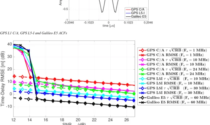
7.2.1 Delay estimation: The main time-delay CRB and CMLE
results for the different signals considered in this study (see Table 1) are summarised in Fig. 4. First, notice that the CMLE asymptotic region threshold (i.e. the operation point where the MLE starts to rapidly deviate from the CRB) is around SNRout= 15 dB. From (22), taking into account that TPRN= 1 ms
for all the signals considered, this threshold corresponds to a
C/N0= 45 dB-Hz using 1 code (TI= 1 ms), C/N0= 39 dB-Hz for
four coherently integrated codes (TI= 4 ms), C/N0= 35 dB-Hz
with ten coherently integrated codes (TI= 10 ms) and C/N0= 32
dB-Hz for the L1 C/A Tbit limit of 20 codes (TI= 20 ms).
Fig. 2 Signals, CRBs, and CMLEs colours and symbols
Table 1 GPS and Galileo signals characteristics. ACF peak
refers to the first zero-crossing of the ACF, TPRN= 1 ms
Signal Modulation Tbit, ms ACF Peak
GPS L1 C/A BPSK(1) 20 ±1.023 μs GPS L5-I BPSK(10) 10 ±0.1023 μs Galileo E5 AltBOC(15,10) 4 ±0.0174 μs
Let us first compare the time-delay estimation results for the GPS L1 C/A signal considering different Fs= 1, 10 and 24 MHz,
the latter being the full signal bandwidth. For a receiver operation point SNRout= 25 dB, which for a nominal C/N0= 45 dB-Hz
corresponds to a standard TI= 10 ms. The time-delay standard
deviation is στ,L1= 6.8 m for Fs= 1 MHz, στ,L1= 2.3 m for Fs= 10 MHz and στ,L1= 1.5 m for Fs= 24 MHz, which justifies
the interest of exploiting the full signal bandwidth. The drawback is that the CMLE convergence to the CRB is slower w.r.t. the
Fs= 1 MHz case (i.e. 15 ≤ SNRout≤ 18 for Fs= 10 MHz and
15 ≤ SNRout≤ 22 for Fs= 24 MHz), but in any case still having a
lower standard deviation w.r.t. lower bandwidths. Second, we can compare these results with larger bandwidth GPS L5 and Galileo E5 signals. Taking as a reference the same receiver operation point SNRout= 25 dB (Fs in MHz), we obtain the following standard
deviations:
• Reference: στ,L1= 1.5 m (Fs= 24 MHz),
• στ,L5= 64 cm (Fs= 10 MHz),
• στ,L5= 39 cm (Fs= 30 MHz),
• στ,E5= 13 cm (Fs= 60 MHz).
These results clearly show the huge time-delay estimation performance improvement that one can achieve using signals with a large bandwidth, and particularly with AltBOC-type signals. For instance, considering the Galileo E5 signal we gain factors 11 and 3 in time-delay standard deviation w.r.t. to the full bandwidth GPS L1 C/A and L5 signals, respectively.
7.2.2 Phase estimation: Notice that the phase CRB in [m] is
obtained as λc/2π CRBφ. We consider first the same value
λc= λL1= 19.03 cm for all signals, to understand the asymptotic
behaviour of the different phase CMLEs. The phase standard deviation for C/N0= 45 dB-Hz and different SNRout= {15, 18, 21, 25, 28} dB are σφ= {3.8, 2.7, 1.9, 1.2, 0.85}
mm, which match the RTK literature where the standard deviation of phase observables is typically in the range of [1–5] mm [58, 59]. It is remarkable that the phase estimation CRB reads CRBφ≃ (1/2SNRout) (i.e. equality for real signals), which implies
that it does not depend on the broadcast signal but on λc and the receiver operation point SNRout, as opposite to the delay
estimation. Therefore using fast codes does not improve the phase estimation w.r.t. the legacy GPS L1 C/A signal. In addition, from (9) we have that the phase CMLE is given by the argument of the cross-ambiguity function evaluated at the delay and Doppler CMLEs. Then, we can expect that if the latter converged to the CRB (i.e. SNRout> threshold, around 15 dB, see Section 7.2.1) the
same applies to the phase estimate, which is confirmed by the CMLE results in Fig. 5. Regardless of λc, all signals share the same
asymptotic behaviour for the phase estimation, which is known to drive the asymptotic RTK performance.
Fig. 3 GPS L1 C/A, GPS L5-I and Galileo E5 ACFs
Fig. 4 Time-delay CRB and CMLE: GPS L1 C/A (Fs= 1, 10, 24 MHz), GPS L5-I (Fs= 10, 30 MHz), and Galileo E5 (Fs= 60 MHz)
Fig. 5 Phase CRB and CMLE with λc= λL1: GPS L1 C/A (Fs= 1, 10, 24 MHz), GPS L5-I (Fs= 10, 30 MHz), and Galileo E5
7.3 SPP and RTK scenario description
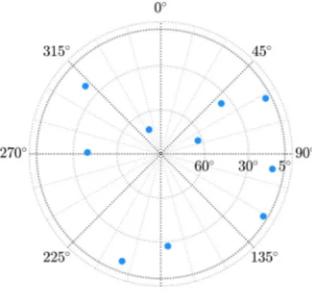
The performance characterisation of SPP and RTK is based on snapshot of simulated GNSS measurements collected at San Fernando (target receiver) and San Roque (base station for RTK) IGS stations on UTC time 04/03/2020 10:00:00. Considering an elevation mask of five degrees, the resulting constellation was depicted in Fig. 6. To segregate the role of geometry and satellite availability across GPS and Galileo from the performance of the studied signals, this work considers the satellites from Fig. 6 as generic, common to GPS and Galileo. Next, the SPP and RTK positioning techniques will be characterised from a two-fold perspective: the estimation of tight lower CRBs and the associated root-mean-square error (RMSE) for the ML estimates for both SPP and RTK positioning methods. The resulting RMSE obtained in the following experiments are, for every signal tested, product of 104
Monte–Carlo runs.
7.4 Case I: SPP performance analysis
Before analysing the GNSS RTK positioning and clearly see which is the ultimate positioning gain with respect to standard GNSS SPP PVT solutions, we analyse the latter considering the problem formulation in Section 3.3. For this purpose, we resort to the CRB derived from (20) with the appropriate matrices D and Cn, i.e. only considering pseudo-ranges and not phase observables. Notice that ionospheric, tropospheric, and instrumental delays are disregarded in the analysis, since it is of our interest to examine the influence of the different signals, integration times and the receiver operation points rather than the model mismatch of the different atmospheric models typically applied. The CRB and CMLE results for the SPP position computation, considering the different signals in Table 1, are shown in Fig. 7. Again, considering a receiver operation point SNRout= 25 dB, we obtain the following positioning RMSE:
• GPS L1 C/A Fs= 1 MHz – RMSE = 10.3 m. • GPS L1 C/A Fs= 10 MHz – RMSE = 3.3 m. • GPS L1 C/A Fs= 24 MHz – RMSE = 2.36 m. • GPS L5 Fs= 10 MHz – RMSE = 1 m. • GPS L5 Fs= 30 MHz – RMSE = 62.5 cm. • Galileo E5 Fs= 60 MHz – RMSE = 18.5 cm.
For code-based PVT solutions, analogously to the time-delay estimation case in Section 7.2.1, it is clear that using large bandwidth signals such as GPS L5 or Galileo E5 has a huge impact on the achievable positioning precision.
7.5 Case II: RTK performance analysis with λc= λL1
As done for the previous SPP case, we want to assess the ultimate achievable performance of RTK positioning techniques and the impact that different GNSS signals may have in such performance. Although it is a common practice for RTK positioning to use multi-constellation/multi-frequency combinations, we are interested in observing the performance gain from every individual GNSS signal. In practice, the characteristics on base and rover receivers may differ, presenting different operation points and/or integration times. For the experimental case at hand, the two receivers are assumed to present the same SNRout and, therefore, the general
stochastic model in (9d) holds valid. First notice that the RTK float solution (i.e. related to the corresponding CRBreal) refers to the real
estimation part in (11a), i.e. disregarding the integer nature of ambiguities. The RTK estimation process follows the three-step decomposition described in (11), where the ILS is resolved based on the LAMBDA method with shrinking search [60]. The RTK fixed solution (i.e. related to the corresponding CRBreal/integer)
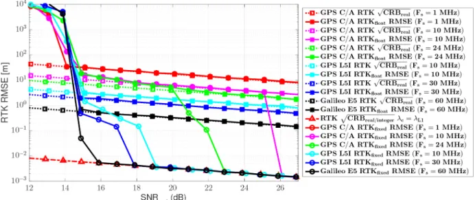
refers to the estimate of the mixed real-ILS in (11c), regardless of whether the ILS correctly computes the correct ambiguities. The position RMSE results are summarised in Fig. 8. We can draw the following conclusions:
(i) Notice that the RTKfixed solution using the GPS L1 C/A signal
with Fs= 1 MHz is the same as the RTKfloat solution, i.e. the ILS
does not correctly fix the ambiguities and therefore the solution obtained is exploring all the ambiguities around the maximum of the code ACF. Notice that higher SNRout values for the GPS L1
C/A signal could be considered, which would involve extending the integration time either coherently or non-coherently. The current configuration with an integration of Tbit= 20 ms, which is the coherent integration limit, is not useful for RTK positioning. (ii) From the previous point, it is clear that if RTK has to be implemented using GPS L1 C/A signals, a higher bandwidth must be considered. For instance, the convergence of the RTKfixed to the corresponding CRBreal/integer, using a GPS L1 C/A signal with Fs= 10 MHz, is given by SNRout= 26 dB, which for the maximum
coherent integration time TI= 20 ms corresponds to a C/N0= 43
dB-Hz, which is a nominal value in clear sky conditions. Therefore, a bandwidth around 10 MHz can be taken as a minimum for GPS L1 C/A-based RTK positioning under nominal propagation conditions (i.e. this value matches standard GNSS receiver architectures which typically operate in Fs∈ [8 − 12]
MHz).
(iii) For any GNSS signal, there exists a threshold receiver operation point for which the RTKfixed rapidly converges to the
RTKfloat solution. Indeed, once a certain noise level threshold is
exceeded (i.e. a delay/phase estimation precision), the use of ILS to fix the ambiguities is not needed. Remarkably, this threshold does not depend on the phase estimation precision but on the code-based delay estimation precision. This is clear in Fig. 8 where we can see that using the Galileo E5 signal we gain {10, 7, 3, 2} dB on the SNRout receiver operation threshold point w.r.t. the GPS L1 C/A Fs= 10 MHz, GPS L1 C/A Fs= 24 MHz, GPS L5-I Fs= 10 MHz
and GPS L5-I Fs= 30 MHz, respectively. Therefore, this clearly justifies the use of fast codes (i.e. both E5 and L5 signals) to provide an improved operation range of RTK architectures.
Fig. 6 Sky plot for the experimentation
Fig. 7 SPP position CRB (dashed lines) and associated RMSE (solid lines)
versus SNR for GPS L1 C/A (Fs= 1, 10, 24 MHz), GPS L5-I
(iv) The SNRout= 16 dB RTK threshold for the Galileo E5 signal
suggests the validity of this RTK solution in a wide range of applications, i.e. in near-indoor weak signal environments.
(v) To summarise, if a new GNSS signal was designed for precise positioning, the recommendation is to use a carrier frequency as high as possible and a signal modulation with the largest signal bandwidth, the former driving the asymptotic RTK performance and the latter the threshold region.
To complete the discussion, we show that considering the corresponding λc for the different signals does not change the asymptotic behaviour, therefore these conclusions are valid irrespective of the considered signal.
7.6 Case III: RTK performance with λL1, λL5, and λE5
7.6.1 Phase estimation: In practice, we have different
wavelengths for each signal: λL1= 19.03 cm, λL5= 25.48 cm, and λE5= 25.15 cm. In this case, the phase standard deviations are
summarised in Table 2, and the corresponding phase RMSE is given in Fig. 9. The slightly different carrier wavelength induce a slight performance loss using lower frequencies, w.r.t. GPS C/A L1, which uses the higher frequency. This will in turn have an impact on the final RTK performance.
7.6.2 RTK performance: As expected, a slight difference in the
phase estimation performance has a slight impact on the RTK solution, but what is remarkable is that this does not change the asymptotic estimation behaviour. The results for different λc are summarised in Fig. 10. Notice that we preserve the same SNR threshold regions as in Fig. 8, and the same convergence to the RTKfloat solutions, therefore, the previous conclusions are valid
whatever the signal carrier frequency.
8 Conclusions
The main goal of this contribution was to characterise the SPP and RTK estimation performance from the baseband signals, i.e. from time-delay and phase estimation, to the final position estimate. Indeed, the input to the standard ML-type positioning solution is the variance of the so-called pseudo-range and phase observables which is in turn determined by the corresponding time-delay and phase estimation precision. In that perspective, a new compact CRB was derived for the joint time-delay, Doppler, phase and amplitude estimation for the narrowband signal model. This CRB is a particular case of a new compact CRB for the generic CSM also provided in this study. A particularly interesting feature is that this new CRB was expressed in terms of the signal samples, making it especially easy to use irrespective of the considered baseband signal. In addition, joint time-delay, Doppler, phase and amplitude estimation using narrowband signals is encountered in a
Fig. 8 RTK position CRBs and RMSE with the same λc= λL1, for GPS L1 C/A (Fs= 1, 10, 24 MHz), GPS L5-I (Fs= 10, 30 MHz), and Galileo E5
(Fs= 60 MHz)
Table 2 Phase estimation standard deviation [mm] for
different λc. SNRout in [dB], coherent integration time TI in [ms]
and C/N0= 45 [dB-Hz] SNRout, dB TI, ms λL1, σφ, mm λL5, σφ, mm λE5, σφ, mm 15 1 3.8 5.1 5.0 18 2 2.7 3.6 3.6 21 4 1.9 2.6 2.5 25 10 1.2 1.6 1.6 28 20 0.85 1.1 1.1
Fig. 9 Phase CRB and CMLE with the corresponding λL1, λL5, and λE5: GPS L1 C/A (Fs= 1, 10, 24 MHz), GPS L5-I (Fs= 10, 30 MHz), and
Galileo E5 (Fs= 60 MHz)
multitude of applications, therefore this tractable CRB constitutes a key tool of broad interest.
Considering the legacy GPS L1 C/A signal as a benchmark and fast codes such as GPS L5 and Galileo E5 signals, it was shown the impact that the GNSS signal has in the different receiver operation steps, and the achievable estimation performance for (i) time-delay estimation, (ii) phase estimation, (iii) SPP position estimation, and (iv) RTK position estimation. A fundamental point with any maximum likelihood estimation procedure is the determination of the threshold region, i.e. the SNR value at the output of the matched filter for which the estimator completely deviates from the CRB. It was found that irrespective of the signal considered, the SNR threshold for both time-delay and phase estimation is around 15 dB. This was also the case for the SPP code-based position estimation, for which it was shown that using a Galileo E5 signal can provide a huge performance gain, potentially reaching standard deviations below 20 cm.
For RTK positioning, the new CRB and the proposed analysis provided even more interesting results. In fact, it was shown that the SNR threshold region is driven by the time-delay precision and not the phase one. Using fast codes, we may have up to 10 dB of gain in the threshold, which in turn implies the validity of such RTK solutions in a wider range of applications. Also, notice that this threshold can be used to determine for which operation regions it is worth to exploit phase measurements, because above the threshold the RTK fixed solution rapidly converges to the float (i.e. real) one. These results hold whatever the signal carrier frequency. To summarise, if a new GNSS signal was to be designed for precise positioning, the recommendation would be to use a carrier frequency as high as possible and a signal modulation with the largest signal bandwidth, the former driving the asymptotic RTK performance, and the latter the threshold region.
9 Acknowledgments
This research was partially supported by the DGA/AID projects (2019.65.0068.00.470.75.01, 2018.60.0072.00.470.75.01), the TéSA Lab Postdoctoral Research Fellowship, and the National Science Foundation under Awards CNS-1815349 and ECCS-1845833.
10 References
[1] Van Trees, H.L.: ‘Detection, estimation, and modulation theory, part III: radar – sonar signal processing and Gaussian signals in noise’ (John Wiley & Sons, USA, 2001)
[2] Chen, J., Huang, Y., Benesty, J.: ‘Time delay estimation’, in Huang, Y., Benesty, J. (eds.): ‘Audio signal processing for next-generation multimedia communication systems’ (Springer, Boston, MA, USA, 2004), pp. 197–227 [3] Levy, B.C.: ‘Principles of signal detection and parameter estimation’
(Springer, Netherlands, 2008)
[4] Mengali, U., D'Andrea, A.N.: ‘Synchronization techniques for digital receivers’ (Plenum Press, New York, USA, 1997)
[5] Fernández-Prades, C., Lo Presti, L., Falletti, E.: ‘Satellite radiolocalization from GPS to GNSS and beyond: novel technologies and applications for civil mass market’, Proc. IEEE, 2011, 99, (11), pp. 1882–1904
[6] Amin, M.G., Closas, P., Broumandan, A., et al.: ‘Vulnerabilities, threats, and authentication in satellite-based navigation systems [scanning the issue]’, Proc. IEEE, 2016, 104, (6), pp. 1169–1173
[7] Yan, J., Tiberius, C.C.J.M., Janssen, G.J.M., et al.: ‘Review of range-based positioning algorithms’, IEEE Trans. Aerosp. Electron. Syst., 2013, 28, (8), pp. 2–27
[8] Zavorotny, V.U., Gleason, S., Cardellach, E., et al.: ‘Tutorial on remote sensing using GNSS bistatic radar of opportunity’, IEEE Geosci. Remote Sens. Mag., 2014, 2, (4), pp. 8–45
[9] Lestarquit, L., Peyrezabes, M., Darrozes, J., et al.: ‘Reflectometry with an open-source software GNSS receiver: use case with carrier phase altimetry’, IEEE J. Sel. Top. Appl. Earth Obs. Remote Sens., 2016, 9, (10), pp. 4843– 4853
[10] Cardellach, E., Li, W., Rius, A., et al.: ‘First precise spaceborne sea surface altimetry with GNSS reflected signals’, IEEE J. Sel. Top. Appl. Earth. Obs. Remote Sens., 2019, 13, pp. 102–112
[11] Schreier, P.J., Scharf, L.L.: ‘Statistical signal processing of complex-valued data’ (Cambridge University Press, UK, 2010)
[12] Schweppe, F.C.: ‘Sensor array data processing for multiple signal sources’, IEEE Trans. Inf. Theory, 1968, 14, pp. 294–305
[13] Stoica, P., Nehorai, A.: ‘Performances study of conditional and unconditional direction of arrival estimation’, IEEE Trans. Acoust. Speech, Signal Process., 1990, 38, (10), pp. 1783–1795
[14] Scharf, L.L.: ‘Statistical signal processing: detection, estimation, and time series analysis’ (Addison-Wesley, USA, 2002)
[15] Van Trees, H.L.: ‘Optimum array processing’ (Wiley-Interscience, New-York, 2002)
[16] Renaux, A., Forster, P., Chaumette, E., et al.: ‘On the high-SNR conditional maximum-likelihood estimator full statistical characterization’, IEEE Trans. Signal Process., 2006, 54, (12), pp. 4840–4843
[17] Ottersten, B., Viberg, M., Stoica, P., et al.: ‘Exact and large sample maximum likelihood techniques for parameter estimation and detection in array processing’, in Haykin, S., Litva, J., Shepherd, T.J. (eds.): ‘Radar array processing’ (Springer-Verlag, Heidelberg, 1993), pp. 99–151
[18] Tsao, J., Steinberg, B.D.: ‘Reduction of sidelobe and speckle artifacts in microwave imaging: the CLEAN technique’, IEEE Trans. Antennas Propag., 1988, 36, (4), pp. 543–556
[19] Ziskind, I., Wax, M.: ‘Maximum likelihood localization of multiple sources by alternating projection’, IEEE Trans. Acoust. Speech Signal Process., 1988,
36, (10), pp. 1553–1560
[20] Stoica, P., Söderström, T.: ‘On reparametrization of loss functions used in estimation and the invariance principle’, Signal Process., 1989, 17, pp. 383– 387
[21] Antreich, F., Nossek, J.A., Seco-Granados, G., et al.: ‘The extended invariance principle for signal parameter estimation in an unknown spatial field’, IEEE Trans. Signal Process., 2011, 59, (7), pp. 3213–3225
[22] Swindlehurst, A.L., Stoica, P.: ‘Maximum likelihood methods in radar array signal processing’, Proc. IEEE, 1998, 86, (2), pp. 421–441
[23] Vincent, F., Chaumette, E., Charbonnieras, C., et al.: ‘Asymptotically efficient GNSS trilateration’, Signal Process., 2017, 133, pp. 270–277
[24] Closas, P., Fernández-Prades, C., Fernández-Rubio, J.A.: ‘Maximum likelihood estimation of position in gnss’, IEEE Signal Process. Lett., 2007,
14, (5), pp. 359–362
[25] Closas, P., Gusi-Amigó, A.: ‘Direct position estimation of GNSS receivers: analyzing main results, architectures, enhancements, and challenges’, IEEE Signal Process. Mag., 2017, 34, (5), pp. 72–84
[26] Eueler, H.J., Goad, C.C.: ‘On optimal filtering of gps dual frequency observations without using orbit information’, Bull. Géodésique, 1991, 65, (2), pp. 130–143
[27] Kuusniemi, H., Wieser, A., Lachapelle, G., et al.: ‘User-level reliability monitoring in urban personal satellite-navigation’, IEEE Trans. Aerosp. Electron. Syst., 2007, 43, (4), pp. 1305–1318
[28] Medina, D., Gibson, K., Ziebold, R., et al.: ‘Determination of pseudorange error models and multipath characterization under signal-degraded scenarios’. Proc. 31st Int. Technical Meeting of the Satellite Division of The Institute of Navigation (ION GNSS + 2018), Miama, FL, USA, 2018, pp. 24–28 [29] Dogandzic, A., Nehorai, A.: ‘Cramér-rao bounds for estimating range,
velocity, and direction with an active array’, IEEE Trans. Signal Process., 2001, 49, (6), pp. 1122–1137
[30] Noels, N., Wymeersch, H., Steendam, H., et al.: ‘True cramér-rao bound for timing recovery from a bandlimited linearly modulated waveform with unknown carrier phase and frequency’, IEEE Trans. Commun., 2004, 52, (3), pp. 473–483
[31] Closas, P., Fernández-Prades, C., Fernández-Rubio, J.A.: ‘Cramér-rao bound analysis of positioning approaches in GNSS receivers’, IEEE Trans. Signal Process., 2009, 57, (10), pp. 3775–3786
[32] Enneking, C., Steint, M., Castaneda, M., et al.: ‘Multi-satellite time-delay estimation for reliable high-resolution GNSS receivers’. Proc. IEEE/ION PLANS, Myrtle Beach, SC, USA, 2012
[33] Chen, Y., Blum, R.S.: ‘On the impact of unknown signals on delay, Doppler, amplitude, and phase parameter estimation’, IEEE Trans. Signal Process., 2019, 67, (2), pp. 431–443
[34] Bartov, A., Messer, H.: ‘Lower bound on the achievable DSP performance for localizing step-like continuous signals in noise’, IEEE Trans. Signal Process., 1998, 46, (8), pp. 2195–2201
[35] Kay, S.M.: ‘Fundamentals of statistical signal processing: estimation theory’ (Prentice-Hall, Englewood Cliffs, New Jersey, USA, 1993)
[36] Yau, S.F., Bresler, Y.: ‘A compact Cramér-Rao bound expression for parametric estimation of superimposed signals’, IEEE Trans. Signal Process., 1992, 40, (5), pp. 1226–1230
[37] Williams, N., Wu, G., Closas, P.: ‘Impact of positioning uncertainty on eco approach and departure of connected and automated vehicles’. 2018 IEEE/ION Position, Location and Navigation Symp. (PLANS), Monterey, CA, USA, 2018, pp. 1081–1087
[38] Teunissen, P.J.G., Montenbruck, O. (Eds.): ‘Handbook of global navigation satellite systems’ (Springer, Switzerland, 2017)
[39] Rife, D.C., Boorstyn, R.R.: ‘Single tone parameter estimation from discrete-time observations’, IEEE Trans. Inf. Theory, 1974, 20, (5), pp. 591–598 [40] D'Andrea, A.N., Mengali, U., Reggiannini, R.: ‘The modified Cramér–Rao
bound and its application to synchronization problems’, IEEE Trans. Commun., 1994, 42, (2/3/4), pp. 1391–1399
[41] Smith, S.T.: ‘Statistical résolution limits and the complexified Cramér–Rao bound’, IEEE Trans. Signal Process., 2005, 53, (5), pp. 1597–1609 [42] El Korso, M.N., Boyer, R., Renaux, A., et al.: ‘Conditional and unconditional
cramér-rao bounds for near-field source localization’, IEEE Trans. Signal Process., 2010, 58, (5), pp. 2901–2907
[43] Wu, N., Wang, H., Zhao, H., et al.: ‘Evaluation of cramér-rao bounds for phase estimation of coded linearly modulated signals’. Proc. IEEE Vehicular Technology Conf., Vancouver, BC, Canada, 2014
[44] Steendam, H., Moeneclaey, M.: ‘Low-SNR limit of the cramér-rao bound for estimating the time-delay of a PSK, QAM, or PAM waveform’, IEEE Commun. Lett., 2001, 5, (1), pp. 31–33
[45] Van Trees, H.L., Bell, K.L., Tian, Z.: ‘Detection, estimation and modulation theory – part 1’ (Wiley, USA, 2013, 2nd edn.)
[46] Wang, P., Orlik, P.V., Sadamoto, K., et al.: ‘Cramér–rao bounds for a coupled mixture of polynomial phase and sinusoidal FM signals’, IEEE Signal Process Lett., 2017, 24, (6), pp. 746–750