Astronomy& Astrophysics manuscript no. aa ©ESO 2021 March 8, 2021
Convective core sizes in rotating massive stars
I. Constraints from solar metallicity OB field stars
S. Martinet
1, G. Meynet
1, S. Ekström
1, S. Simón-Díaz
2, 3, G.Holgado
4, N. Castro
5, C. Georgy
1, P. Eggenberger
1, G.
Buldgen
1, S. Salmon
1, R. Hirschi
6, 7, J. Groh
8, E. Farrell
8, and L. Murphy
81 Department of astronomy, University of Geneva, chemin Pegasi 51, 1290 Versoix, Switzerland
e-mail: [email protected]
2 Instituto de Astrofísica de Canarias, Avenida Vía Láctea, E-38205 La Laguna, Tenerife, Spain
3 Universidad de La Laguna, Dpto. Astrofísica, E-38206 La Laguna, Tenerife, Spain
4 Centro de Astrobiología, ESAC campus, Villanueva de la Cañada, E-28 692, Spain
5 Leibniz-Institut für Astrophysik Potsdam, An der Sternwarte 16, 14482 Potsdam, Germany
6 Astrophysics group, Keele University, Keele, Staffordshire ST5 5BG, UK
7 Institute for the Physics and Mathematics of the Universe (WPI), University of Tokyo, 5-1-5 Kashiwanoha, Kashiwa 277-8583,
Japan
8 Trinity College Dublin, The University of Dublin, Dublin, Ireland
March 8, 2021
ABSTRACT
Context. Spectroscopic studies of Galactic O and B stars show that many stars with masses above 8 M have been observed in
the Hertzsprung-Russell (HR) diagram just beyond the main-sequence (MS) band, as predicted by stellar models computed with a moderate overshooting. This may be an indication that the convective core sizes in stars in the upper part of the HR diagram are larger than predicted by these models.
Aims.Combining stellar evolution models and spectroscopic parameters derived for a large sample of Galactic O and B stars with the inclusion of brand-new information about their projected rotational velocities, we reexamine the question of the convective core size in MS massive stars.
Methods.We computed a grid of 120 different stellar evolutionary tracks with three initial rotations at solar metallicity (Z = 0.014),
spanning a mass range from 7 to 25 M , and combining different values for the initial rotation rate and overshooting parameter. For
the rotating models, we considered two cases, one with a moderate and one with a strong angular momentum transport, the latter imposing a solid body rotation during most of the MS phase. We confront the results with two observed features: the position of the terminal age main sequence (TAMS) in the HR diagram and the decrease of the surface rotation when the surface gravity decreases at the end of the MS phase.
Results.We confirm that for stars more massive than about 8 M , the convective core size at the end of the MS phase increases
more rapidly with the mass than in models computed with a constant step overshoot chosen to reproduce the main sequence width
in the low mass range (around 2 M ). This conclusion is valid for both the cases of non-rotating models and rotating models either
with a moderate or a strong angular momentum transport. The increase of the convective core mass with the mass obtained from the
TAMS position is, however, larger than the one deduced from the surface velocity drop for masses above about 15 M . Although the
observations that are available at present cannot determine the best choice between the core sizes given by the TAMS and the velocity drop, we discuss various methods of escaping this dilemma. At the moment, comparisons with eclipsing binaries seem to favor the solution given by the velocity drop.
Conclusions.While we confirm the need for larger convective cores at higher masses, we find tensions among different methods for
stars more massive than 15 M . The use of single-aged stellar populations (non-interacting binaries or stellar clusters) would be a
great asset in resolving this tension.
Key words. stars: evolution – stars: rotation – stars: massive – stars: fundamental parameters – stars: interiors – stars: statistics
1. Introduction
The size of convective cores is an long-standing problem that was investigated very early on by, among others, Saslaw & Schwarzschild (1965), Shaviv & Salpeter (1973), Maeder (1975), Roxburgh (1978), and Bressan et al. (1981), as well as further on by Renzini (1987), Maeder & Meynet (1987a), and Zahn (1991). The convective boundaries are defined in stellar models by the Schwarzschild or Ledoux criterion. Both criteria give the position inside the star where the acceleration resulting from the net balance between the gravity and the buoyancy force
becomes zero (Maeder & Stahler 2009). However, it neglects the inertia of the convective elements, which will pursue their move-ments beyond the limit where the acceleration is zero up to the point where the velocity is zero. While the physics of this process is very basic, there are many different ways to implement it in stellar models (see Gabriel et al. 2014). The two most frequently used methods at the moment are known as “step overshoot” as applied, for example, in Ekström et al. (2012) when defining an overshooting parameter, αov, extending the convective radius
in-stantaneously by a fraction of the pressure scale height; whereas “diffusive overshoot’, for example, as implemented in Herwig
et al. (1997), Paxton et al. (2011), Choi et al. (2016), proposes an overshooting parameter, fov, intervening in a depth-dependent
diffusion coefficient.
The overshooting process is not the only physical process impacting the size of the convective cores. Effects such as rota-tion, tides, or even the presence of an internal magnetic field can all affect the sizes of the convective cores. This complicates the issue and makes it difficult to find a solution.
In recent decades, various attempts have been made to con-strain the size of the convective core using well-observed fea-tures: the main-sequence (MS) band width in the Hertzsprung-Russell (HR) diagram (Maeder & Mermilliod 1981, Barbaro & Pigatto 1984, Castro et al. 2014), the drop of the surface rotation velocity when plotted as a function of the surface gravity (Brott et al. 2011), or even the extension of the blue loops during the core He-burning phase (Matraka et al. 1982, Miller et al. 2020). Castro et al. (2014) presented, for the first time, the distribu-tion of a large sample of Galactic massive stars in the spectro-scopic HR diagram (based on the gravity-effective temperature diagram, see Langer & Kudritzki 2014), and showed that stel-lar models from Ekström et al. (2012) exhibit a good agreement with the MS width for stars around 8 M , while a better
agree-ment for stars around 15 M was found for the models from Brott
et al. (2011) with larger convective core sizes. This led to suggest a possible scaling of the overshooting with mass. Claret & Torres (2016, 2017, 2018, 2019) also provided empirical evidence from the study of a sample of eclipsing binaries that there is a clear and steep increase of the overshooting from 1.2 to 2 M , and
that it remains constant thereafter out to at least 4.4 M . Recently
Higgins & Vink (2019), Tkachenko et al. (2020) used eclipsing binaries to constrain stellar models. Using non-rotating stellar models, Tkachenko et al. (2020) find convective core masses tween 17 and 35% of the stellar mass for stars with masses be-tween 5 and 16 M 1.
A drop of the surface velocity is expected to occur just after the MS phase when the star rapidly crosses the HR gap and be-comes first a blue and then a red supergiant. By studying a sam-ple of about 400 O- and B-type stars in the Magellanic Clouds, Hunter et al. (2008) observed a steep drop in the distribution of projected rotational velocities as a function of surface gravity (g) at log(g) ∼3.2 and suggested the slower B supergiants could be post-MS stars. Brott et al. (2011) used this steep drop to con-strain the core overshooting parameter in massive star models, while Vink et al. (2010) proposed another interpretation of this drop as being due to an increase of the mass loss connected with the effect of the so-called bi-stability jump at Teff= 22000 K.
Additional constraints are available from asteroseismology studies (Appourchaux et al. 2015). For low-mass stars (below 1.6 M ), Deheuvels et al. (2016) find hints of overshooting
scal-ing with mass. Usscal-ing the stellar evolution code CESAM2K, im-plementing a step overshoot, they obtain values for the exten-sion of the convective core size that are similar to the values obtained by Ekström et al. (2012) for the non-rotating models. Bossini et al. (2017) revealed the need for a moderate overshoot-ing while studyovershoot-ing red clump stars in field and open clusters. In-version techniques (Roxburgh & Vorontsov 2002, Buldgen et al. 2018) are also used to obtain additional constraints. Slowly pul-sating main-sequence B stars between 2.5 and 8 M , δ Scuti/ γ
Dor hybrid stars have also been studied to derive the extension of the core (Moravveji et al. 2015, 2016, Szewczuk & Daszy´nska-Daszkiewicz 2018, Murphy et al. 2016). More massive stars, β
1 In Sect. 5, we compare these convective core mass fractions with
those obtained in the present work.
Cephei stars (typically between 6-8 and 20 M ) have been
stud-ied by, among others, Aerts et al. (2003), Dupret et al. (2004), Handler et al. (2005), Mazumdar et al. (2006), Briquet et al. (2007), and have been reviewed by Aerts (2015).
The range of convective core sizes deduced from these dif-ferent studies is still large, which may be understood due to the fact that, as mentioned above, many factors, which may differ from star to star, have an impact as the initial mass, the age, the chemical composition, the rotation, and even on the mass trans-fer history (see Klencki et al. 2020). Moreover, asteroseismolog-ical features, as well as the observation of the MS band, cannot specifically constrain the physical process determining the con-vective core size. To do so, we should identify a feature that only depends on this specific process.
Another approach is to use sophisticated 3D hydrodynamical simulations. These simulations can guide the building of new prescriptions for determining the sizes of the convective regions in 1D stellar evolution codes2. For instance, simulations such
as those of Meakin & Arnett (2007) and Cristini et al. (2019) have shown that the upper boundary of a convective zone may evolve in a way that is not predicted by present 1D stellar models through a process called the mixing boundary entrainment. Some first tests are underway, implementing these new prescriptions in 1D stellar models (Scott et al. submitted).
In the present work, we follow a more classical approach consisting of calibrating the size of the convective cores using observed features dependent on it, as done in previous works (see e.g., Brott et al. 2011, Ekström et al. 2012). However, at the moment, very few authors (if any) have considered the use of more than one observed feature when performing such calibra-tions. This actually may provide a biased view in the sense that confronting the models with only one observational constraint does not guarantee that the others will be fitted too. The present work is an attempt to perform comparisons with two observed features 3: (1) the position of the terminal age main sequence
(TAMS) line in the HR diagram; (2) the position of the drop of the surface velocity in the υ sin i versus surface gravity diagram. For the above comparisons, we use two types of rotating models. One set of models uses a given physic input exactly similar to the one used in our grids of models (Ekström et al. 2012), where during the MS phase, some differential rotation between the core and the envelope develops (moderate angular momentum transport). A second set has been obtained assum-ing that stars rotate as solid bodies durassum-ing most of the MS phase (strong angular momentum transport). This allows us to investi-gate, within the framework of a given stellar evolution code, the dependence of the size of the convective core on the angular and chemical mixing processes.
The paper is organized as follows. The physical ingredients of the models are discussed in Sect. 2. The properties of the models and the impact of overshooting are discussed in Sect. 3, while comparisons with massive stars observations is carried out in Sect. 4. We discuss some limitations of the present approach in Sect. 5. We describe our main findings in Sect. 6.
2 Three-dimensional stellar models are too computationally expensive
for allowing to follow the evolution of the limit of the convective core during even a significant fraction of the MS phase.
3 Other observed features such as the extension of the blue loops and
the chemical enrichment of the stellar surface during the evolution of massive stars could also be incorporated to such investigation (see Sect. 6).
2. Physical ingredients and models computed
A detailed description of the physics included in the models can be found in Ekström et al. (2012). Here, we briefly describe two aspects that are relevant for the present work: overshooting and rotation.
2.1. Overshooting
In the stellar grids published thus far (Ekström et al. 2012, Georgy et al. 2013, 2014b), we used models computed with the Schwarzschild criterion and a step overshooting. In these mod-els, the radius of the convective core is obtained in the following way:
Rconv= Rconv-Sch+ α × Hp, (1)
where Rconv-Sch is the radius given by the Schwarzschild
criterion, Hp is the pressure scale height estimated at the
Schwarzschild radius, and α is a free parameter. In all these mod-els, a value of α = 0.1 was chosen in order to fit the empirical width of the MS obtained for solar metallicity stars with initial masses in the 1.7 – 2.5 M range. This value is kept constant for
all the initial masses above 1.7 M , for the different metallicities
and for core H- and He-burning phases.
The implementation, shown in Eq. 1, is very simple. How-ever, here we should recall three points. First, in the whole con-vective core (i.e., the Schwarzschild core plus the overshoot-ing region), the temperature gradient is the adiabatic one. Sec-ond, the chemical species are completely homogenized in the whole core at every time step during the core H and He-burning phases.4Finally, we do not consider any overshooting at the bor-ders of the intermediate convective shells or at the bottom of the convective envelope. A brief discussion of these limitations is provided in Sect. 5.
It is also important to remember that while penetrative and diffusive overshooting are quite different, the physical properties at the border of the core are quite similar among non-rotating diffusive models and our penetrative rotating models, even for slow rotators (see Miglio et al. 2009, Salmon 2014). A more in-depth discussion can be found in Sect. 5.
2.2. Rotation
The way the rotation physic is included in the Geneva stellar evo-lution code (GENEC) is presented in Eggenberger et al. (2008, also see references therein). In the case of models with a moder-ate angular momentum transport, we use the same prescriptions as in Ekström et al. (2012). In particular, we use the shear dif-fusion coefficient as given by Maeder (1997) and the horizontal diffusion coefficient from Zahn (1992). An advective equation is solved for describing the transport of the angular momentum by the meridional currents during the MS phase.
We also considered the case of a very efficient angular mo-mentum transport to take into account the need for a more effi-cient transport process in asteroseismologic studies of subgiants and giants (Deheuvels et al. 2012, Deheuvels et al. 2015, Mosser et al. 2012, den Hartogh et al. 2019). For this, we used a diffusive approach for the angular momentum transport by the meridional
4 In the more advanced phases of the evolution, when the nuclear
burn-ing time of some elements in some deep layers of the convective core becomes shorter than the timescale for the mixing in that core, the
com-plete homogenization is no longer realized. A diffusive approach has
then to be used for mixing the elements in the convective regions.
currents, with a very large diffusive coefficient as given by Song et al. (2016). Due to the nearly constantΩ profile, transport of chemical elements by shear mixing is negligible. On the other hand, their transport by meridional currents is very strong. These models, for a given initial mass, rotation, and at a given age, are much more mixed than the models with a moderate angular mo-mentum transport.
2.3. Models computed
The grid is composed of 120 different stellar evolutionary tracks at Z = 0.014, with initial masses equal to 7, 9, 15, and 25 M ,
with six different overshooting parameters ranging from 0.1 to 0.6, with surface rotation at the equator (υ) on the ZAMS equal to 0, 0.2, and 0.4 the critical velocity5(υ
crit). Each rotating model
is computed with a moderate and a strong angular momentum transport. All the models were computed until at least the maxi-mum redward extension of the track in the HRD during the core H-burning phase ( i.e. TAMS). Actually, except in a few cases (exactly 17 models), all models were computed until the end of the core H-burning phases. Those that were stopped before this point are chemically mixed to a significant extent and do not con-tribute to the extension of the MS band width beyond its exten-sion obtained from slower or non-rotating models. A little more than one-third of the models (42 exactly) were also computed over the whole core He-burning phase.
3. Impact of overshooting and rotation
3.1. Hertzsprung-Russell diagram
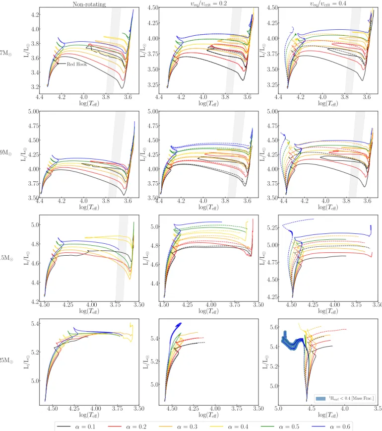
Figure 1 presents the evolutionary tracks for the different initial mass models considered in this work, non-rotating and rotating, with various overshoots. Let us call the "red hook" the point on the MS band where the tracks reach their lowest effective tem-perature before turning back, for a short time, to bluer regions of the HR diagram. As the overshooting parameter increases, the red hook occurs in general at a higher luminosity and a lower effective temperature. There are exceptions to this general trend occurring for the most chemically mixed models (see, e.g., the models computed with υ/υcrit = 0.4 and a strong angular
mo-mentum transport shown by the dashed lines in the right panels of Fig. 1).
The blue tracks for the 25 M in the lower right panel
(υ/υcrit = 0.4, both with a moderate and a strong angular
mo-mentum transport and an overshooting parameter equal to 0.6), actually show surface abundances during the MS phase that are similar to the surface abundances observed at the surface of Wolf-Rayet stars. Due to our prescriptions for computing the mass-loss rates, much stronger stellar winds appear from that point on and this produces the peculiar shape of the tracks in the regions indicated by the blue shade in the bottom right panel of Fig. 1.
We can also see the differences in the evolutionary tracks when a moderate and a strong angular momentum transport is considered for a given initial mass, rotation, and overshoot. For the velocities υ/υcrit = 0.2, differences are very small. They are
much more important for the cases υ/υcrit = 0.4. A strong
cou-pling implies much more chemically mixed models. This shifts
5 The critical velocity is the value of the equatorial velocity such that
the centrifugal force balances the gravity. The critical velocity in the
frame of the Roche approximation is given by q2
3 GM
Rp,crit, where Rp,critis
3.6 3.8 4.0 4.2 4.4 log(Teff) 3.2 3.4 3.6 3.8 4.0 4.2 L/L Red Hook Non-rotating 3.6 3.8 4.0 4.2 4.4 log(Teff) 3.25 3.50 3.75 4.00 4.25 4.50 L/L υeq/υcrit= 0.2 3.6 3.8 4.0 4.2 4.4 log(Teff) 3.25 3.50 3.75 4.00 4.25 4.50 L/L υeq/υcrit= 0.4 3.6 3.8 4.0 4.2 4.4 log(Teff) 3.50 3.75 4.00 4.25 4.50 4.75 5.00 L/L 3.6 3.8 4.0 4.2 4.4 log(Teff) 3.50 3.75 4.00 4.25 4.50 4.75 5.00 L/L 3.6 3.8 4.0 4.2 4.4 log(Teff) 3.50 3.75 4.00 4.25 4.50 4.75 5.00 L/L 3.50 3.75 4.00 4.25 4.50 log(Teff) 4.2 4.4 4.6 4.8 5.0 L/L 3.50 3.75 4.00 4.25 4.50 log(Teff) 4.4 4.6 4.8 5.0 L/L 3.50 3.75 4.00 4.25 4.50 log(Teff) 4.25 4.50 4.75 5.00 5.25 L/L 3.50 3.75 4.00 4.25 4.50 log(Teff) 5.0 5.2 5.4 L/L 3.50 3.75 4.00 4.25 4.50 log(Teff) 5.0 5.2 5.4 L/L α = 0.1 α = 0.2 α = 0.3 α = 0.4 α = 0.5 α = 0.6 3.5 4.0 4.5 5.0 log(Teff) 5.0 5.2 5.4 5.6 L/L
1Hsurf< 0.4 [Mass Frac.]
25M
15M 9M 7M
Fig. 1. Evolutionary tracks in the Hertzsprung-Russell diagrams. Non-rotating models are shown in the panels in the left column. The plain lines in the panels of the middle and right column are the rotating models with a moderate angular momentum transport. The dashed lines are the models
computed with a strong angular momentum transport. We note that at low rotations (υ/υcrit = 0.2), models with moderate and strong angular
momentum transport may overlap nearly exactly preventing to see the dashed lines (see e.g., the 7 M stellar model). The shaded area shows the
instability strip (determined as in Anderson et al. 2016). The models were computed up to MS turnoff for most stars, the lowest mass stars were expended up to the end of He-burning. In the bottom right panel, the parts of the tracks where the mass fraction of hydrogen at the surface is below 0.4, meaning the star may be considered a Wolf-Rayet, are highlighted by a broad blue band.
the tracks to the blue with respect to the case of moderate angular momentum transport.
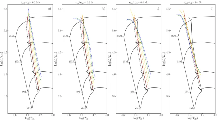
Figure 2 shows how the width of the MS band varies when different values of α are used in different rotating models. We
4.0 4.2 4.4 4.6 log(Teff) 3.5 4.0 4.5 5.0 5.5 log( L/L ) b) 7M 9M 15M 25M υeq/υcrit= 0.2 Sr 4.0 4.2 4.4 4.6 log(Teff) 3.5 4.0 4.5 5.0 5.5 log( L/L ) a) 7M 9M 15M 25M υeq/υcrit= 0.2 Mo 4.0 4.2 4.4 4.6 log(Teff) 3.5 4.0 4.5 5.0 5.5 log( L/L ) c) 7M 9M 15M 25M υeq/υcrit= 0.4 Mo 4.0 4.2 4.4 4.6 log(Teff) 3.5 4.0 4.5 5.0 5.5 log( L/L ) d) 7M 9M 15M 25M υeq/υcrit= 0.4 Sr
Fig. 2. Evolutionary tracks in the HR diagram for non-rotating models with α=0.3 (black solid lines). The limits of the MS band are indicated for various values of α, rotation rates (indicated above each panel), and transport efficiency (see above each panel; Mo/Sr: moderate/strong angular momentum transport). Looking at the bottom of these lines in the left panel, α goes from 0.1 to 0.2, 0.3, 0.4, 0.5, and 0.6, going from left to right.
define the MS band width as the difference, taken at a fixed effective temperature between the luminosity at the red hook and at the ZAMS. Lines connecting the red hooks of models obtained with the same overshooting parameter can be seen in Fig. 2 (dashed lines except for the case α= 0.3 which is shown by a solid line). This width, in general, increases when the over-shooting increases.
For non-rotating models, at higher masses, the position of the red hook in the HRD extends further away to the red than at lower masses. In higher mass models, due to mass losses by stellar winds, the core occupies a larger fraction of the total mass at the end of the MS phase and this shifts the TAMS to the red (see e.g., Maeder & Meynet 1987b).
On the other hand, in the non-rotating models, enlarging the overshoot continuously increases the MS band width (at least in the range of overshoots considered here); for the rotating models, the impacts between 15 and 25 M are very different.
A most striking effect can be seen for the 25 M stellar
mod-els at υ/υcrit= 0.4 with moderate or strong angular momentum.
In those cases, above some overshoot, any further increase of α produces a reduction of the width of the MS band. This can be understood by the fact that rotation has two counteracting effects on the width of the MS band. On one hand, it slows down the decrease in mass of the convective core during the MS phase. On the other hand, rotation also changes the chemical compo-sition in the radiative envelope. Rotation, for instance, makes the radiative envelope more helium-rich. This reduces its opac-ity (massive stars are dominated by electron-scattering opacopac-ity) and makes the track bluer, reducing thus the MS band width. In stars undergoing a strong chemical mixing, this second effect dominates and thus reduces the MS band width compared to ana-log models without rotation. The more massive a star, the more mixed it is (given an initial rotation, whether computed with a
moderate or strong angular momentum transport), thus, this ef-fect appears here only for a mass above a limit between 15 and 25 M . It is interesting to compare panels c and d of Fig. 2. We
see that models with a strong angular momentum transport show less sensitivity on the overshoot than models with a moderate an-gular momentum. This is because models with a strong anan-gular momentum transport are more chemically mixed, making these models less sensitive to larger cores.
3.2. Surface rotation
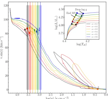
Figure 3 shows the evolution of the surface velocity as a func-tion of the surface gravity for 9 M stellar models computed with
various overshoots and moderate angular momentum transport. After the initial very rapid drop of the surface velocity (see dis-cussion of this feature in Denissenkov et al. 1999, Ekström et al. 2012, Granada & Haemmerlé 2014), the surface rotation varies slowly until the end of the MS phase, which occurs for log(g) between 3.5 and 3.0 in Fig. 3. After the MS phase, we see that the surface velocity drops strongly as the gravity decreases. This is linked to the expansion of the envelope after the end of H-burning. The timescale of the drop is really short compared to the main sequence. Indeed, numbers associated with red squares on Fig. 3 are separated by 105yrs from one another, with square
(2) being the end of the MS, and yet the two first squares are separated by 0.1 dex in log(g), while the next two are separated by more than 3.0 dex in log(g). As noted above, this expansion is rapid and the surface velocity is likely dominated here by the local conservation of the angular momentum. Observationally, Fig. 3 means that very few post-MS stars will be expected in the high-velocity range (near the values at the end of the MS phase), but more will be observed at a much lower gravity when the core-He burning begins.
0.0 0.5 1.0 1.5 2.0 2.5 3.0 3.5 4.0 log(g) [g.cm.s−2] 0 20 40 60 80 100 120 v.sin(i) [km.s − 1] 1 2 3 4.2 4.4 log(Teff) 3.75 4.00 4.25 4.50 log( L/L ) End MS Drop log g α = 0.1 α = 0.2 α = 0.3 α = 0.4 α = 0.5 α = 0.6
Fig. 3. Evolution of the surface velocity as a function of the surface
gravity for 9 M stars rotating at υ/υcrit=0.2 with overshooting scaling
from 0.1 to 0.6, computed with a moderate angular momentum trans-port. The vertical lines show the log(g) maximizing the ratio between the time spent on the left side of the shaded area and the time spent on the right side, computed with Eq. 2. Diamonds show the end of the
MS. Numbers associated with red squares are separated by 105yrs from
one another, with square (2) being the end of the MS. In the upper right corner is the HRD of the same models, with the location of the veloc-ity drop indicated. The drop occurs nearly at the same position as the red hook and thus this feature can be used to observationally detect its position.
We want to have an objective way of determining the log(g)-limit and comparing it among the various models. Since this limit is expected to mark the end of the slow-evolution MS phase and the transition to the rapid HR crossing, we use a considera-tion on the time spent before and after this limit. In Fig. 3, the vertical lines show for each model the log(glim) where the
high-est ratio between the time spent in the shaded area before and after the vertical line is (the black shaded area, for instance, cor-responds to the case of the black track, and the same for the other colors). The position of log (glim) is given by:
log(glim)= Max.
t[log(glim)] − t[log(glim)+ 0.05dex]
t[log(glim) − 0.05] − t[log(glim)]
, (2)
where t[log(glim)] is the age of the star when the surface gravity
is equal to glim.
Here, we used 0.05 dex as the width to search for the max-imizing limit, but lower and higher values have been tested and lead to the same results. Moreover, to exclude the possibility of finding a maximum ratio between two negligible times (com-pared to MS lifetime), we are searching for limits that maximize both the ratio and the total accumulated time. These limits show that indeed the drop in surface velocity occurs at the same po-sition as the red hook and thus can be used to determine the position of this feature.
When increasing the overshooting, the limit shifts to lower log(g). Typically, passing from an overshooting α = 0.1 to 0.3, shifts the value of log(glim) by 0.2 dex towards lower values.
This is larger than the error in log(g) determinations from spec-troscopy (about 0.1 dex). Mass also plays a role in the impact of
overshooting on the log(g) limit as Fig 7 shows. We shall discuss this point in Sect. 4.
4. Comparison with observations
4.1. Width of the main sequence band
Ideally, in order to establish the MS band’s width, well-populated young clusters should be used since they provide the distribution of stars with a unique age and chemical composition. The fact that stars of the same age are observed makes that short phases of the evolution can be populated only by a very small range of initial masses. This is in contrast to the case of a mixed population of stars from different regions of the Galaxy (includ-ing, e.g., clusters of different ages and stars from the field), where the effect of different types of observational biases on the com-piled sample blur the exact location of the end of the MS. In brief, the interpretation of such a survey is more complex than single-aged stellar populations in stellar clusters.
The stellar clusters present, however, their own difficulties. First, there are not so many very populated and well-observed stellar clusters at solar metallicity with turn-off masses in the range of interest here. Second, careful studies aimed at discriminating stars belonging to the clusters from the field stars need to be made (here, Gaia data will be extremely useful; see, e.g., Berlanas et al. 2020, de Burgos et al. 2020).
Another difficulty that pertains to any survey (field stars or stellar clusters) is the fact that photometry alone is not su ffi-cient for the purpose of the present work. Indeed, in many color-magnitude diagrams, the upper main sequence of young stellar populations is nearly vertical. This implies that tiny differences in colors may correspond to large changes in the effective tem-perature. Spectroscopic data are needed in addition to photomet-ric data in order to make comparisons with theoretical models.
In the present work, we use three compilations of empirical data for a large sample of Galactic O- and B-type stars located within a few kpc of the Sun. These three compilations are those by Castro et al. (2014), Simón-Díaz et al. (2017), and Holgado et al. (2020, in prep.). We refer the reader to the above-mentioned papers for a detail description of the characteristics of the various samples considered.
The present theoretical tracks in Fig. 4 are plotted over the density distribution resulting from these empirical data in the spectroscopic HR diagram. Following a similar approach as in Castro et al. (2014), the shaded areas show the Gaussian kernel density estimation. The darker the area, the higher is the density of observed stars.
As explained in Sect. 3, a sharp drop in the number of ob-served stars is expected beyond the MS band. Castro et al. (2014) have deduced the position of the ZAMS and of the TAMS (cor-responding to the line joining the red hook discussed in Sec. 3.2) from their data. These lines are indicated as dashed-dotted red lines in each of the panels of Fig. 4. Empirical ZAMS lines nearly perfectly match with the theoretical ones (see, however, the discussion in Holgado et al. 2020, on the case of stars with masses above 30–40 M ). The situation is clearly different for
the TAMS lines. We can note the following points:
Whatever the rotation or angular-momentum transport effi-ciency considered, there is no one unique value of the overshoot-ing parameter that can fit the empirical limit over the whole mass domain. The empirical limit does not follow the same slope as the lines connecting the red hooks of constant overshooting mod-els. To fit the empirical line, it is necessary to consider values of α that increase with the initial mass, which is in agreement
4.0 4.2 4.4 4.6 log(Teff) 2.25 2.50 2.75 3.00 3.25 3.50 3.75 4.00 4.25 log( L /L ) a) 50% 80% 98% 50% 80% 98% 50% 80% 98% 50% 80% 98% 7M 9M 15M 25M Non-rotating 4.0 4.2 4.4 4.6 log(Teff) 2.25 2.50 2.75 3.00 3.25 3.50 3.75 4.00 4.25 log( L /L ) b) 50% 80% 98% 50% 80% 98% 50% 80% 98% 50% 80% 98% 7M 9M 15M 25M Rotating at υeq/υcrit= 0.2 Mo 4.0 4.2 4.4 4.6 log(Teff) 2.25 2.50 2.75 3.00 3.25 3.50 3.75 4.00 4.25 log( L /L ) c) 50% 80% 98% 50% 80% 98% 50% 80% 98% 50% 80% 98% 7M 9M 15M 25M Rotating at υeq/υcrit= 0.4 Mo 4.0 4.2 4.4 4.6 log(Teff) 2.25 2.50 2.75 3.00 3.25 3.50 3.75 4.00 4.25 log( L /L ) d) 50% 80% 98% 50% 80% 98% 50% 80% 98% 50% 80% 98% 7M 9M 15M 25M Rotating at υeq/υcrit= 0.4 Sr
Fig. 4. Spectroscopic Hertzsprung-Russell diagrams (Langer & Kudritzki 2014, L ≡ T4
eff/g) for non-rotating, rotating at υ/υcrit=0.2, and rotating at
υ/υcrit=0.4 with moderate and strong transport. The black solid lines connecting the red hooks of the tracks show the TAMS position for alpha=0.3,
the dashed lines show the TAMS line for overshoot parameters equal to 0.1, 0.2, 0.4, 0.5, and 0.6. The dashed-dotted red lines show respectively the empirical ZAMS (on the left in each panel) and the empirical TAMS limit (on the right in each panel) given by Castro et al. (2014). The shaded areas show the kernel density estimation of stars from Castro et al. (2014) sample. It uses a Gaussian kernel, and the darker is the area, the higher is the proportion of the estimated underlying distribution that sits in that range.
with the conclusion drawn by Castro et al. (2014). For the non-rotating models, we get values of α increasing from 0.2 for the 7 M , to 0.3 for the 9 M , and 0.6 for the 15 and 25 M .
For the rotating models with υ/υcrit = 0.2 (moderate and
strong transport), and the υ/υcrit= 0.4 with a moderate
angular-momentum transport, we have α=0.1, 0,2, 0.6 for the 7, 9 and 15 M . The rotating 25 M has a high luminosity, which brings
it above the empirical limit drawn by Castro et al. (2014), hence, no α value can be given for this model.
For the models with υ/υcrit=0.4 and a strong
angular-momentum transport, we have α=0.1 for the 7 M . For the 9 M
and above, increasing the overshoot does not tend to produce larger MS bands – in fact, it may even reduce it. Thus, for these models, the MS band reaches a maximum width for a given value of α and then decreases when α continues to increase. If the max-imum width is bluer than the empirical limit, then there are no longer any possibilities for such models to fit this limit by in-creasing the overshoot.
The discussion above deals with individual comparisons of the different models according to their rotation, but actually, when we are observing a population of stars, we have a mixture of initial rotations, and we may even have different efficiencies of angular momentum transport in case this efficiency depends on some initial conditions as the presence of a magnetic field, or favorable conditions for activating a dynamo. Thus in a stellar population, the non-rotating (or slowly rotating one) would fol-low track of the panel a, moderate and fast-rotating stars would follow the cases shown in the panels b and c (even higher initial rotation could have been considered but with these three initial rotations we already cover a great majority of the observed sur-face velocities).
Keeping this point in mind, we consider what values of α would allow the best fit of the empirical limit. In the follow-ing discussion, we give a larger weight to the values of α re-sulting from panels b and c of Fig. 4 because these models well cover the range of observed surface rotation velocities. The mod-els with υ/υcrit= 0.2 with a strong angular momentum transport
gives similar results to those with a moderate angular momentum transport shown on panel b. Thus, at least for moderate rotations, whatever a moderate or a strong angular momentum coupling is considered, the same values of α would be deduced. For the ro-tating 7 M (whatever the panel we consider in Fig. 4), we get
that the best α value would be around 0.1. This value is the same value as the one derived by Ekström et al. (2012) based on the observed MS band’s width in a mass domain around 2 M 6. In
the latter mass domain, stars are generally slow rotators, thus, the MS band width can reasonably be mainly attributed to the over-shooting process alone. We find here that, up to a mass around 7 M , that is, well in a domain where it is more common to
find stars with rotational velocities up to 400 – 450 km s−1(i.e., υ/υcrit> 0.4), a value of α equal to 0.1 can be chosen (at least for
the type of stellar models that we are investigating in the present work). We note that such a value would give too small a band width for the non-rotating models, but this is not a problem be-cause the non-rotating models are not representative of all the stars.
Around the 9 M , α should be increased to a value of 0.2
(look at the two middle panels). In case of a very strong angular-momentum transport and for the models with υ/υcrit= 0.4, much
6 The physic inputs of the models by Ekström et al. (2012) is exactly
the same as the one used in our models with a moderate angular mo-mentum transport.
larger values of α should be used. However, since for more mod-erate rotation with a strong angular momentum transport, a value of 0.2 would fit, we shall stick to that value in that mass domain. For the 15 M , the two middle panels would favor a value of
α around 0.6. This would also be the case for the non-rotating (or very slowly rotating models). The fast-rotating ones with a strong overshoot will never populate the region near the empiri-cal limits, thus, these models cannot be representative of the bulk observed populations.
For the 25 M rotating models, the models at the end of the
MS phase are in a range of luminosity beyond the region where the empirical limit is given. This is a consequence of the fact that rotation considerably increases the degree of mixing in these models and thus makes the tracks luminous and blue in the HR diagram. Thus, no overshooting value can be deduced for this model from the available observations. In a mass range around 25 M , only initially slowly rotating models with a large
over-shooting, around 0.6, can populate the region where the empiri-cal limit of Castro et al. (2014) is.
In conclusion, based on the considerations above, we deduce that the dependence of α with the initial mass would be 0.1 for the mass range between 2 and up to 7 M , around 0.2 for 9 M
and 0.6 for 15 and 25 M . In the following section, we
investi-gate whether such a variation of α with the mass is compatible with the velocity drop feature.
4.2. Surface velocities
Before comparing the models with the observations, it is use-ful to first discuss synthetic populations (computed with Syclist, Georgy et al. 2014a), as shown in Fig. 5. Although the results are model-dependent, they may give a few very useful guidelines for interpreting the observations.
4.2.1. Synthetic population
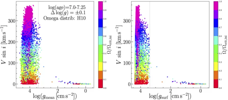
Figure 5 show the distribution of a synthetic population of 40000 stars in the υ sin i versus log g diagram, with ages distributed be-tween 10 and 18 My.
To construct this diagram, stellar models with an α=0.1 were used. The initial masses and rotations are randomly chosen so that the final distributions of the masses and rotations are equal to, respectively, the Salpeter’s Initial Mass function and the dis-tribution of the initial rotation velocities as deduced from obser-vations by Huang et al. (2010). We assumed a uniform distribu-tion of the ages between the limits indicated above and a uniform distribution of the inclinations of the rotational axis with respect to the line of sight. Inclination effect changes the perceived color and flux received from a rotating star. A fast-rotating star ap-pears brighter and bluer at the pole than at the equator. This has an impact also on surface gravity. The plotted gravity is the flux weighted (∼ T4) average of the local effective gravity on the visible hemisphere. A star seen equator-on has a surface gravity lower than the whole surface flux averaged gravity, while a star observed pole-on will show a surface gravity that is stronger than the whole surface flux-averaged gravity.
Such plots tell us how the transition from the MS band to the more evolved stage would appear if stars in a limited range of ages would be considered. Looking at the width in log(g) of the MS band (i.e., stars with a surface log(g) larger than around 3.4), we see that for υ sin(i) values larger than 300 km s−1(the
magenta dots), the MS band becomes narrower. This is a con-sequence of rotational mixing which, at such high rotation, is
strong enough to keep the stars more compact and thus with a higher surface gravity during the MS phase.
After the MS band, there is a lack of stars in a domain be-tween about 2.5 and 3.5, indicating that the model stars evolve very rapidly in that gravity domain. This phase corresponds to the crossing of the HR gap. Then we can see again stars with low gravity (log(g) < 2.5). These stars are burning helium in their core. The position in the HRD where the core He-burning begins depends on many ingredients of the models. In the present models, the core He-burning phase begins in the red super-giant phase. Considering lower metallicities or using different prescriptions for the rotational mixing may change this picture keeping stars with a relatively high surface velocity beyond the end of the MS phase.
Considering these synthetic populations as mock observa-tions, the value of log g at which the drop in velocity occurs might be taken equal to ∼3.4 if we take the limit given by stars with υ sin i below about 100 km s−1, or equal to 3.1 if we take
the limit given by stars with υ sin i between 100 and 200 km s−1. For the ages of the synthetic clusters considered here, the ini-tial masses of the stars at the end of the MS phase are near 15 M . In the left panel of Fig. 5, we plot, as a vertical line, the limit
of the MS band for a 15 M computed with an α=0.1, an initial
rotation equal to υ/υcrit=0.4, and a moderate angular
momen-tum transport. These properties correspond to the properties of the models used to construct the synthetic population and thus the vertical line indicates the true end of the MS band in this diagram. Looking at the right panel of Fig. 5, which shows the distribution of stars for the same populations as the one shown on the left diagram, but with no inclination effect, we see that this limit perfectly matches the end of the MS band.
The best strategy to obtain the position of the true drop off (here at log g=3.4) is to take the limit given by the lowest grav-ity at which stars are more or less uniformly distributed among low and high υ sin i values. Looking at the left panel of Fig. 5, we see that for log g above 3.4, such a uniform distribution of υ sin i is realized, while below that value, a non-uniform distri-bution is obtained in the low velocity range (υ sin i < 100 km s−1). For higher υ sin i, some points appear beyond this limit. This dispersion is mainly caused by two effects, first the impact of rotation on the tracks and second the inclination effect. For moderate rotation rates, tracks end their MS phase with a slightly lower surface gravity than non-rotating tracks. This is because in this velocity range, rotation produces more massive convective cores, while not driving an overly strong mixing in the envelope that would keep the star more compact. The effect of inclination comes from the fact that a star seen equator-on would show a sur-face gravity that is smaller than the whole sursur-face flux-averaged gravity.
4.2.2. Comparison with IACOB project observations
The analysis of the sample used here, obtained within the frame-work of the IACOB project, is described in Simón-Díaz et al. (2017). With the aim to provide new empirical clues about macroturbulent spectral line broadening in O- and B-type stars to evaluate its physical origin, Simón-Díaz et al. (2017) com-piled high-quality spectra of a sample of ∼430 stars with spectral types in the range O4 – B9 (all luminosity classes). By means of a detailed quantitative spectroscopic analysis, these authors de-termined estimates of the effective temperatures (Teff), surface
gravity (log(g)), and projected rotational velocity (υ sin(i)). For the sake of including relevant information for interpreting the di-agrams presented in this section, we note that the sample of stars
Fig. 5. Synthetic populations of stars obtained by adding five clusters (computed with Syclist, Georgy et al. 2014a), each of 10 000 stars at solar
metallicity with a turn off mass around 15 M . The stellar models are from Georgy et al. (2013). These models have the same physic inputs as
the one used for computing our moderate angular momentum transport models with an α= 0.1. The range of ages spanned by the five clusters is
indicated in the left panel. A noise of ± 0.1 dex is considered in log(g). An initial distribution of rotations as given by Huang et al. (2010) is used.
The left panel shows a population with the log(g) limit determined for our 15 M model with αov= 0.1. The right panel shows the same population
but this time the correction for the angle of view is not applied on log(g).
3.5 4.0 4.5 log(Teff[K]) 2.0 2.5 3.0 3.5 4.0 4.5 log( L /L )
log(g)=4 log(g)=3 log(g)=2
7M 9M 15M 25M 3.5 4.0 4.5
log(g)=4 log(g)=3 log(g)=2
50 100 150 200 250 300 350 400 υ sin(i) [km s − 1]
Fig. 6. Positions of the stars with a determined υ sin(i) taken from Simón-Díaz et al. (2017) and Holgado et al. (2020, in prep.) in the spectroscopic HR diagram. The evolutionary tracks correspond to non-rotating tracks with an α=0.3. The left-panel shows the mass selection and the right panel shows the υ sin(i) distribution.
investigated by Simón-Díaz et al. (2017) was limited to cases not identified as double-line spectroscopic binaries (SB2) and hav-ing a υ sin(i) <200 km s−1.
The sample of Galactic OB stars considered by Simón-Díaz et al. (2017) was recently updated with a sample of (285) likely single O-type stars (this time including the full range of υ sin(i) values). In this case, spectroscopic parameters were presented in Holgado et al. (2020), and υ sin(i) results are soon to be pub-lished (Holgado et al., in prep.)7. Again, for a better
understand-ing of the diagrams presented in this section, we remark that the sample of stars investigated by Holgado et al. (having all of the
7 Results for half the sample are already available in Holgado et al.
(2018).
masses above 20 M ) covers the full range of υ sin(i) values (up
to ∼450 km s−1).
The complete sample of stars is plotted in a spectroscopic HR diagram in Fig. 6. The sample only populates the region from the ZAMS down to log(Teff) ∼ 4.1 since this is the domain in the
sHRD where O and B stars – the main type of targets surveyed by the IACOB project – are located.
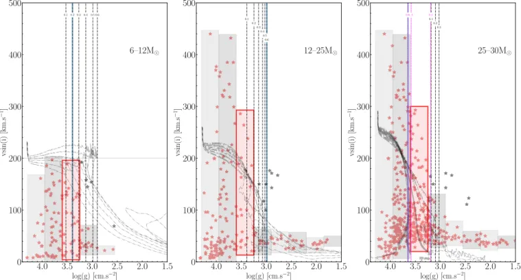
Figure 7 shows the surface velocity versus surface gravity diagrams for rotating models for three different bins in mass. In all cases, we also include model predictions for models with various α values for a characteristic mass, and those empirical results corresponding to subsamples of stars fulfilling the mass range criteria (see Fig. 6). The leftmost panel of Fig. 7 contains all stars shown in black and red in Fig. 6, that is, those aggregat-ing around the 7 and 9 M models. We overplotted the tracks for
our 9 M with υ/υcrit=0.4 (moderate angular momentum) and
different overshoots. The surface velocity for the track is the ac-tual (non-projected) equatorial velocity. For the observed points, υ sin(i) is indicated. This implies that the positions of the ob-served stars whose actual surface velocity would be equal to that of the model are on or below the tracks. The middle panel shows data points corresponding to higher initial masses (green and blue points in Fig. 6). The tracks are those of the present work for 15 M (otherwise the same physics inputs as for the tracks shown
on the left panel). The right panel shows points corresponding to even higher masses (blue points and grey points above) overplot-ted on 25 M tracks (same physics inputs as other panels).
In the observed sample, we do not expect to see the sharp drop in number beyond the MS phase. Indeed looking at Fig. 6, we do not see any sharp drop in the number of stars in the e ffec-tive temperature range covered. Thus, here the feature that is to be compared with the theoretical prediction is the drop in surface velocity, not the drop in the number of stars. In this regard, we remark again that, as indicated above, the sample of stars con-sidered in the leftmost panel of Fig. 7 only includes stars with
1.5 2.0 2.5 3.0 3.5 4.0 log(g) [cm.s−2] 0 100 200 300 400 500 vsin(i) [km.s − 1] 6–12M 0.1 0.2 0.30.40.5 0.6 1.5 2.0 2.5 3.0 3.5 4.0 log(g) [cm.s−2] 0 100 200 300 400 500 vsin(i) [km.s − 1] 12–25M 0.1 0.2 0.3 0.4 0.5 0.6 1.5 2.0 2.5 3.0 3.5 4.0 log(g) [cm.s−2] 0 100 200 300 400 500 vsin(i) [km.s − 1] 25–30M 0.1 0.2 0.3 0.4 0.5 0.6
Fig. 7. Comparison of observed and predicted surface velocities as a function of surface gravity. In each panel, the light grey dashed tracks show the evolution for a given initial mass model of the surface equatorial velocity as a function of the surface gravity, with overshooting equal to 0.1, 0.2, 0.3, 0.4, 0.5, and 0.6 (from left to right, except for the right panel, where models, due to blueward evolution at α ≥ 0.4, goes as
0.6,0.5,0.4,0.1,0.2,0.3 from left to right). The models have been computed with υ/υcrit= 0.4 and a moderate angular momentum transport. Models
with an initial mass equal respectively to 9, 15, and 25 M are plotted in the left, middle, and right panel. The vertical lines shows for each
overshooting value, the value of the log(g) where the expected υ sin(i) drop is predicted to occur. The one shadowed in blue shows the case corresponding to the model with the overshoot deduced from the MS band’s width (see Sect. 4.1). The colored stars are observed υ sin(i) given by Simón-Díaz et al. (2017) catalogue and brand new O-star sample with high υ sin(i) from Holgado et al. (in prep.). For the mid/late B-stars,
Simón-Díaz et al. (2017) excluded from their sample all stars with υ sin(i) >200km s−1to study macroturbulent broadening (hatched zone in the
left panel) . In each panel, we plot only those stars showing a position in the HR diagram indicating that they have a mass near the one of the plotted stellar models. In each panel, the red band indicates the region where the υ sin(i) drop likely occurs. To determine its position, we use both observations and considerations based on the mock observations shown in Fig. 5 (see text). In that process, however, we do not take into account the grey stars that, according to Holgado et al. (in prep.; see Fig. 1 in Britavskiy et al. 2020), might be the result of the evolution of an interacting binary system.
υ sin(i)<200 km s−1, an empirical bias which also partially
af-fects the middle panel, but not the rightmost panel.
For the purposes of comparison, we binned the data points. The width of the bins in logg (here 0.35 dex) is a compromise between reaching a sufficiently good resolution in log(g) and at the same time having a sufficient number of points in each bin to appropriately derive a meaningful mean value for υ sin i. We tested other widths of the bins and obtained the same results as those quoted here.
We colored in blue the vertical line showing the end of the MS band corresponding to the value of α as deduced from the discussion in Sect. 4.1. In the following, we ignore the grey stars for determining the υ sin(i) drop since according to de Burgos et al. (in prep.), these stars might result from the evolution of interacting binary systems.
As discussed in Sect. 4.2.1, as the end of the MS band we chose the last bin before the observed υ sin(i) drop, where the υ sin(i) are still distributed continuously over a large range. In each panel of Fig. 7, we highlighted this bin in red.
First, in the case of stars with masses around 6–12 M (left
panel of Fig. 7), the third bin (from the left) seems like the most appropriate choice with this method. The value derived from the MS width band is compatible with this result. This leads to the
conclusion that in the 6–12 M mass range, an α between 0.1
and 0.3 seems appropriate.
For the case of the stars with higher initial masses, between 12–25 M (see the middle panel of Fig. 7), using the same
method, we obtain an overshooting α between 0.1 and 0.2 (see the bin highlighted in red). These values are thus smaller than those derived from the MS width.
Finally, let us consider the last mass range, 25–30 M (see
the right panel of Fig. 7). The 25 M models with α > 0.4 enter
into the Wolf-Rayet phase during the MS phase and thus show an evolution towards a higher surface gravity during the MS phase (see the first two tracks starting from the left in the third panel). Thus, a high α value already produces WR stars over the duration of the MS phase from 25 M models with an initial rotation that
is moderate. This would likely produce too many WR stars (from single stars) with respect to what has been observed. Thus, such high values of α do not appear reasonable and we do not consider them here. The third bin (from the left) seems an appropriate choice for the υ sin(i) drop. Taken at face value, this would point either to an α value between 0.4 and 0.5 or to an α value around 0.1. If we discard the value of 0.5, then remain two possibilities, either 0.1 or 0.4. At the moment, a conservative approach would be to stick to the value obtained in the 12-25 M range.
In summary, for the mass range below ∼12 M , the surface
velocity drop method gives a range of values for α compatible with the one given by the method based on the width of the MS band. For the mass range above ∼12 M , the values of the
over-shooting parameter α obtained from the υ sin(i) drop are lower than the ones obtained from the MS width. In this mass range, we currently favor the results given by the velocity drop over the one coming from the spectroscopic HR diagram. The main rea-son for this is that in the upper HR diagram (for masses above ∼ 12 M ), the observations do not yet provide a well-defined
posi-tion for the drop in the density of stars. In light of all the above, we suggest a value of α=0.1 for 7 M and α=0.2 for masses
be-tween 9 to 25 M . Interestingly, this choice appears to be
con-firmed by the results obtained by Tkachenko et al. (2020) using eclipsing binaries (see the discussion in Sect. 5).
4.3. Synthesis of these comparisons with the observations In summary, we obtain from the comparisons made in the above sections the following values of α:
(1) α= 0.1 for masses between about 2 and 7 M ;
(2) α= 0.2 for 9 M ;
(3) For 15 M and 25 M models, we suggest α= 0.2 as a
conservative choice, but other options are possible as seen in the precedent sections.
The values of α given above are only valid for the physic in-puts of the considered models. The convective core sizes appear to increase more rapidly with the mass than given by models with a constant step overshoot α=0.1. We find here a moderate increase of α with the mass occurring between 7 and 9 M . In
the next two sections, we first discuss the robustness and the lim-itations of these results and indicate some perspectives for future works in this area of research.
5. Discussion
5.1. Limitations of the different methods
Each of the methods has its own specific limitations. At least two limitations are generic to all methods: the first one, is that whatever the observed feature considered, these features depend on more physical processes than just convection. Mass loss by stellar winds and transport in the radiative zones are, for in-stance, two important processes that also affect the position of the TAMS in the HR diagram and of the surface gravity at which the velocity drop occurs. The second one comes from the relia-bility of the parameters derived from the observed sample.
5.1.1. Width of the MS band
For the MS width, one of the main limitations comes from the difficulty in the upper part of Fig. 4 to find the position of the end of the MS band as a clear drop of the stellar density. The situation is much better in the lower mass range. Thus the results obtained for masses between 7 and ∼15 M are likely more reliable than
those for higher masses. Another difficulty comes from the fact that unresolved binaries can actually populate an area beyond the TAMS predicted by single-star models (Wang et al. 2020). We note, however, that some of the stars in Castro et al. (2014) not identified as SB2 could still be SB1 systems or mergers. Hence, it is difficult to be completely sure that we have eliminated all binaries in the sample. The same applies to the two other samples (Simón-Díaz et al. 2017, Holgado et al. 2020).
5.1.2. Velocity drop
In the observed sample used here, there is an important ob-servational bias for the mid and late B-stars since Simón-Díaz et al. (2017) excluded from their sample all stars with υ sin(i) >200km s−1to study macroturbulent broadening.
More-over, the B-MS stars are highly biased towards low υ sin(i) stars due to their interest in determining abundances in the Solar neighborhood. In this case, we note that the sample for the 7-9 M would need to be more populated (both in high υ sin(i) for
MS stars, and low υ sin(i) for post-MS stars) to better constrain the α value. The situation is better for the mass range of 15 and 25 M .
Another major difficulty comes from the effect of binaries and of inclination that blurs the picture. Stars resulting for in-stance from a merger may have a surface rotation very different from the one predicted by single star evolution. Inclination effect may populate regions beyond the end of the MS band with fast rotating MS stars. In that case, the positions of these fast-rotating stars in the υ sin i versus log g diagram do not necessarily require a larger convective core to be fitted but at least an appropriate ac-count for the effects of inclination on their surface properties.
In the present models, we used the same mass loss prescrip-tions as in Ekström et al. (2012). These mass loss recipes account for the bistability effects. This effect, found by Vink et al. (2010), results in a rapid and strong increase of the mass loss by stellar winds when some limits to effective temperatures are reached. If this happens before the end of the MS phase, it may produce a drop in the surface rotation that can be wrongly interpreted as having been due to the expansion of the star at the end of the MS phase. We checked that the drop in velocity shown by our stellar models is due to the expansion of the star after the MS phase and not to this bistability effect. Such an effect can occur before the end of the MS phase in faster-rotating models than those con-sidered here. Typically stars should rotate faster than 70% of the critical velocity. Such fast rotators are very rare and thus cannot explain the drop seen in Fig. 7.
5.2. Impact of different physical ingredients for the models In the present work, we considered extending the convective core above the limit given by the Schwarzschild limit. We may won-der whether the results would be different if we had chosen to extend the convective core above the limit given by the Ledoux limit. During the MS phase, we do not expect any difference. Indeed, since the core is decreasing in mass, there is no chem-ical composition gradient at the border of the convective core and, hence, there is no difference between the Schwarzschild and Ledoux criteria. Differences appear, of course, during the core He-burning phase, where the convective core is increasing in mass. Thus changing from the Ledoux to the Schwarzschild criterion has an impact on the extension of the blue loops, on the changes of the surface abundances, and on the sizes of the inter-mediate convective zones (occurring during the core He-burning phase, see e.g., the discussion in Georgy et al. 2014b, Kaiser et al. 2020) but, of course, not on the observed features linked to the core H-burning phase.
We consider here the extension of only the convective cores. We could have considered applying an overshoot to all convec-tive zones (intermediate, outer convecconvec-tive zones). During the MS phase, there are no significant intermediate convective zones, nor convective envelope, thus our choice to discard models with overshooting for intermediate convective zones or convective en-velopes is not a strong limitation of the present work.
Interme-diate convective zones and an outer convective zone, in general, appear during the core He-burning phase.
In this work, we focused on step overshooting while other studies use a diffusive approach for the mixing of the chemical elements in the overshooting region. Depending on which ap-proach is used, the gradients of chemical composition at the bor-der of the core unbor-dergo modification: very steep gradients are expected for the step overshooting (if acting alone) and much smoother gradients in case of the diffusive approach. Asteroseis-mology can in some cases probe the structure of the chemical gradients at the border of the convective core and thus provide some hints favoring one over the other among these two ap-proaches. We did not consider the diffusive overshooting type here but we do discuss rotating models that actually produce both an extension of the convective core (due to another phys-ical process than overshooting) and a smoothing of the chemphys-ical gradients just above the core. Thus, to some extent, while it may be for a different physical reason, these rotating models cover (at least in a qualitative sense) the cases of models that would have been computed with a diffusive overshoot. We note however that since the physical process at work are different, the value for α that that would be deduced from non-rotating diffusive over-shooting models and the values deduced from the present rotat-ing step-overshoot models are likely to be different. On the other hand, diffusive overshooting models would likely also require an increase of the overshoot with the mass. This is indeed what we see when we look at our rotating models that require such an increase.
In addition to the two cases of moderate and strong angu-lar momentum transports considered here, many other different ways of accounting for the effects of rotation exist. A limited study of the impact of different prescriptions for the shear dif-fusion coefficient and the horizontal diffusion coefficient can be found in Meynet et al. (2013). However, the cases discussed here (υ/υcrit = [0, 0.2, 0.4], α=[0.1,...,0.6] and Sr/Mo transport)
ex-plore more extreme situations in term of angular and chemical element transports than those explored in the above reference. Thus, it is quite possible that present models cover all the situ-ations (and even more) resulting from these different prescrip-tions.
So, on the whole, the values quoted at the end of Sect. 4 for α do not appear to be too much dependent on the fact that we chose the Schwarzschild instead of the Ledoux criterion, whether over-shoot is implemented or not for modifying the extension of inter-mediate or external convective zone. They also do not appear to be too strongly dependent on the two types of angular momen-tum transport considered in this work (moderate or strong). This last point has to be taken with some caution. We have seen that the two types of models are similar for moderate initial rotation but may differ significantly for fast-rotating models.
5.3. Comparisons with other models
We make use of the models discussed in Tkachenko et al. (2020) to briefly make a comparison between the core sizes they obtain with those presented here. These authors have used 11 eclips-ing binaries with masses of the components between 4 and 16 M to determine the convective core size during the core
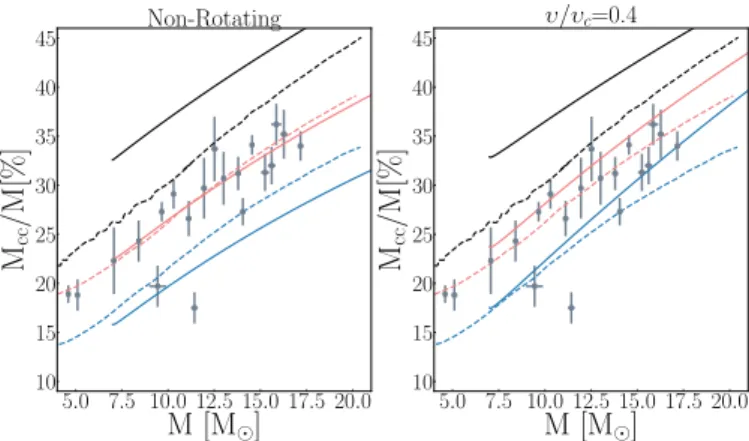
H-burning phase. In Fig. 8, we compare the size of the convec-tive cores obtained at the middle of the MS phase with those obtained by Tkachenko et al. (2020). We see that the line cor-responding to our non-rotating model with α=0.2 nearly per-fectly matches their line corresponding to a strong convective boundary mixing, which is their favored model. For the
rotat-5.0 7.5 10.0 12.5 1rotat-5.0 17.5 20.0 M [M ] 10 15 20 25 30 35 40 45 Mcc /M[%] Non-Rotating 5.0 7.5 10.0 12.5 15.0 17.5 20.0 M [M ] 10 15 20 25 30 35 40 45 Mcc /M[%] υ/υc=0.4
Fig. 8. Variation of the convective core size at different stages during the core H-burning phase, as a function of the initial mass. The dashed lines are the models of Tkachenko et al. (2020) with strong convective boundary mixing, the solid ones are the present GENEC models with α=0.2. The tracks in black correspond to the ZAMS stage, while the red tracks correspond to a stage where the mass fraction of hydrogen in
the convective core (Xc) is 0.35, and the blue tracks to Xc=0.1. The grey
points show observed eclipsing binaries and their core mass estimates from Tkachenko et al. (2020). In the left panel, the GENEC models are
the non-rotating ones. In the right panel, they are the υ/υcrit=0.4 rotating
ones.
ing models, models with α between 0.1 and 0.2 would match their line, which is obtained with a strong boundary mixing. In-terestingly, the slope of the variation of the core mass with the mass is very similar in models with a constant step overshoot and the ones with a convective boundary mixing as implemented in Tkachenko et al. (2020). These comparisons illustrate the fact that comparing predictions of stellar models with observations as those above cannot constrain the mixing at the boundary of the core; however, they can provide insights on the size of the convective core, whatever the physical process responsible for it (boundary mixing, overshoot, rotation). We see here that adopt-ing a value of α around 0.2 for masses up to 16 M would
pro-vide a good fit to the models, which, according to Tkachenko et al. (2020), best match the constraints from their sample of eclipsing binaries.
6. Conclusions
The main findings of the present works are the following: – We discuss the impact of different overshooting values on
two observed features and within the framework of three dif-ferent types of models: non-rotating, rotating with a moder-ate angular momentum transport, rotating with a strong an-gular momentum transport.
– A constant α value (here α=0.1) for a step-overshoot be-tween ∼2 and ∼ 7 M allows us to adequately fit the observed
TAMS and the observed drop of the surface velocity. – We confirm, as found by earlier works and other works in
progress (Castro et al. 2014, Scott et al. submitted) that for more massive stars, there is a need to consider an α value that increases with the mass.
– The increase of α with the mass that we can deduce from comparisons of the present stellar models with the position of the TAMS and from the position of the velocity drop is not of the same amplitude. A larger increase is obtained from the MS band width. However, in the upper mass range, the TAMS position coming from the observations is not easy to