OSCILLATIONS MILLÉNAIRES DES CONDITIONS HYDROGRAPHIQUES D'ISFJORDEN, OUEST DU SPITZBERG, AU COURS DE L'HOLOCÈNE, EN RELATION AVEC LA DYNAMIQUE DE LA DÉRIVE NORD-ATLANTIQUE
MÉMOIRE PRÉSENTÉ
COMME EXIGENCE PARTIELLE
DE LA MAÎTRISE EN SCIENCES DE LA TERRE
PAR CAMILLE BRICE
Service des bibliothèques
Avertissement
La diffusion de ce mémoire se fait dans le respect des droits de son auteur, qui a signé le formulaire Autorisation de reproduire et de diffuser un travail de recherche de cycles supérieurs (SDU-522 - Rév.01-2006). Cette autorisation stipule que «conformément à l'article 11 du Règlement no 8 des études de cycles supérieurs, [l'auteur] concède à l'Université du Québec à Montréal une licence non exclusive d'utilisation et de publication de la totalité ou d'une partie importante de [son] travail de recherche pour des fins pédagogiques et non commerciales. Plus précisément, [l'auteur] autorise l'Université du Québec à Montréal à reproduire, diffuser, prêter, distribuer ou vendre des copies de [son] travail de recherche à des fins non commerciales sur quelque support que ce soit, y compris l'Internet. Cette licence et cette autorisation n'entraînent pas une renonciation de [la] part [de l'auteur] à [ses] droits moraux ni à [ses] droits de propriété intellectuelle. Sauf entente contraire, [l'auteur] conserve la liberté de diffuser et de commercialiser ou non ce travail dont [il] possède un exemplaire.»
Je tiens à remercier en premier lieu ma directrice Anne de Vernal qui rn' a aidée, guidée et encouragée depuis le baccalauréat jusqu'à aujourd'hui. Je la remercie d'avoir toujours été présente pour me soutenir tout au long de mon cheminement académique, surtout durant les moments les plus difficiles. Toutes les opportunités qu'elle m'a offertes, entre les expéditions en mer et les congrès à l'international, rn' ont énormément formée et ont transformé cette maîtrise en une expérience inoubliable. Merci aussi à mon codirecteur Pierre Francus de m'avoir accueillie dans son laboratoire à Québec. Je dois le remercier pour ses connaissances en sédimentologie et pour le partage de ces dernières avec moi. Un grand merci à Matthias Forwick sans qui mon stage à Troms0 n'aurait jamais eu lieu. Mon séjour en Norvège m'a permise de me former en laboratoire, mais aussi de vivre une belle aventure à l'international. Je remercie Matthias d'avoir pris le temps, malgré son horaire très chargé, de m'accueillir et de m'aider durant ce temps et aussi tout au long de mon projet.
Merci à tous les merveilleux étudiants et membres ArcTrain et Geotop. Merci d'avoir écouté mes présentations orales et regardé mes posters à toutes les années. Mais surtout, je n'oublierai pas tous les congrès, les pots, les partys d'Halloween, les Annual Meetings. . . qui ont été dans les meilleurs moments de ma maîtrise, durant lesquels j'ai fêté et rencontré des personnes incroyables. Merci à mes amis tri peux de plein air et de roches avec qui je peux toujours partir à l'aventure. Une belle pensée pour Dominique (et Miette évidemment) qui rend ma vie beaucoup plus fun et agréable.
Comment survivre dans le laboratoire de micropaléontologie sans la magnifique dame Estelle ? Un énorme merci à cette incroyable responsable de lab qui nous a gardé en vie et en ordre les dernières années, mais surtout un merci à ma grande amie d'être dans ma vie et sans qui le 7e étage serait vraiment plus plate. Et finalement, je pense à ma merveilleuse amie Jade. Celle avec qui j'ai eu la chance de partager le laboratoire et les microscopes pendant d'innombrables heures, à mimer les dinokystes,
à danser dans l'habit de HF ou encore à rire jusqu'à en pleurer. Je la remercie pour rn' avoir aidée tant pendant le bacc. que pendant la maîtrise, en me rappelant quel est mon objectif, en relisant mes textes ou simplement en étant une amie.
Un grand merci à ma famille de toujours m'encourager dans mes démarches et d'être présente et fière de moi. Un merci spécial à ma sœur Marie-Hélène et à Kevin de m'avoir grandement aidé dans mes analyses statistiques. Sans leur générosité et leur patience, je n'aurais pas pu réaliser tout ce que je voulais pour mon projet. Et pour terminer, le plus grand des mercis à ma belle Alice. Merci d'avoir fait des allers-retours Québec-Montréal, merci pour tes incalculables visites dans mon bureau, merci d'accepter mes sautes d'humeur, merci d'être aussi drôle. Bref, merci de faire partie
Ce projet de recherche s'inscrit dans le cadre d'une collaboration avec l'Université de Troms0 (UiT), l'Institut de recherche polaire de Corée (KOPRI), l'Institut National de la Recherche Scientifique et l'Université du Québec à Montréal. Le prélèvement de la carotte à l'étude HH16-1205-GC a été fait à bord du navire de recherche Helmer Hanssen de l'UiT par Matthias Forwick (UiT) et Seung-Il Nam (KOPRI). Les analyses granulométriques ainsi que les analyses sur le carbone organique ont été réalisées par Seung-Il Nam. J'ai contribué au projet en réalisant les mesures géochimiques et physiques, la description lithologique et les analyses palynologiques.
Le mémoire a été construit sous forme d'article scientifique et sera soumis à la revue
Boreas prochainement. L'article, soit le chapitre 1 du mémoire, est donc rédigé en
AVANT-PROPOS ... v
LISTE DES FIGURES ... ix
LISTE DES TABLEAUX ... xiii
LISTE DES ABRÉVIATIONS ... xv
LISTE DES SYMBOLES ... xvii
RÉSUMÉ ... xix
INTRODUCTION ... 1
CHAPITRE I MILLENNIAL-SCALE OSCILLATIONS OF HYDROGRAPHie CONDITIONS IN ISFJORDEN, WEST SPITSBERGEN, DURING THE HOLOCENE, IN RELATION TO THE NORTH-ATLANTIC DRIFT DYNAMICS 5 ABSTRACT ... 7 1.1 Introduction ... 9 1.2 Study are a ... 11 1.2.1 Physiographic setting ... 11 1.2.2 Geology ... 12 1.2.3 Oceanography ... 12 1.3 Methodology ... 14 1.3 .1 Sedimentology ... 14 1.3.2 Chronology ... 16 1.3.3 Microfossils analysis ... 16
1.3 .4 Reconstruction of sea surface conditions ... 17
1.3 .5 Time-series analysis and quantitative treatment ... 18
1.4.1 Chronology ... 19 1.4 .2 Physical properties ... 19 1.4.3 Geochemistry ... 20 1.4.4 Palynology ... 22 1.4.5 Statistical analysis ... 24 1.5 Discussion ... 27
1.5.1 Holocene transitions and major changes ... 27
1.5.2 Mode ofvariability ... 31
1.5.3 Cross-correlation between sedimentological and palynological data ... 34
1.6 Conclusion ... 36
1. 7 References ... 3 7 CONCLUSION ... 63
ANNEXE A RÉSULTATS GÉOCHIMIQUES COMPLÉMENTAIRES ... 67
ANNEXE B RÉSULTATS GRANOLUMÉTRIQUES COMPLÉMENTAIRES ... 71
APPENDICE A RÉSULTATS DES ANALYSES PAL YNOLOGIQUES ... 73
APPENDICE B RÉSULTATS DES ANALYSES SÉDIMENTOLOGIQUES ... 85
APPENDICE C PHOTOGRAPHIES DE LA CAROTTE HH16-1205-GC ... 107
Figure Page
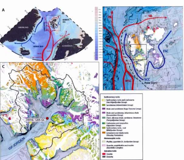
Figure 1. 1 Maps of the study area. A: Map of the North Atlantic. Red arrows
represent the North Atlantic drift with Irminger Current (IC), Norwegian
Atlantic Current (NwAC), Norwegian Atlantic Slope Current (NwASC), North Cape Current (NCaC), West Spitsbergen Current (WSC), Svalbard Branch (SB) and Y ermack Branch (YB). The blue arrows represent the Arctic water flowing via East Spitsbergen Current (ESC) and East Greenland Current (EGC). Green arrows are the Norwegian Coastal Current (NCC). White line indicates the mean
position of the Polar Front (Loeng, 1989). B: Geological map of Svalbard (data
from Norwegian Polar Institute and International Bathymetrie Chart of the Arctic Ocean) with the South Cape Current (SCC). Dashed line represents the general position of the polar front. C: Geological map of Isfjorden with location
of the core. Plain black line is the main watershed boundary; dotted lines are
secondary watershed limits. Df: Dicksonfjorden, Bf: Billefjorden, Sf:
Sassenfj orden ... 51
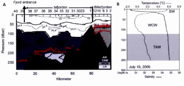
Figure 1. 2 Conductivity, temperature, depth (CTD) profiles of Isfjorden. A W:
Atlantic Water, TA W: Transformed Atlantic Water, WCW: Winter Cooled
Water, LW: Local Water, SW: Surface Water. A: CTD section from Billefjorden toward Isfjorden mouth along the southem side of the fjord in September 2002. Modified from Nilsen et al. (2008). B: CTD profile taken in 2005 at the site of
core JM98-845-PC (78°20.64' N; 15°18.11' E), close to core HH16-1205-GC
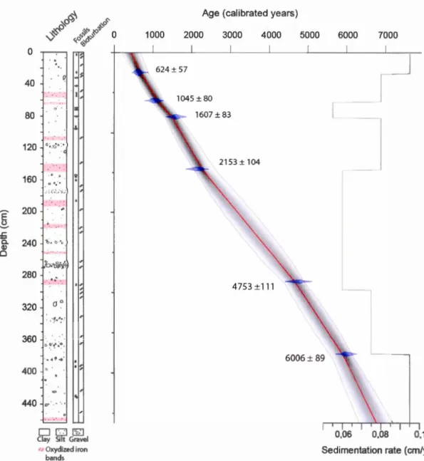
Figure 1. 3 Lithological description, age-depth profile and sedimentation rate of core HH16-1205-GC. Age vs. depth relationship was modeled with R package
BACON based on 14C chronological dates ... 54
Figure 1. 4 Grain size distribution mode, density and magnetic susceptibility,
8 13Corg, percentage of total organic carbon (TOC), ratio of carbon versus
nitrogen (C/N) and percentage of carbonates (CaC03) in bulk sediment of core
HH16-1205-GC ... 55
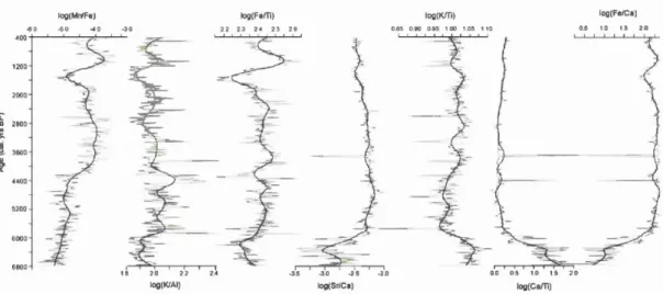
Figure 1. 5 Geochemical content in sediment of core HH16-1205-GC expressed
as elements log-ratios ... 56
Figure 1. 6 Concentration of dinocysts and Halodinium and percentages of the
main dinocyst taxa in core HH16-1205-GC. Species written in red are phototrophic and those in blue are heterotrophic ... 57
Figure 1. 7 Sea surface conditions reconstructed from the application of MAT to
the dinocyst assemblages of core HH16-1205-GC. Sea surface temperatures (SST) in summer and winter are represented by red and blue curves respectively. Summer and winter sea surface salinities are shown by the red and blue curves, sea ice cover and annual productivity are represented by purple and green lines
respectively. Black curves correspond to smoothed values after Loess
regressions ... 58
Figure 1. 8 Results pf multivariate analysis of the environmental and
geochemical variables, and the dinocyst taxa percentages. A) Principal component analysis of XRF ratios and sea surface parameters. B) Redundancy analysis of sea surface parameters and dinocysts taxa percentages. C) Regression analysis ofXRF ratios and dinocyst taxa percentages ... 59
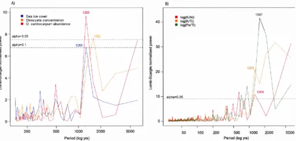
Figure 1. 9 Periodicity of (A) reconstructed sea ice cover, dinocyst concentration
and relative abundance of Operculodinium centrocarpum and (B) XRF
log-ratios KI Al, K./Ti and Fe/Ti computed from a Lomb-Scargle periodogram.
Significance levels (alpha) were established at 5o/o (A and B) and 10o/o (A). Peak
values are 1265 years for sea ice cover and Operculodinium centrocarpum and
1582 years for dinocyst concentrations, 1269 years for K./Al and K/Ti and 1587
years for Fe/Ti ... 60
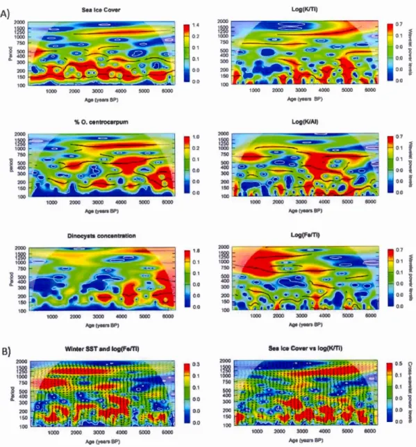
Figure 1. 10 Spectral analysis of the time series. (A) Wavelets analysis applied
on MAT reconstructions, palynological results and XRF data. (B)
Cross-wavelets analysis between ratios (K/Ti, Fe/Ti) and sea surface conditions ... 61
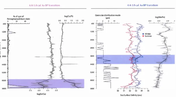
Figure 1. 11 Results of the mmn prox1es characterizing the two maJors
Tableau Page
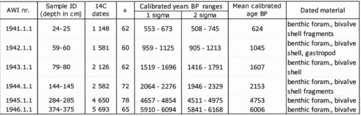
Tableau 1.1 Radiocarbon dates of core HH16-1205-GC and corresponding calibrated ages. The calibration was made with a ~R of 90 ± 35 on BACON with the Marine 13 calibration curve ... 50
AMOC AMS
BP
Cal. a cf e.g. ca.Atlantic meridional overturning circulation
Circulation méridienne de retournement de 1 'Atlantique
Accelerator mass spectrometry
spectrométrie de masse par accélération
Before present Avant 1' actuel Calibrated year Année calibrée Confer Se reporter à Exempli gratia Par exemple Circ a Près de
cm psu SI Environ Degrés Celcius centimètre
Unité de salinité (practical unit salinity)
Unité de susceptibilité magnétique, valeurs exprimées en masse spécifique
Les fjords de la côte Ouest du Spitzberg sont des endroits reliant le milieu continental
au milieu marin qui enregistrent ainsi 1' interaction entre les eaux atlantiques, la glace
de mer et les glaciers. Les branches les plus nordiques de la dérive nord-atlantique
transportent jusque dans l'Océan Arctique un flux de chaleur, qui limite l'étendue de
glace de mer et contrôle le bilan d'énergie entre l'océan et l'atmosphère. L'étude
d'une archive sédimentaire (la carotte HH16-1205-GC) du plus grand système de
fjord du Spitzberg, Isfjorden, a permis de retracer les variations des conditions
hydroclimatiques au cours des derniers 6800 ans.
La période couverte par 1' enregistrement couvre de 1 'Holocène moyen à supérieur qui
se caractérise par un refroidissement graduel. Deux phases de refroidissement plus marqués sont enregistrées. Un environnement de glaciers proximaux avec une activité
glaciaire importante, des eaux stratifiées mais aussi une productivité primaire élevée
caractérisent une première phase de 1000 ans de la carotte, soit de ~ 6800 à 5800 ans
BP. À ~ 4000 ans BP, la précipitation de manganèse indique que le milieu devient
plus anoxique, probablement en relation avec une diminution de l'intensité du courant
profond dans le fjord. Les eaux atlantiques formant la masse d'eau intermédiaire à
profonde à cet endroit, la diminution de son advection dans le fjord pourrait avoir
causé une anoxie du milieu. Durant l'intervalle de 2000-1200 ans BP, l'augmentation
en abondance de deux espèces de dinokystes phototrophes, soit Spiniferites elongatus
et Impagidinium pallidum, révèle un environnement lègèrement plus chaud et salin.
Durant cette même période, 1' environnement redevient aussi plus oxygéné.
Superposées au refroidissement à long terme de l'Holocène, des oscillations des
conditions hydrographiques et de la composition des sédiments sont enregistrées. Ces
oscillations sont d'échelle millénaire, les périodes variant entre 1100 et 1500 ans. Le
couvert de glace présente la variabilité la plus distincte, avec une périodicité
d'environ 1250 ans qui est aussi présente dans l'abondance relative
d' Operculodinium centrocarpum et dans les ratios géochimiques K./Ti et KI Al. Des analyses par ondelettes ont confirmé ce mode de variabilié et indiquent que les
oscillations varient légèrement de l'Holocène moyen à l'Holocène supérieur et
Mots clés : Spitzberg, dérive nord-atlantique, Holocène, couvert de glace,
Plusieurs études récentes ont démontré que 1' Arctique est la région la plus sensible
aux variations climatiques actuelles (IPCC, 2014). Différents mécanismes de
rétroactions provoquent un réchauffement deux fois plus rapide que la moyenne
globale; ce phénomène est nommé l'amplicification arctique (Serreze and Barry,
2011 ). Le réchauffement accéléré de 1' Arctique a des répercussions directes sur le
système climatique du globe. Des expériences de modélisation tentent de reproduire
ce phénomène, d'évaluer la responsabilité de l'activité humaine et ainsi de prévoir
quel sera le climat dans le futur. Toutefois, la variabilité climatique naturelle, en
particulier dans les hautes latitudes, reste mal comprise. C'est pourquoi l'étude de
l'évolution du climat des régions nordiques au cours de l'Holocène est importante
( e.g., Renssen et al., 2005). Les enregistrements instrumentaux étant trop brefs pour
comprendre comment le système climatique répond aux grands changements des
forçages naturels et anthropiques, des enregistrements de longue durée à partir de
traceurs indirects du climat sont très utiles.
Les eaux nord-atlantiques, relativement chaudes et salées, proviennent des basses
latitudes et sont transportées vers le nord pour atteindre 1' Océan Arctique via le détroit de Fram et la mer de Barents (figure 1.1). Elles représentent la plus importante
source de chaleur de l'Océan Arctique (Aagaard et al., 1985). Une variation de
l'intensité ou des propriétés de ces masses d'eau influencent donc grandement le
climat de la région arctique. En effet, les eaux nord-atlantiques contrôlent en majeure
partie les limites du couvert de glace, lui même modifiant 1' albedo et les échanges de
L'archipel de Svalbard, situé entre le détroit de Fram et la mer de Barents, est au centre des interactions entre les eaux atlantiques, les eaux arctiques et la limite de la
glace de mer. La marge ouest du Spitzberg, la plus grande île de 1' archipel, est sous
l'influence directe de ces masses d'eau puisque que les courants Ouest (atlantique) et
Est (arctique) du Spitzberg la longent (figure 1.1). Par conséquent, les fjords situés
sur la côte ouest du Spitzberg sont des zones d'étude particulièrement intéressantes.
Les enregistrements sédimentaires qu'ils renferment fournissent de l'information sur
les apports en eau atlantique, la variation de la glace de mer et la position des glaciers
continentaux adjacent s'il y a lieu. L'interaction océan-glaciers peut entraîner une
réponse climatique régionale (Hald et al., 2011 ). De plus, les forts apports en
sédiment dans les fjords, dus à l'érosion continentale, permettent des enregistrements
sédimentaires à haute résolution (Svendsen et al., 1992; Hald et al., 2004, 2011;
Forwick et Vorren, 2007, 2009; Baeten et al., 2010; Forwick et al., 2010; Rasmussen
et al., 20 12).
Plusieurs études ont été réalisées dans les fjords de Svalbard notamment afin de caractériser la dernière déglaciation de la calotte glaciaire Svalbard et de la mer de
Barents (Hald et al., 2004, 2011; Forwick et al., 2010; Baeten et al., 2010;
Rasmussen et al., 2012; Bartels et al., 2017, 2018). Les fjords représentent en effet
les principales voies de drainage des glaciers (Ottesen et al., 2007). Les
reconstitutions ont essentiellement été faites à partir de traceurs des masses d'eau
profondes et intermédiaires, par exemple les populations de foraminifères (Kucera,
2007; Jorissen et al., 2007). Les données concernant les conditions des eaux de
surface sont beaucoup plus limitées ainsi que les connaissances sur les échanges entre
les différentes masses de la colonne d'eau. De plus, les enregistrements remontant
jusqu'à la déglaciation montrent de grands changements océaniques, qui peuvent
Dans cette perspective, ce mémoire a pour objectif de reconstituer les conditions
océaniques et clin1atiques d'Isfjorden, le système de fjords le plus important de
Svalbard, au cours de l'Holocène moyen et supérieur. Une approche multi-traceurs a
été utilisée afin de pouvoir retracer 1 'histoire glaciaire du Spitzberg, reconstruire les
conditions des eaux de profondeur et de surface du fjord pour, par la suite, identifier
les liens entre la dynamique de glaciers et de la glace de mer, et des conditions
océaniques de l'Atlantique Nord. L'analyse d'une carotte de sédiment prélevée dans
le centre d'Isfjorden a permis de réaliser les mesures. L'évolution de la dynamique
des glaciers et des masses d'eau profondes a pu être retracée par des analyses
non-destructives des propriétés physico-chimiques des sédiments. Les intruments utilisés
incluent un scanneur de fluorescence à rayon-X (XRF) mesurant la composition
géochimique et le Mu! ti Sens or Core Logger (MSCL) pour déterminer la densité et la
susceptibilité magnétique. Des analyses destructives telles que la granulométrie et la palynologie ont aussi été réalisées. Les reconstitutions des conditions des eaux de
surface ont été faites à 1' aide de la technique des analogues modernes (Modern
Analogues Technique; MAT; Guiot et de Vernal, 2007) à partir d'assemblages de
kystes de dinoflagellées ( dinokystes ). Ces derniers sont des protistes algaires
hétérotrophes et/ou phototrophes vivant pour la plupart dans la partie sommitale de la
colonne d'eau. Durant leur cycle de vie, certaines espèces forment un kystecomposé
de matière organique réfractaire. Les assemblages de dinokystes réflètent la distribution des dinoflagellés et ainsi les paramètres hydrographiques de surface de la
colonne d'eau, incluant la température, la salinité, la productivité primaire et le
couvert de glace de mer.
Ce projet vise dans un premier temps à amener de nouvelles données
paléocéanographiques en zone arctique afin d'augmenter le résolution spatiale et ainsi
améliorer les reconstitutions régionales. Il vise dans un deuxième temps à étudier les
interactions entre milieux continentaux et marins ainsi qu'entre les masses d'eau à
physiques. L'application de cette approche méthodologique est notamment aussi une contribution dans le dotnaine car elle permet d'évaluer le comportement de chaque indicateur paéloclimatique utilisé face aux mêmes variations enregistrées.
MILLENNIAL-SCALE OSCILLATIONS OF HYDROGRAPHie CONDITIONS IN ISFJORDEN, WEST SPITSBERGEN, DURING THE
HOLOCENE, IN RELATION TO THE NORTH-ATLANTIC DRIFT DYNAMICS
Camille Brice1*, Anne de Vernal1, Pierre Francus2, Matthias Forwick3, Seung-11
Nam4
1 GEOTOP-UQAM, CP 8888 Montréal, H3C 3P8, Canada
2 Institut National de la Recherche Scientifique, Centre Eau Terre et Environnement,
Québec, G lK 9A9, Canada
3 University ofTroms0, Department ofGeology, N-9037, Norway
4 Korea Polar Re se arch Institute , Incheon 406-840, Republic of Korea
A high resolution sedimentary record from Isfjorden, West Spitsbergen, was studied to provide insights on the changes in ocean conditions and glacial dynamics of Arctic fjords linked to Atlantic waters inflow during the Holocene. Palynological and sedimentological analysis of core HH16-1205-GC from central Isfjorden allowed to
reconstruct sea surface conditions and sedimentary regimes of the last ~6.8 ka. Beside
a graduai cooling characterizing the Holocene, two transitions marked the record, one
at ~6.8 cal. ka BP and the other at ~4.0 cal. ka BP. Glacial erosion from the inner part
of the fjord with an important sea ice cover characterized the first hundred years of
the record. Abundant cyst of Pentapharsodinium dalei reveals that stratified waters
with relatively high productivity also characterized the interval spanning 6.8-6.4 cal.
ka BP. During the transition from mid to late-Holocene at about 4.0 cal. ka BP, there
was a reduction in water mass oxygenation, likely caused by stratification. From 2.0
to 1.2 cal. ka BP, the geochemical data recorded large amplitude variations while the
increase of Impagidinium pallidum and Spiniferites elongatus in the dinocyst
assemblages suggests enhanced Atlantic water inflow. Beside the cold pulses
mentioned above, a general cooling trend is observed with general SST decrease from
2.5 to 1.5°C and primary productivity decreases from 750 to 650 gC m-2 a-1
• Although
the reconstructions show noisy variations, the smoothed curves reveal oscillations of
sea ice cover, summer temperature and salinity with a millennial pacing. Wavelets
analysis and cross-wavelet analysis on K!Ti ratio coupled with sea ice confirmed a relative! y strong signal of a 1100 to 1500-year cycle in this record.
1.1 Introduction
Ocean circulation in the North Atlantic Ocean plays a determinant role in the climate system. Warm and saline Atlantic water (A W) transported through the Fram Strait and the Barents Sea by the North Atlantic Drift (NAD) is the principal heat source of
the Arctic Ocean (Aagaard et al., 1985). Therefore, the NAD partly controls the sea
ice extent, which in turn is a major component on the Northem Hemisphere climate
notably because of the ice albedo feedback (e.g., Serreze and Barry, 2011).
Furthermore, interaction with sea ice affects salinity and hence the Atlantic
Meridional Overturning Circulation (AMOC; e.g., Rudels et al., 1996; Dieckmann
and Hellmer, 2010).
The archipelago of Svalbard is located between the Fram Strait and the Barents Sea
(76-80°N), in an area making the transition between the Atlantic Ocean and Arctic
Ocean (figure 1.1). The Svalbard climate is highly dependent upon the NAD, which
flows along its western margin. Any change of the NAD strength and thermal
properties, which directly influence the climate, sea ice distribution and glaciers
dynamic. Thus, Svalbard is ideally located for studying past climate and ocean hydrography variations in order to better understand the role of NAD on climate-ice-ocean interactions.
Simultaneous reconstructions of ocean and land conditions from manne and terrestrial proxies are possible from the analyses of Arctic fjords sedimentary records. The fjords of western Svalbard are characterized by high temperature and salinity gradients largely determined by inflow of warm and saline North Atlantic waters relative to fresh and cold waters from continental glacier runoff and Arctic coastal
waters. Moreover, fjords are characterized by rapid sediment accumulations allowing
for high temporal resolution recordings (Svendsen et al., 1992; Hald et al., 2004;
Several studies have been conducted on the western and northern shelves and fjords of Svalbard to investigate the ice sheet dynamic during late Weichselian of the
Svalbard/Barents Sea lee Sheet (SBSIS; Elverh0i et al., 1995; Andersson et al., 2000;
Landvik et al., 2005; Ottesen et al., 2007). They suggest that the SBSIS was drained
rapidly by fast-flowing ice-streams that filled the fjords. Other studies rather focussed
on the deglaciation and Postglacial from the shelf and slope records, which led to
reconstruct abrupt and high amplitude changes in hydrological conditions notably in
the A W advection (Koç et al., 2002; Rasmussen et al., 2007; Slùbowska-Woldengen
et al., 2007). Similar studies conducted in fjords have provided additional information
on the response of glaciers to A W variations during the Postglacial (Svendsen and
Mangerud, 1997; Forwick and Vorren, 2009, 2010; Beaten et al., 2010; Skirbekk et
al., 2010; Hald et al.: 2004, 2011; Rasmussen et al., 2012; Bartels et al., 2017). All
these studies suggest that the deglaciation was marked by harsh conditions until the warmer period of the B0lling-Aller0d that lasted from 14.5 to 12.6 cal. ka BP and was followed by the Younger Dryas (YD) cooling until 11.5 cal. ka BP (Svendsen and
Mangerud, 1997; Koç et al., 2002; Rasmussen et al., 2007; Slùbowska-Woldengen et
al., 2007; Forwick and Vorren, 2009, 2010; Beaten et al., 2010; Skirbekk et al., 2010;
Hald et al., 2011; Rasmussen et al., 2012; Bartels et al., 2017). The early Holocene,
starting after the YD, was characterized by optimal conditions until 7.0 cal. ka BP
followed by a graduai cooling (Ibid). A transition toward colder conditions marked the beginning of the mid-Holocene (Ibid) and the late-Holocene after 4.0 cal. ka BP
(Jennings et al., 2004; Skirbekk et al., 2010; Rasmussen et al., 2012; Svendsen and
Mangerud, 1997; Beaten et al., 2010). Such regional paleoclimate inferences were
mostly based on reconstructions of paleoceanographical conditions in intermediate
and bottom waters, based on benthic foraminifer records (Koç et al., 2002;
Rasmussen et al., 2007; Slùbowska-Woldengen et al., 2007; Hald et al., 2004, 2011;
Rasmussen et al., 20 12; Bartels et al., 20 17) with only rare studies of documenting
the conditions in the surface layer (Rigual-Hernandez et al., 2018). In contrast to the
northeast North Atlantic, the millennial climate variability of the Holocene is debated
(cf. Debret et al., 2007). Many records show n1illennial-scale signais in the
North-Atlantic region (Bond et al., 1997, 2001; Campbell et al., 1998; Bianchi and McCave,
1999; Klitgaard-Kristensen et al., 2001; Schulz and Paul, 2002; Sarnthein et al., 2003;
Giraudeau et al., 2010; Werner et al., 2013), but the nature and origin of the
variability is unclear (e.g., Debret et al., 2007; Goslin et al, 2018).
In this paper, we aim at reconstructing past A W variations and glaciers dynamic since
the mid-Ho1ocene in central Isfjorden. Multi-proxy analysis on a marine sediment core allowed acquisition of data documenting surface and bottom water conditions as well as glacial activity. Oceanographie parameters at the surface, such as sea surface
temperature (SST), sea surface salinity (SSS), productivity and sea ice cover, were
estimated based on dinocyst assemblages. Physical properties and geochemical
content of the sediment were also measured, providing information on the source of
detrital material from erosion, bottom water properties and currents.
1.2 Study area
1.2.1 Physiographic setting
Svalbard is an archipelago located in the Arctic, between 7 4 and 81 °N, and 1 0 and
35°E (figure 1.1A). lt is circled by the Arctic Ocean to the north, the Fram Strait to
the west and the Barents Sea to the east. About 60% of Svalbard is covered by
glaciers (Hagen et al., 1993, 2003), with many outlet glaciers terminating in the sea.
Spitsbergen is the largest island of Svalbard; it represents more than half of the
archipelago total area. lt is mountainous and its northem and western coasts are
composed a large glacially eroded fjords. In these subpolar fjords, sea ice forms
sorne coastal areas that are characterized by low-lying bedrock plains often blanketed by raised beaches (Ingolfsson, 2011 ).
The Isfjorden fjord system is the largest and has the second biggest drainage basin of Spitsbergen (Hagen et al., 1993). It is located in the middle of the western coast of the island (78-79°N; 13-l7°E; figure LIB). The system is about 100 km long and is composed of the trunk fjord Isfjorden and of thirteen tributary fjords. There are nine tidewater glaciers that terminate into the fjord system. The ice coverage is about 40% of the total fjord system area. Nevertheless, it is the fjord system with the smallest glacier cover of Spitsbergen, relative to its size (Forwick and Vorren, 2009). The mouth of Isfjorden is about 10 km wide and its deepest point is 455 rn in the Svensksunddypet (Nilsen et al., 2008). The Isfjorden mouth is wide and has no shallow sill. It is therefore connected directly to the shelf and slope area along West Spitsbergen allowing ocean waters to penetrate into the fjord easily.
1.2.2 Geology
Devonian to Paleogene sedimentary rocks dominate the geology of the Isfjorden
system (figure 1.1 C; Dallmann et al., 2002). Sandstone, siltstone and shale are
observed along the central part of the fjord. The inner part of Isfjorden is composed of limestone, chert, and silicified limestone and sandstone. Metamorphic rocks of the Neoproterozoic, phyllite and schist, occupy the mouth of the fjord. There are intrusive rocks, mostly granite from Caledonian age, north-east of the fjord. Unconsolidated Quatemary marine and glaciofluvial sediments were deposited in the valleys and along the rivers flowing into the fjord (Dallmann et al., 2002).
1.2.3 Oceanography
Two main water masses influence the archipelago of Svalbard, the relatively warm and saline Atlantic water (A W) and the cold Arctic water. The east coast of Svalbard
is dominated by the East Spitsbergen Current (ESC), carrying the Arctic water (figure 1.1B). lt cornes from the Arctic Ocean and flows southward along the coasts of Nordaustlandet and Spitsbergen, turns around the island and continues flowing northward. The A W (T > 3°C, S > 34.9 psu) is brought by the West Spitsbergen Current (WSC) that flows northward along the continental slope of the west Spitsbergen margin. The WSC is a northern extension of the North Atlantic Drift, a surface current. At the latitude of Spitsbergen ( ~ 79°N), A W has lost an important quantity of heat causing the water mass to be denser and dive to the subsurface (Nilsen et al., 2008).
The Isfjorden hydrography is composed of water masses of extemal and local origins (Fig 1.2). Two extemal water masses are advected in the system, the A W from the WSC and the Arctic-type water (ArW), which consists in Arctic waters freshened by fjords outflows carried northward along the Spitsbergen coast by the Coastal Current (CC), a modified extension of the ESC. Further off the coast, the WSC flows next to the CC, the Arctic front separating both currents (Loeng, 1991 ). The A W can reach the fjord mouth but after crossing the CC, leading to the modification of the water mass. Hence, the A W entering the fjord mixes with the ArW, which results in temperature and salinity decrease thus forming the so-called Transformed Atlantic Water (TA W; T > 1 °C, S >34.7 psu) (Svendsen et al., 2002; Nilsen et al., 2008). The TA W flows into the fjord through its southem part, below the ArW, and exits in the north (Slùbowska-Woldengen et al., 2007; Nilsen et al., 2008; Rasmussen et al.,
2012). The intensity of the A W inflow varies annually and the water is more saline and warmer during summer (Svendsen et al., 2002).
Surface waters (SW; T > 1 °C) are mostly local and come from glacial melt and river runoff during spring and summer. They occupy the surface layer that decrease in thickness towards the mouth of the fjord (figure 1.2). Autumn and winter cooling of SW forms local waters (LW; T < 1 °C) without notable change in salinity. The winter
cooled waters (WCW; T < -0.5°C, S > 34.4 psu) are also local water masses that forms from brine formation and/or intense cooling of A W. When the WCW become denser than TA W it sinks to the bottom of the fjord. Strong formation of WCW can lead to enhanced inflow of A W the following summer (Nilsen et al., 2008; Rasmussen et al., 2012).
The sea 1ce cover in the Isfjorden system is seasonal. It forms in winter in the tributary fjords and the inner fjord and stars to break up between April and July. Nine tidewater glaciers drain into the tributary fjords. Generally, the outer part of the fjord is ice free throughout the year (Svendsen et al., 2002; Nilsen et al., 2008; Forwick et al., 2009; Rasmussen et al., 2012).
1.3 Methodology
The 465 cm long gravity core HH16-1205-GC (78°20.813'N, 015°17.11 'E) was retrieved from 259 rn water depth in central Isfjorden during an expedition onboard the R/V Helmer Hanssen of the University ofTroms0 in July 2016.
1.3 .1 Sedimentology
Before opening the core, the physical properties were measured using a GEOTEK Multisensor Core Logger (MSCL) at every centimeter along the core. The properties we measured include the bulk density, obtained from gamma rays 137Cs source, magnetic susceptibility, P-wave velocity and amplitude to calculate the fractional porosity. The temperature as well as the diameter of the core was also measured. X-rays photographs were taken of the whole-core sections and on half sections after core opening. A lithological description of the sediments included the visible
variations in grain-size, fossil and clast content, bioturbation, colour and sedimentary structures. Colour information is based on the Munsell Soil Colour Charts.
Half sections were scanned with an Avaatech X-ray Fluorescence (XRF) core scanner for acquiring the geochemical composition of the sediment in a non-destructive way. The XRF core scanner has a rhodium tube permitting the measurement of relative concentration of element between Mg and U. The acquisition of data was made at 10 mm intervals with an exposure time of 1 0 seconds at a voltage of 1 0 k V and a current
of 1000 !J.A for Al, Si, S, Cl, K, Ca, Ti, Mn and Fe and at 30kV and 2000 !J.A with a
Pb-thick filter for Rb, Sr and Zr. The XRF data are expressed as counts per time. In
order to minimize the matrix effect such as variations in intensities due to uneven
surface or a thin water film (Tjallingii et al., 2007; Weltje & Tjallingii, 2008), data
are interpreted as elemental ratios rather than absolute values.
After non-destructive measurements, the core HH16-1205-GC was subsampled at
every 5 cm and was shipped to the Korean Polar Research Institute (KOPRI) for
grain-size analysis. The samples were dried and ~300 mg was collected and treated
with 35% H202 to decompose organic matter. After rinsing with distilled water, the
samples were treated with an ultrasonic vibrator for 15 seconds in order to keep them in suspension and facilitate dispersion. Grain-size analysis was then performed at
Korea Institute of Geoscience and Mineral Resources, Daejeon, Korea (KIGAM)
using a Mastersizer 2000 laser analyzer. It provides the grain-size percentage for
severa! size categories and calculates the percentage of clay, silt, and sand, and
median grain size of samples. Grain-size percentage were analysed with the software
GRADISTAT (Blott and Pye, 2001) to calculate the mean, the sorting and the
1.3 .2 Chronology
The chronology of core HH16-1205-GC is based on accelerator mass spectrometry
(AMS) 14C dates from mixed benthic foraminifers tests and bivalve shells.
Radiocarbon dating was performed on the mini radiocarbon dating System (MICADAS) instrument of Alfred Wegener Institute (A WI) in Bremerhaven. The
AMS 14C dates are reported using the Libby half-life of 5568 years. A calibration was
made using the Marine13 calibration curve (Reimer et al. 2013) with an additional
correction (~R) of 90 ± 35 for the regional air-sea reservoir (Mangerud and Gulliksen
1975). The age-depth model was computed with the software Bacon 2.2 (Blaauw and
Christen, 2011) run under R (R Core Team, 2016). Bacon relies on a Bayesian
approach and applies a high number of iterations to create the 'best model' within a
confidence interval.
1.3.3 Microfossils analysis
The core HH16-1205-GC was also subsampled at 5 cm intervals for palynological analysis. Each sample was processed according to the standard protocol of de V emal et al. (20 1 0). One to 2 g were collected and sieved at 106 ~rn and 10 ~m. The dried
fraction > 106 ~rn, mainly composed of detrital material, was weighed and used as a proxy for ice rafting deposition and for hand-picking of biogenic carbonate. The
10-106 ~rn fraction was used for palynological preparations, which consisted in chemical
treatment with HCl (1 0%) and HF ( 49o/o) to dissolve carbonate and silica particles
respectively. The residues were mounted on microscope slides with glycerin gelatin.
Lycopodium clavatum spore tablets were added to the samples to estimate
palynomorph concentration ( e.g., Mertens et al. 2009).
The palynological analysis consisted of counts and identification of all palynomorphs
on the slides, including pollen grains, spores, dinocysts, Halodinium and foraminifer
transmitted light at magnifications of X400 to X1000. Reworked pre-Quaternary dinocysts, pollen grains, spores and acritarchs were also counted. A minimum of 300 dinocysts were counted and identified in each sample. The nomenclature of dinocysts follows that of Rochon et al. (1999) and Radi et al. (20 13). The relative abundance of dinocyst taxa was expressed as percentages vs. counted dinocysts. Pollen grains and spores were used to quantify terrestrial inputs and reworked palynomorphs as indicators of erosion of old sedimentary material, subsequent transport and re-sedimentation. The concentration of palynomorphs is expressed as number of specimens per gram of sediment. Fluxes were also estimated using sedimentation rates based on 14C dating and the density calculated from MSCL measurements.
1.3 .4 Reconstruction of sea surface conditions
Sea surface temperature (SST; °C) in winter and summer, sea surface salinity (SSS; psu) in winter and summer, sea ice cover (months per year >50%) and primary productivity (gC/m2/a1) were reconstructed from dinocyst assemblages based on the application of modern analogue technique (MAT; Guiot and de Vernal, 2007) using the updated database of the N orthern Hemisphere, which includes 1968 reference sites and 71 taxa (de Vernal et al., subm.). MATis a software package running under R (R Core Team, 2016). The reconstructions were made from the five best modern analogue sites as identified from the calculation of the distance (inversely proportional to the similarity) after log-transformation of percentage data. In the case of the n = 1968 database, the threshold distance for good analogues is 1.2. The sea surface conditions at the five selected modem analogue sites lead to define the maximum, minimum and most probable values associated to the assemblage, which corresponds to the average weighted value inversely to the distance. The distance can be used as indicator of the quality of the reconstruction: the lowest is the distance, the highest is the similarity of the modern analogue situation, and therefore the best is the reliability of the estimate. Tests to evaluate the accuracy of the approach indicate that
errors of prediction are ± 1.4 months/year for the sea ice cover, ± 1.1
o
c
and ± 1.6°C for winter and summer SSTs, ± 2.6 for SSS, and± 55 gC/m2/a for productivity.1.3 .5 Time-series analysis and quantitative treatment
Multivariate analysis were made using the R package 'vegan' (Oksanen et al., 2018) in order to extract common trends between dinocyst populations, sea surface parameters and geochemical composition of the sediment. Principal component analysis (PCA) was first applied on the ali data. This method use the Euclidean distance and the relationships detected are linear (Borcard et al., 2011 ). Prior to the analysis, geochemical and environmental data were standardized. Because PCA is a linear method and considers double zeros as resemblances, it is not adapted for species abundance data (Borcard, 2011 ). Hellinger transformation (Legendre and Gallagher, 2001) of the species abundance data was made to remove this problem. PCA was also applied on a combination of environmental and chemical variables. Redundancy analysis (RDA; Legendre and Gallagher, 2001) was necessary when comparing these data with the dinocyst assemblages, because the percentages of species depend upon the other variables. RDA is a multivariate multiple linear
regression followed by a PCA of the table of fitted values. lt seeks linear
combinations of the explanatory variables (here, sea surface condition or geochemical composition) that ex plain the variation of the response matrix ( dinocyst percentages) (Borcard, 2011 ).
For estima ting the frequency spectrum of our data, we used the Lomb-Scargle periodogram (Lomb, 1976; Scargle, 1982), which is a method for detecting periodic signais on uneven sampled time series. The application for the algorithm was done with the R package 'Iomb' (Ruf, 1999). P-values for the highest peak in the periodogram are computed from the exponential distribution.
Wavelets analysis was also done with the R package 'WaveletComp' (Roesch and Schmidbauer, 20 18). Since wavelets analysis requires evenly spaced time series, our data was first interpolated using a Fast Fourier Transformation. No detrending was made on the data for the analysis. Wavelets analysis was performed with a time resolution of 1 unit time, a frequency resolution of 1/100, and the 'white.noise' method with 10 simulations. The same arguments were used for cross-wavelets analysis between sedimentological and palynological data, except that the frequency resolution was 1150 and 5 simulations were made.
1.4 Results
1.4.1 Chronology
The chronology of core HH16-1205-GC was established based on 6 radiocarbon dates ofbenthic and planktonic foraminifera tests, and bivalve shells (figure 1.3; table 1 ). The resulting curve revealed relatively constant and high sedimentation rate throughout the core. Renee, it allows extrapolations at the bottom and top of the core. The sedimentation rates varies between 0.055 and 0.095 cm a-1, with a mean rate of
~0.7 cm a-1
• The time resolution of our analyses are~ 10 years for non-destructive
analyses and~ 50 years for palynology and grain size.
1.4.2 Physical properties
The sediment of the whole core HH16-1205-GC is mainly composed of silt and clay. At the bottom of the core slightly coarser material than at the top was recovered, with a median size between 6 and 7.5 ~rn that decreases to ~5.5 ~rn towards the top (figure 1.4). The percentage of silt gradually decreases from 65 to ~57 % while the percentage of clay increases from ~33 to 40 % (see supplementary material in Brice
et al., 2019). Sand is nearly absent, varying between 0 and 1%. Sorne layers
containing sand (9-12o/o) are observed at ca. 6.2 and ca. 4.4 cal. ka BP.
The grain size distribution 1node led to distinguish different sections in the core
(figure 1.4). At the bottom of the core, the modes vary between 8.2 and 9.4 ~rn with
peaks at 11.8 ~m. At ca. 4000 cal. ka BP, there is a transition toward lower values of
8.2 ~rn with sorne drops to 7 ~m. The distribution mode is 7 ~rn from ca. 2.2 to 1.2
cal. ka BP. In the uppermost interval, from 1.2 to 0.4 cal. ka BP, values are
fluctuating between 8.2 and 7 ~m.
Bulk density and magnetic susceptibility are generally stable along the core. A slight decrease trend is nevertheless observed with density decreasing from 1.55 to 1.45 g
cm-3 and magnetic susceptibility from 20 to 13 x 1
o-
5 SI upward. Magneticsusceptibly records sorne variations with high values of23 x 10-5 SI at ca. 5.3 cal. ka
BP and lower values at 4.3 cal. ka BP. A significant decrease in both bulk density
and magnetic susceptibility is recorded from ca. 1.25 to 1.1 cal. ka BP with minimum
of 1.35 g cm-3 and 12 x 10-5 SI respectively.
1.4.3 Geochemistry
Measurements of organic carbon reveal high values, which may suggest high
productivity and/or low organic matter oxydation. The total organic carbon (TOC) fluctuates between 2 and 2.75o/o throughout the core with a very slight decreasing trend upward. The Corg:N ratios vary around 10 until 3.0 cal. ka BP and increases gradually to 14-15 afterward. Such Corg:N values indicate a mix origin of the organic carbon with a slight drift toward continental values in the upper half of the core
(Meyers, 1997). The CaC03 content fluctuate between from 0 and 8o/o with low
values until 3.5 cal. ka BP increasing afterward. Carbonates are mostly of detrital
between -24.5 and -25.1 %o throughout the core also suggesting a mixture of
terrestrial and marine organic matter (Meyers, 1997).
Ali results from the XRF core scanner are presented as element log-ratios (figure 1.5)
to minimize the matrix effects (Tjallingii et al., 2007; Weltje and Tjallingii, 2008).
Eleven elements have used in the study (Al, Si, Cl, K, Ca, Ti, Mn, Fe, Rb, Sr and Zr)
and plotted vs. their sum (see supplementary material in Brice et al., 2019) in order to
better illustrate elements variations. A Loess regression was applied on ratios with a
degree of smoothing of span = 0.15 to mitigate the noise in results (Cleveland and
Devlin, 1988). The geochemical composition of sediment at the bottom of the core
(6.8-5.8 cal. ka BP) shows very high Sr and Ca values. The high Ca concentrations decrease abruptly upward. The Ca/Ti curve shows the same trend as Ca concentration
alone, suggesting that its source might not be detrital. Sr/Ca, which is often used to
characterize whether the calcium is detrital or pelagie (Rothwell et al., 2015), reveals
oscillations indicating the contribution from both sources. KI Al and Fe/Ti show low
values with decreasing trends from the bottom until 5.8 cal. ka BP, when both
undergo an important increase. K/Ti reflects grain size variations and presents similar but more tenuous trend than Ca/Ti.
At ca. 4.2 cal. ka BP, a sharp change is recorded in Mn. Relatively low and stable
values of Mn/Fe characterize the lowest part of the core and increase significantly at
4.2 cal. ka BP. Higher concentrations of Mn, which is a redox-sensitive element
(Rothwell et al., 20 15), indicate a shift toward low oxygen bottom conditions un til
~ 1. 8 cal. ka BP. Large amplitudes oscillations of Mn characterize the last 2 millennia
as well as KI Al and Fe/Ti.
In the upper part of the core encompassing the last 2 ka, ali elements used in this
study show large amplitude variations. In addition to Mn/Fe, KI Al and Fe/Ti, Fe/Ca
transition is recorded at 1.2 cal. ka BP, wh en ali ratios mentioned above record a sharp increase.
1.4.4 Palynology
1.4.4.1 Dinocysts and palynomorphs
Palynological counts revealed high dinocyst concentrations ranging between 10,000
and 30,000 cysts/g (figure 1.6). The dinocysts fluxes thus ranging between 1000 and
5000 specimens/cm2/a, up to 10 000 specimens/cm2/a at 6.65 cal. ka BP indicate high
productivity. The highest values are recorded at the bottom of the core with fluxes
gradually decreasing going upward. The cysts of Halodinium sp., which belongs to
ciliates and mostly occurs in coastal estuarine environments (Gurdebeke, et al. 2018),
is also abundant throughout the core (2000-12, 000 specimens/ g) and also suggest
high productivity. Low occurrence of pollen grains and spores ( ~ 100 specimens/g)
is consistent with the geographical setting of the surrounding environment characterized by arctic tundra and glaciers. The concentrations of foraminifera linings
range from 1000 to 8000 linings/g. Pollen grains, spores, Halodinium sp. and
foraminifera linings concentrations show a similar decreasing trend upward as the
dinocysts adundance. Pediastrum colonies are present but occasionnally, between 0
and 400 individuals/g, and do not show any trend. Reworked palynomorphs abundance is low, ranging from 500 to 3500 specimens/g.
Islandinium minutum largely dominates the dinocysts assemblage of the who le core, with relative abundances varying between 40 and 80%. This is not surprising since
Islandinium minutum is a species associated with cold conditions (cf. de Vernal et al., 2013), typical of Arctic fjords (Gr0sfjeld et al., 2009). Other taxa such as
Brigantedinium spp., the cyst of Pentapharsodinium dalei, Spiniferites elongatus, Operculodinium centrocarpum and Impagidinium pallidum are also present. The
composed of heterotrophic taxa Islandinium minutum and Brigantedinium spp,
corresponding to ~90o/o of the assemblage. Above, fron1 ca. 6.7 to 6.5 cal. ka BP,
there is an abundance peak of the cyst of Pentapharsodinium dalei, up to 4 7o/o. At 6.5
cal. ka BP, cyst of Pentapharsodinium dalei drops to 20% while Islandinium
minutum increased to >60%. Following this interval, the assemblages show relatively
uniform assemblages dominated by Islandinium minutum (75%) and Brigantedinium
spp. (15o/o ), accompanied by Jmpagidinium pallidum, Operculodinium centrocarpum
and Spiniferites elongatus. Between 4.8 and 3.6 cal. ka BP, an increase is recorded in
relative abundance of Brigantedinium spp (30-40%) at the expense of Jslandinium
minutum (~60%). The interval spanning 2.0-1.3 cal. ka BP is characterized by an
increase in the phototrophic taxa Spiniferites elongatus (9-13%) and Impagidinium
pallidum ( 4-7 % ), and a small decrease of Islandinium minutum (50%). Both
Spiniferites elongatus and Jmpagidinium pallidum are characteristic of surface
sediment from the Nordic seas under the influence ofrelatively warm and saline A W (Bonnet et al., 2010). From 1.3 cal. ka BP to present, the assemblages are similar to those of the interval from 6.5 to 2.0 cal. ka BP.
1.4.4.2 Sea surface conditions reconstructions
The application of MAT yielded reconstructions with five close analogues for every sample. The distance between fossil spectra and modem analogues never exceeded
the value of 0.35. The analogues come from different areas, including the Baffm Bay
and the Fram Strait, which results in noisy estimates of sea-surface parameters. A Loess regression was applied to the reconstructed sea surface conditions in order to
better visualize the trends, with a degree of smoothing of span=0.15. Yet, the
smoothed MAT results (figure 1. 7) revealed fairly stable sea surface conditions along
the study interval, although cyclical variation can be observed.
The base of the core (6.8-6.7 cal. ka BP) starts with a sharp increase in spring and
respectively. Summer SST shows an increase from 0 to 4.5
oc
while winter SST remained steady close to the freezing point. The SSS decrease from 31 to 30.5 insummer and 33.5 to 32 in winter. Sea ice cover is ~9.5 months/year at the bottom of
the core but immediately decrease to 7 months/year after. All maximum or minimum
values in surface parameters are recorded between 6.7 and 6.6 cal. ka BP, which
coïncides with maximum percentages of the cyst of Pentapharsodinium dalei.
High fluctuations are recorded in summer SST, SSS and in productivity between 6.6
and 6.2 cal. ka BP. During that period, winter and summer SSS increase to ~33.2 and
~32.4 psu respectively, summer SST decrease to 2.3°C and productivity to 750
gC/m2/a. Sea ice cover seems more stable, but decreased to 6 months/year until 6.2
cal. ka BP. Afterward, sea surface conditions show mainly stable values, except the
sea ice cover recording very high amplitude and frequency variations, between 5 and
9 months/year until the top of the core. Winter and summer SSS have close values
until ca. 3.6 cal. ka BP, when summer SSS decreases to ~32 psu and winter SSS
increases to ~33.5 psu. Summer SST shows a decreasing trend throughout the core,
from ~2.5 to ~ 1.5 °C. A decreasing trend is also observed for summer productivity,
from~ 750 to ~ 650 psu. A more distinct cooling is recorded in the last hundred years
since about 700 years ago .
1.4.5 Statistical analysis
1.4.5.1 Multivariate analysis
Principal component analysis applied on the XRF sum ratios led to identify 3 principals poles (see supplementary material). The first pole groups all detrital
elements, including Si, Al, K, Ti, Rb and Zr. The second one is composed of Fe, Mn
PCA made on the chemical data and sea surface conditions revealed similar variance between sea ice co ver and the ratios Ca/Ti and K/Ti with negative scores of the axis 1 explaining 30% of the total variance (figure 1.8a). Ali other variables have positive axis 1 values. Sea ice cover is opposed to the other sea surface parameters on both
axis. The same situation is observed for Ca/Ti and K/Ti compared to ali other ratios.
PC 1 seems to explain more the XRF data as their values are larger. Ca/Ti and K/Ti
are the ratios that show the highest values at the bottom of the core, which is likely
reflected on the first axis. PC 2 possibly represents the temperature since SSTs are rather aligned along that axis and ali water parameters increase when it is positive
except sea ice cover.
Redundancy analysis was also made on dinocysts assemblage and XRF ratios. The
RDA model could only explain 21% of the total variance, which is the amount of
variance of the species explained by the XRF data. However, RDA axes 1 and 2 are
statistically significant and therefore show relevant information. The biplot (figure 1.8c) shows three general groups of variables. On RDA axis 1 (12% variance
explained), the cysts of Pentapharsodinium dalei and the ratios K/Ti and Ca/Ti are
grouped together on the positive side. Spiniferites elongatus, Brigantedinium spp.,
Sr/Ca and KI Al are located on the opposite si de. The group mainly composed of
Mn/Fe, Fe/Ti and Islandinium minutum is rather expressed by the RDA axis 2 since it
is more or less on the zero value of the first axis.
1.4.5.2 Spectral analysis
The application of the algorithm Lomb-Scargle periodogram highlighted different oscillations within the time series (figure 1.9). Two strong signais were detected for
periods around 1260 and 1580. In the XRF data, there is a periodicity of 1269 years
for K/Al and K/Ti and of 1587 years for Fe/Ti. The analysis of the relative abundance of Operculodinium centrocarpum highlighted a periodicity of 15 82 years. When
periodicity of 1265 years. The same cycle was detected in dinocysts concentrations. Oscillations with similar periods are also discemible from the analyses of the other
sea surface parameters, but they are not as clear.
Distinct periodic signais have also been identified for several parameters using the
wavelets analysis (figure 1.1 0). Sea ice cover exhibits a stable cycle of~ 1300 years
between 6.8 and 2.0 cal. ka BP. Another clear and straightforward signal is also detected with a periodicity of 150 years. Both winter SST and SSS have a clear
1300-year cycle and a 'wavy' 150-year cycle throughout the core. Similar oscillations
between sea ice cover, winter SSS and SST are not surprising since these parameters
correlate together. A period of ~1300 years is also observed in the relative abundance
of Operculodinium centrocarpum from 6.8 to 1.5 cal. ka BP. Dinocyst concentrations
show a periodicity of~ 1700 years, during the mid-Holocene. At ca. 3.5 cal. ka BP,
the periodicity decreases to ~ 1500 years. Three XRF ratios showed interesting but
less clear signais. Fe/Ti exhibits an oscillation with a period of~ 1300 years over the
last 3.5 ka. K/Ti have a decreasing periodicity from ~ 1500 years at the base of the
core to ~ 1100 years in the upper part of the sequence. Results for KI Al show a weak
periodicity of~ 1100 years but a stronger one seems to occur at ~ 700 years.
Cross-wavelets analysis on K/Ti coupled with the sea ice cover revealed a very clear
and stable periodic signal of~ 1200 years. Both parameters are in opposite phase until
4.0 cal. ka BP, but are in phase after 3.0 cal. ka BP. A cycle with a period of 1500
years until 4.0 cal. ka BP in Fe/Ti appears to be in opposite phase with SST. From 4.0 cal. ka BP to present both Fe/Ti and SST are clearly in phase with a 1200-year cycle.
1.5 Discussion
1.5.1 Holocene transitions and major changes
1.5.1.1 Mid-Holocene transition (6.8- 5.8 cal. ka BP)
Very high concentrations of Ca, as well as relatively high concentrations of Sr characterize the bottom of the core. The highest content of these elements are observed at ~6.8 cal. ka BP. However, the provenance of high Ca and Sr concentrations is not clear. Similarity between Ca variations and Ca/Ti ratio usually suggests non-detrital origin, but low CaC03 content contradicts XRF indicators. An explanation might be a change in the main source of detrital sediments. The bedrock of the inner part of the fjord, north-east of the study site, is mainly carbonate rocks and evaporites. Hence, during the mid Holocene transition, sediments were probably co ming from this region, which was occupied by fast-flowing ice streams during the last deglaciation (Ottesen, 2007). Glaciers from central Spitsbergen were probably more proximal to our site. The glaciers would have then gradually retracted,
becoming distal, thus resulting in decreased input of sediments from this area, hence Ca and Sr content in our core. High values of K/Ti can support this hypothesis since the highest values were recorded at the bottom of the core. K/Ti has been used as a proxy for identifying continental (K) vs. ocean (Ti) sediment provenance in Iceland region (Richter et al., 2006). Isostasy could have also played a role in the changes of sedimentary source as well as glacial activity, which could exp lain the apparent contradiction in the XRF data. The results from MAT suggest quasi-perennial sea ice cover (8-9 months/a) at the base of the core followed by very rapid decrease down to ~ 6.6 months/a at ca. 6.2 cal. ka BP. This would be compatible with a change in the sedimentary regime.
Very high percentages of the cyst of Pentapharsodinium dalei were recorded between
down to almost zero, this interval reveals a very abrupt and brief change in sea surface conditions. The cyst of Pentapharsodinium dalei is common in Arctic and sub-Arctic regions that occur in a wide range of salinity condition ( e.g. Matthiessen et
al., 2005; de Vernal et al., 2013). lt was used as an indicator of stratification in
surface water related to supply of freshwater from glaciers, as well as indicator of
high primary productivity in Svalbard fjords (Gr0sfjeld, 2009). The dominance of this
species in the dinocyst assemblage is also consistent with the geochemical results suggesting that the inner part of the fjords may have deliver meltwater with high nutrient content to the study site.
The major changes recorded at the basis of the core, might have started before 6.8 cal.
ka BP. lt is therefore difficult to full y de scribe the changes without the recovery of
older material. Nevertheless, the results from XRF and palynology point to a
transition during an interval marked by cold conditions and ice proximal environment
(figure 1.11 ). This interval at the transition between earl y and mid-Holocene has been
defined by a change in the foraminiferal fauna interpreted as a cooling in many
studies of the northem North Atlantic(Hald et al., 2004; Jennings et al., 2004; Beaten
et al., 2010; Skirbekk et al., 2010; Rasmussen et al. 2012). The strong influence of
A W during the earl y Holocene has been suggested for the Svalbard shelf and slope
(Slùbowska et al., 2005; Slùbowska-Woldengen et al., 2007, 2008; Rasmussen et al.,
2007; 2012; Skirbekk et al., 2010) while the onset of the regional cooling started
right after at ca. 9.0 ka BP (Birks, 1991; Wohlfarth et al., 1995; Sarnthein et al., 2003;
Hald et al., 2004; Rasmussen et al., 2007; Forwick et al., 2009). Another cooling
occurred at ca. 7.4-7.2 cal. ka BP, wh en the inflow of A W diminished, leading to a
cold environment with lower salinity. Skirbekk et al. (20 1 0) reconstructed a cooling in Kongsfjorden during this period although productivity and diversity remained high. The authors concluded that minor reduction of A W inflow caused a reduction of the salinity. This cooling over Svalbard was apparently more important in the surface
A W influence (Slùbowska et al., 2005; Slùbowska-Woldengen et al., 2007, 2008;
Rasn1ussen et al., 2007; 2012). The abundance of Pentapharsodinium dalei in our record at around 6.6 cal. ka BP also points to high productivity and low salinity. Increased glacial activity during mid-Holocene was revealed by IRD in central Isfjorden (9.0-4.0 cal. ka BP; Forwick et al., 2009) and in the tributary fjord Billefjorden at 7.9 cal. ka BP (7930-5460 cal. ka BP; Beaten et al., 2010). Even though ice rafting does not confirm the influence of surrounding tidewater glaciers,
the timing of high IRD content in other Svalbard records and the high Ca concentration in core HH16-1205-GC support the hypothesis of enhanced glacial activity at regional scale.
1.5.1.2 Mid-Late Holocene transition (4.4- 3.8 cal. ka BP).
The grain size have led to identify a shift at 4.0 cal. ka BP. There is a high peak in the median size, followed by a decrease observed in the percentage of silt and in the grain size distribution mode. This is mainly caused by a peak followed by a decrease in the sand content. V arious XRF ratios also indicate changes in sediment chemistry at that time. The ratio Mn/Fe, which increased sharply at ~4.2 cal. ka BP, points to a modification in the oxygenation of the water mass. As Mn and Fe are redox-sensitive,
an increase in Mn/Fe indicates a switch to low oxygen bottom conditions (Rothwell,
20 15). Stratification of the water column, a more permanent sea ice co ver or a change in the bottom current can prevent water masses from mixing, thus causing a reduction of bottom water ventilation. The Fe/Ti ratio, which can be used to identify variations in sediment delivery (Rothwell, 2015), shows an important shift at ~4.4 cal. ka BP. Between 4.4 and 4.2 cal. ka BP, a major jump is also observed in KI Al. Hence, all sgeochemical data points toward a change in bottom water conditions between 4.4 and 4.0 cal. ka BP. Changes in sea surface conditions also occurred following this interval. At ca. 3.8 cal. ka BP, the seasonal contrasts of SSS increased while sea ice cover decreased significantly. Dinocysts assemblages, which were dominated by