Science Arts & Métiers (SAM)
is an open access repository that collects the work of Arts et Métiers Institute of Technology researchers and makes it freely available over the web where possible.
This is an author-deposited version published in: https://sam.ensam.eu Handle ID: .http://hdl.handle.net/10985/8894
To cite this version :
Ivan DOBREV, Fawaz MASSOUH, Asif MEMON - Experimental and numerical study of flow around a wind turbine rotor - Int. J. Engineering Systems Modelling and Simulation - Vol. Vol. 5, n°Nos. 1/2/3, p.137-146 - 2013
Any correspondence concerning this service should be sent to the repository Administrator : [email protected]
Experimental and numerical study of flow around a
wind turbine rotor
Ivan Dobrev*, Fawaz Massouh and Asif Memon
Arts et Métiers-Paristech,151, bd L’Hôpital, Paris 75013, France E-mail: [email protected] E-mail: [email protected] E-mail: [email protected] *Corresponding author
Abstract: An improved model of an actuator surface is proposed, representing the flow around a wind turbine. This model was developed in conjunction with a Navier-Stokes solver using a blade element method for the calculation of power and wake development. Blades have been replaced with thin surfaces, and a boundary condition of ‘pressure discontinuity’ has been applied with rotor inflow and blade-section characteristics. The proposed improvement consists of applying tangential body forces along the chord, in addition to normal body forces resulting from pressure discontinuity along the blade cross-section. The proposed model has been validated for the flow around a horizontal-axis wind turbine. The results obtained from the proposed model are compared with the experimental results obtained from PIV-wind tunnel techniques. The comparison has displayed the necessity of the proposed model for accurate reproduction of the wake behind rotor. The rapidity of calculation, in comparison to full-geometry modelling, appears to be promising for wind farm simulations.
Keywords: wind turbine; wake; particle image velocimetry; PIV.
Reference to this paper should be made as follows: Dobrev, I., Massouh, F. and Memon, A. (2013) ‘Experimental and numerical study of flow around a wind turbine rotor’, Int. J.
Engineering Systems Modelling and Simulation, Vol. 5, Nos. 1/2/3, pp.137–146.
Biographical notes: Ivan Dobrev graduated from the Technical University in Sofia, Bulgaria. He received his PhD thesis in 2009 at Arts et Metiers Paristech in Paris, France. He works as a Researcher in the Arts et Metiers Paristech. His research interest is the development and the experimental validation of rotor wake models.
Fawaz Massouh is a Doctor of Sciences graduate in 1984 from the University of Paris 6. He is the Head of Fluid Mechanics Laboratory at Arts et Metiers Paristech. His research activities are focused on fluid mechanics and energetics.
Asif Memon is an Assistant Professor at QUEST Nawabshah, Pakistan. He received his PhD thesis in 2012 at Arts et Metiers Paristech in Paris, France. His research activity concerns computational fluid dynamics, wind and solar energies.
This paper is a revised and expanded version of a paper entitled ‘Experimental and numerical study of flow around a wind turbine rotor’ presented at the 47th Applied Aerodynamics Symposium of the French Aeronautics and Astronautics Society, Paris, 26–28 March 2012.
1 Introduction
The optimum placement of wind turbines for the design of wind farms is not an easy task, and several factors can influence the choice of optimised positioning. A complete numerical simulation of the wind flow over a wind farm is difficult. As a good flow simulation for an isolated wind turbine requires more than ten million cells, a direct application of CFD code becomes impractical with a large number of turbines Only specialised software tools are available to aid the design engineer to improve energy production, in light of these restrictions.
A hybrid approach has been useful in addressing engineering problems of this complexity. Such an approach consists of two or more different methods, employed for the advantages of both. In the field of interactional aerodynamics of helicopters, Boyd et al. (2000) presented a hybrid method that loosely couples a generalised dynamic wake theory (GDTW) with a Navier-Stokes method. This method replaces the helicopter rotor with a moving pressure jump applied as a boundary condition in the Navier-Stokes simulation. It therefore takes advantage of GDTW to rapidly solve the velocity field induced by the rotor and uses
Navier-Stokes for simulation of the interaction of the rotor wake with the helicopter fuselage. In this study, the same hybrid approach is applied for simulation of interaction between the wind turbines in the wind farm.
Presently, CFD software tools exist for wind farm design that take into account precisely the wind profile and terrain complexity. In these tools, a wind turbine rotor is usually represented by an actuator-disk model. The ‘actuator surface’ (AS) model is the most simple hybrid model that replaces the rotor with a circular disk, on which a pressure discontinuity is present. The pressure discontinuity is calculated from the geometry of the rotor and the inflow. This model provides good results if the flow is close to axial, but results become incorrect when the inflow is perturbed (Vermeer et al., 2003; Sanderse et al., 2011).
It must be noted that wind turbine calculations are not an easy task. Recently, Krogstad and Eriksen (2013) have recently presented a blind test of different wind turbine codes. The authors found a wide range of results, only at the design operating point are the power and thrust forces reasonably well-calculated. Considerable uncertainty in the prediction of the wake velocity defect and turbulent kinetic energy distribution in the wake was shown.
The aim of this study is to improve the wind turbine simulation using the AS model (Dobrev and Massouh, 2005; Dobrev et al., 2007; Watters et al., 2007, 2010; Shen et al., 2009).
This model more accurately represents the rotor blades when compared to other hybrid models such as actuator disk (AD) (Mikkelsen, 2003) and actuator line (AL) (Sørensen and Shen, 2002). The AS model replaces the blades with surface of pressure discontinuity, and accurately reproduces normal blade section forces. These models, however, do not account for tangential forces, which can affect the correct flow representation. In this study, an improvement of the existing AS model is proposed, and tangential blade section forces are represented as source terms imposed in the AS vicinity.
To validate the proposed method, an experimental study was carried out in the wind tunnel of Arts et Métiers ParisTech. Particle image velocimetry (PIV) was used to observe the flow field behind the rotor. The obtained velocity and vorticity fields served as a reference for comparison of the results obtained using the improved AS model.
2 Experimental study
The investigation of flow through the wind turbine is important for several reasons. Due to kinetic energy extraction, the wind speed behind the rotor decreases. Optimal placement of wind turbine in a wind farm should therefore avoid operating in the wake of another machine. Thus, it is necessary to have a good understanding
of the development of the wake behind the rotor. The flow in the wake is dominated by blade-tip vortices. These tip vortices play a significant role in wake meandering and diffusion.
However, it is not easy to obtain useful information by means of experiments carried out in situ. These kinds of measurements are interesting, but rarely precise and complete. The most significant difficulties arise from wind irregularity. In one example of this, the National Renewable Energy Laboratory (NREL) abandoned in situ measurement after several attempts and carried out the study at the wind tunnel at the NASA Ames Research Centre (Hand et al, 2001). These results are largely used as reference for comparison with numerical simulations. Lately, the project ‘MEXICO’ (Schepers and Snel, 2007), was developed for the study of the flow downstream a 4.5 m-rotor of a three-blade horizontal axis wind turbine. It therefore continues to be important to conduct experiments under controlled conditions as a complement to the necessary in situ studies for industrial use. This controlled condition made it is possible to obtain high-quality quantitative data, necessary for the validation of the numerical simulation.
2.1 Test bench
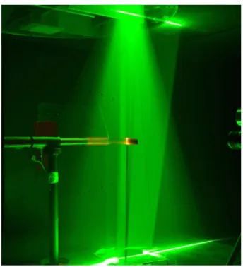
Experiments were conducted in the wind tunnel of Arts et Métiers-ParisTech, see Figure 1. This wind tunnel is of a closed-circuit type and has a three-blade axial fan with a rotor diameter of 3 m. The fan is driven by a frequency-controlled asynchronous motor with a power of 120 kW. Flow is decelerated in a settling chamber behind the fan, of which the chamber is equipped with honeycomb strengtheners and wire mesh in order to smoothen the flow. The tunnel nozzle accelerates the wind from settling chamber to test section up to 40 m/s. The nozzle has contraction ratio of 12.5, ensuring a uniform velocity profile with a turbulence ratio of less than 0.25%. The semi-guided test section has a cross-section of 1.35 m × 1.65 m and a length of 2 m. The static pressure in the test section is equal to atmospheric pressure. Hence, the upstream velocity only depends on the stagnation pressure in the settling chamber, which is measured by a pressure transducer (Furness Control FC20).
The wind tunnel is equipped with a 6-component balance. The forces are measured by means of strain gauges connected to a data acquisition system (HBM MGCPlus). The wind turbine mast is installed on the balance for rotor force measurements.
The horizontal axis wind turbine used in tests has a three-blade rotor with a diameter D = 540 mm. The tapered blade has a root chord of 40 mm and a tip chord of 30 mm. The blade is twisted and the pitch angle varies from 14° at the root to 3° at the tip. The blade section is a NACA 4418 airfoil. The nacelle diameter is only 0.08D and its length is 1.2D. Thus, the vortex wake behind the rotor is not perturbed by the mast.
Figure 1 Test bench (see online version for colours)
The rotor is mounted on a shaft that is coupled with a DC generator, with the rotor load controlled by a rheostat connected to the generator. The coupling between the rotor shaft and the generator is made by a no-contact torque transducer (HBM T20WN), which emits 360 pulses per revolution. Due to the low values of measured power, the seals of the rotor ball bearings have been removed, and grease was replaced with thin silicon oil. A fibre-optic sensor (Keyence FS20V) detects a reflective target on the shaft, from which a reference can be obtained with each blade pass. By counting the number of square signals delivered by the torque-meter, after the passage of the reference signal, it is possible to obtain the rotor’s angular position with an accuracy of 1°. Data acquisition is obtained from the data acquisition card that emits a TTL signal for triggering the PIV measurements at a desired rotor angular position.
During experiments, the upstream flow velocity V∞ is maintained at a constant 9.3 m/s, while the wind turbine rotational speed was varied from 1,600 rpm to 2,300 rpm. Thus, the Reynolds numbers calculated with blade-tip-chord and tip-peripheral velocity U, vary roughly between 90,000 and 125,000.
Data acquisition is carried out by a computer equipped with an acquisition card. At each operating point the torque
T, thrust F, rotational speed n and upstream wind velocity V∞ are measured continuously with a rate of 1 sample per second. To minimise the effect of torque fluctuations, the results are averaged over a period of five minutes before calculating the rotor power. The power coefficient Cp,
which represents the ratio of obtained power P to available power, is calculated as follows:
3 2 p P C V A ρ ∞ = (1)
where ρ is air density, and A is the rotor area. Then, the thrust coefficient is obtained as:
2 2 T F C V A ρ ∞ = (2)
The experiment permits to obtain the variation of the power coefficient Cp, see Figure 6 and the trust coefficient CT, see
Figure 7; as the tip speed ratio (TSR) varies. The TSR is calculated as the ratio between peripheral velocity and upstream wind velocity:
U TSR
V∞
= (3)
2.2 PIV investigation
The PIV system is controlled by Dantec software DynamicsStudio 2.30. The images are taken with a Nd-Yag laser at 532 nm (Litron Nano-L 200-15), with an impulse power of 200 mJ, a camera of 2,048 × 2,048 px (Dantec FlowSense 4M) equipped with the lens (Micro-Nikkor AF-S 105 mm f/2.8G IF-ED), a frame-grabber card and a synchronisation system for synchronising image sensor and laser flashes with the blade angular position. The flow is seeded with micro-droplets of olive oil generated by a mist generator (Dantec 10F03). The average droplet diameter is 2–5 μm.
The study is carried out for TSRs of 4.86, 5.47, 6.08 and 7 corresponding to 1,600 rpm, 1,800 rpm, 2,000 rpm and 2,300 rpm, respectively. A series of 200 pairs of images is taken for each rotational speed. Image capture is synchronised with rotor rotation and the PIV system is triggered when the blade is positioned at the desired angular position, in this case when the reference blade is vertical. The laser sheet passes through the rotor axis and the cross-section of the tip of the reference blade. To reduce the reflections of laser radiation, the blade and the rotor casing are painted with fluorescent paint. When the blade and rotor casing are illuminated, orange light is reflected. The special narrow band filter on the lens is selected to only transmit radiation at the laser wavelength, eliminating light saturation in the image.
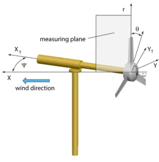
Before tests, calibration images are taken to calculate the scaling ratio and to create a spatial relationship between the camera and the blades. The PIV region of interest is shown in Figure 2. In this study, the yaw angle Ψ is zero. Taking into account the frequency of the camera (7 Hz) the images are taken once every five or six revolutions. For each pair of images, the time delay between the first and second image is set to 40 μs. This value has been experimentally established to ensure the best cross-correlation. The cross-correlation is applied to interrogation windows of 32 × 32 pixels and a 50% overlap, resulting in a spatial resolution of 3 mm.
Despite image saturation near the blades due to reflections, the velocity field is exploitable and can be used for comparison with CFD simulation. Finally, the treatment
of all PIV images has resulted in a database of instantaneous and average velocity fields for each of the four TSR. Averaged flow and vorticity fields for azimuth position of 0° are presented in Figures 8 and 9.
Figure 2 PIV plane of measurement (see online version for colours)
3 Numerical model
3.1 Hybrid modelling
The flow around a wind turbine is governed by the 3D incompressible Navier-Stokes equations:
( )
V V V f 1grad p V t ρ ν ∂ ∇ + = − + Δ ∂ G G G G G (4) Here, the velocity field is obtained as a solution of theboundary value problem, with the no-slip boundary condition V = 0 on the wind turbine surfaces. However, a high mesh density is needed in the vicinity of the rotor blades to obtain an accurate solution, for resolution of the blade section boundary layer. Usually, the number of nodes used for modelling the rotor is equivalent to those used for the wake. To facilitate the wake modelling and to reduce the computational cost, the hybrid model was developed (Vermeer et al., 2003). In this modelling, the real rotor geometry is replaced by source terms that account for equivalent forces. Depending on the distribution of the source terms, there exist three types of hybrid models: AD, AL and AS.
In the case of wind turbine, the boundary value problem is solved for Navier-Stokes equations using the appropriate no-slip boundary condition at the surfaces, corresponding to walls. As a result, the obtained velocity field depends directly on the blade section’s geometry. However, in the case of hybrid modelling, there are no walls within the fluid domain; the blades are replaced by the volume or surface forces. In this case, the boundary conditions are applied
only on external surfaces of domain. A priori, the blade forces are unknown, and their values are obtained iteratively during the calculation using the blade element method. If the flow along the blade sections is close to the two-dimensional flow, the blade forces depend on inflow and the blade section’s aerodynamic properties. This assumption is justified for most blade sections except at the root and at the tip, where the flow is 3D.
3.2 AS model
In the AS model, the rotor geometry is simplified and the blades are replaced by surfaces with a boundary condition of the ‘pressure discontinuity’ type. The surface forces, which replace the rigid blade wall, are calculated from inflow and airfoil performance. In this case, the grid density depends only on pressure distribution gradient. Hence, the number of computation nodes is significantly reduced, as there is no need to model the boundary layer.
It must be noted that the AS model can represent only the normal forces acting on the blade section. Usually, the blade section tangential forces are lower than normal forces and can be neglected. However, at some angles of attack, these forces play a significant role. In order to improve the force representation, tangential forces are imposed as body forces in a thin layer near the surface of pressure discontinuity.
The actuator hybrid modelling is carried out with two modules: the first module is a CFD solver that calculates the flow in the simulation domain with the appropriate boundary condition, and the second extracts inflow and uses blade element theory to determine pressure discontinuity. The solution is carried out iteratively, exchanging data between the blade element and CFD modules. Starting from initial conditions of the upstream flow and using the blade geometry and the airfoil data, the blade element module calculates the pressure jump distribution on the surface, which replaces the blade. The CFD module computes the flow of the velocity field, using a boundary condition of the pressure distribution previously obtained from the blade element module. The calculation stops after several iterations when the flow in the wake converges.
The calculation of pressure discontinuity is based on the blade element approach. At the blade radius r, the elementary forces acting in the normal and tangential directions on a blade element with the length dr and the chord c are: 2 1 d ( )d 2 n n F = ρW c C α r (5) and 2 1 d ( )d 2 t t F = ρW c C α r (6)
In the above formulas, the force coefficients Cn and CT can
be determined from the airfoil data CL = CL(α) and
CD = CD(α) or by means of calculation. The angle of attack
( )r ( )r ( ),r
α =ϕ −β (7)
where β(r) is the blade section pitch angle, and ϕ(r) is the flow angle between the plane of rotation and the reference relative velocity W.
It is very important to choose the right point where the reference velocity W and flow angle ϕ are to be determined. However, these flow parameters cannot be extracted directly from the inflow. The Froude-Rankine theory, applied to wind turbines, states that due to energy extraction, the flow through the rotor slows down. Betz shows that the maximum extracted energy corresponds to a velocity in the rotor plane equal to 2/3 of the upstream velocity, V∞. Therefore, the reference point must be chosen sufficiently close to the rotor. However, the flow field in the rotor plane is perturbed by the blade section, and a special approach is needed to obtain the reference velocity. The simplest way of obtaining this velocity is to calculate the mean velocity in the plane of rotation, similar to Glauert’s Blade Element-Momentum Theory (Hansen, 2007). In the case of yaw, however, the results become incorrect. In this study, a method similar to that proposed by (Shen et al., 2009) is adopted. The method is based on assumption that the inflow is the sum of the upstream velocity, the local induced flow (created by the presence of the blade section), and an AD (which extracts kinetic energy and decelerates the flow passing through the rotor). As a result, the reference point can be located sufficiently close to the rotor if the blade perturbations are excluded from velocity field obtained by CFD solver, by subtraction of the blade induced velocity. The simplest way to calculate this induced velocity is to represent the airfoil by a point vortex, vortex sheet, or airfoil vorticity of equal circulation.
4 Numerical model
The studied wind turbine model is similar to that tested in the wind tunnel. The choice of studying this wind turbine provides a comparison between the results of wake simulation and experimental data. If the large wind turbine is studied, like in MEXICO project (Schepers and Snel 2007), only a limited comparison of flow field will be available. In fact, the PIV measurements are constrained by the laser power and camera resolution to limited areas.
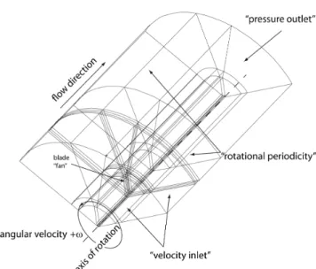
To facilitate the calculation, the simulation domain represents a cylindrical sector with a blade period, and is therefore equal to one third of the domain, for a three-blade rotor. The domain, with a diameter of 5D and a length of 15D, is divided into four parts (see Figure 3). The first part, upstream of the rotor, has a length of 5D and where the grid approaching the rotor becomes dense.
The second part, containing the pressure discontinuity surface, consists of a fine mesh. This high grid density is necessary for a good representation of the velocity profile behind the rotor, which determines the initial development of the wake. In order to describe the distribution of pressure discontinuity, the surface replacing the blade is divided into 80 intervals in chord-wise direction and into 100 intervals
spanwise. The mesh is finer near leading edge, blade tip, and root because the pressure gradient in these areas is most important. The initial cell layer height is equal to 0.02 the chord length, and cell growth ratio is 1.05, which is needed to distribute precisely the body forces acting in the chord-wise direction.
Figure 3 Simulation domain
The third part of simulation domain has a length of 1D, and also has a fine mesh. This part contains most of the length of near wake, and the high grid density is needed in order to represent the vortices, trailing from the tips of the blades. In this part, the cell size represents 0.005D. The fourth and last part of the volume is similar to the first, with a decreasing mesh density away from the rotor. This part represents the development of the far wake.
In radial direction, each of four parts is divided into three annuli: internal, intermediate, and external. The internal annulus has a diameter of 1D and contains most of the wake. The intermediate annulus has a diameter of 1.4D and contains the tip vortices and wake shear layer. Here, the cells are cube-shaped in order to avoid grid-oriented numerical diffusion of the vortices. The internal and the intermediate annuli have a denser grid as compared to the external annulus due to wake development there. The external volume is needed to represent free stream velocity not perturbed by rotor.
The total number of cells of this multi-block structured grid has been limited to 13 million, in order to perform the simulation on a single multiprocessor machine. Thus, in case of wind farms, where simulation is performed on PC’s, one computer would be able to calculate the flow around one wind turbine.
All simulations are carried out using CFD solver ANSYS
Fluent 12.1. The simulations are performed with an
upstream velocity of 9.3 m/s and turbulence of 0.3%, corresponding to wind tunnel conditions. To calculate the performance of the wind turbine being studied, only the angular velocity is varied, with upstream velocity and turbulence kept constant.
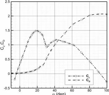
A ‘velocity inlet’ boundary condition is applied on the inlet and on the peripheral surfaces of the simulation domain. The ‘rotational periodicity’ boundary condition is applied on the lateral surfaces of the simulation domain. On the surface, which represents the blade, the ‘fan’ boundary condition is applied. In this study, the lift and drag coefficients are calculated from the inflow over the blade section, from the blade geometry, and from the experimental performance of a NACA 4418 airfoil, obtained by Ostowari and Naik (1985), see Figure 4. Because the experimental data does not include the pressure distribution, the lift force is distributed using a simplified pressure distribution. See Dobrevet al. (2007).
Figure 4 NACA 4418 aerodynamic performance
In this study the reference velocity is calculated at a distance of one chord upstream of the blade section, see Figure 5. At this distance, the perturbation due to the blade is important. To take into account this perturbation, the velocity induced by the blade section is subtracted from the velocity calculated by the CFD solver. This induced velocity is assumed to be equal to that induced by an airfoil in potential flow, which has a vorticity distribution equivalent to the pressure distribution over the blade (Figure 5).
To obtain this pressure distribution, for each node of the pressure discontinuity surface, velocity, the local angle of attack α, the distance s/c to the leading edge, and the relative radius r/R must be calculated.
To take into account the angular rotation of the rotor, a multi-reference frame (MRF) is used. The computation is performed using detached eddy simulation k-ω (DES k-ω) and bounded with a central differencing scheme applied to discretise the momentum equation. The time step varies depending on rotational speed: for a rotational speed of 1800 rpm the time step is 3.125 10–4 s which corresponds to an angular step of 3°.
Calculations are carried out iteratively and after numerous iterations, according to the number of the nodes and the value of the residuals required for convergence. The
computed rotor power reaches a constant value quickly, usually after 500 iterations (difference less than 0.05%). However, more than 3,000 iterations are required to obtain sufficient wake development. This number of iterations corresponds to 25 rotations of the rotor, but it is not possible to formulate an absolute criterion on wake convergence. In practice, the wake is characterised by important unsteadiness, vortex wandering, and depends on wind turbine operating point.
Figure 5 Hybrid model calculation (see online version for colours)
5 Numerical and experimental results
5.1 Power and thrust
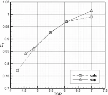
The comparison of wind turbine performance obtained experimentally and numerically with the AS scheme is presented in Figure 6 for the coefficient of power and in Figure 7 for the coefficient of thrust. Curves are denoted with ‘calc’. for simulation results, and ‘exp’. for experiment results.
The simulation results for the power are satisfactory for a TSR equal to or greater than the optimum TSR (for which the Cp is a maximum).
The accuracy of the thrust and power coefficients calculated by means of this method is dependent on specific airfoil aerodynamics, as with any method based on blade element theory. It is sometimes difficult to provide the experimental data for similar Reynolds number as in the studied case; for large Reynolds numbers, the airfoil performance does not vary significantly. For small Reynolds numbers, such as those experienced in this study, the stall angle and maximum lift coefficient vary significantly with Reynolds number (Ostowari and Naik, 1985). It must be noted also that the airfoil data in the post-stall region shows some discrepancies from measurement uncertainties (McAlister et al., 1978). Therefore, for high angles of attack, lift and drag uncertainties are non-trivial. Wind
turbines operate at high angles of attack with low tip-speed ratios, resulting in higher discrepancies.
Figure 6 Variation of coefficient of power with TSR
Figure 7 Variation of coefficient of thrust with TSR
It should be noted, however, that the uncertainty in airfoil data has more of an influence on the power coefficient than on the thrust coefficient. This is due to the fact that the blade element tangential force coefficient Cy, see Figure 8,
responsible for creating torque, is a result of the subtraction of the circumferential components of lift and drag.
sin cos
y L D
C =C ϕ−C ϕ (8)
For high angles of attack, lift and drag forces are comparable; it is possible for this difference to reach the same order of magnitude as the error itself. Subsequently, any error in the data will highly influence the value of the resultant. However, this error will have a lower effect on the overall accuracy of the resulting thrust force, as the blade
element axial force coefficient Cx is calculated from the
addition of the lift and drag components sin cos
x L D
C =C ϕ+C ϕ (9)
Figure 8 Blade section forces
Another reason for this discrepancy, which occurs for low TSR, is due to fact that flow occurs in all three dimensions and the blade-element theory becomes inexact. The experimental results (Lindenburg, 2003), show that close to the root where stall occurs, the blade-section performance becomes considerably different from those obtained for 2D airfoils.
5.2 Wake analysis
Analysis of the flow downstream of the rotor provides information on the wake’s development. Figure 9 shows the dimensionless average velocity field and Figure 10 shows the average vorticity field, depending on TSR. In these figures, the plane of exploration passes through the axis of rotation, with a vertical reference blade is vertical and flow development from left to right.
The tip vortices trailing the blades move with the fluid and as consequence are helical in shape. The plane of interest cuts through these helixes and show up as dark circles on raw PIV images. Additionally, the rotation of the vortex core separates the seeded oil droplets, reflecting the laser light.
It is easy to observe the tip vortices that govern the flow of the wake, dividing the flow into two regions: an internal zone, where the wake is restrained by the tip vortices, and an external zone corresponding to a less-perturbed free flow.
In Figure 10, tip vortices with high negative values are represented as blue circles. These negative values correspond to vortices turning in the clockwise direction, as is intended for a wind turbine. The resulting velocity from these vortices adds to the free stream velocity. As a result, flow in the external zone is accelerated (see Figure 9). Conversely, in the internal zone, these vortices induce a flow in the opposite direction of the free stream flow, and the flow is decelerated. This deceleration becomes more significant at points close to the tip vortices. Downstream of the rotor, the helical vortices decelerate the internal flow and the wake diameter gradually increases.
Figure 9 Averaged velocity field V/V∞ downstream of wind turbine rotor (see online version for colours)
Figure 10 Averaged vorticity field downstream of wind turbine rotor (see online version for colours)
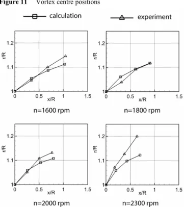
In the velocity field shown in Figure 9, the positions of the tip vortices are located where the velocity varies rapidly in the radial direction with a stronger gradient. Experimental results show that at the core centre of the vortex, velocity varies with radius from values close to zero to values two times greater than the upstream velocity. Generally, the wake simulations are satisfactory for the axial and radial positions of the tip vortices, except in the case of high rotational speed (high TSR), where the wake expansion is less than experimental measurements (see Figure 11). Figure 11 Vortex centre positions
The wake expanding behind the wind turbine depends on the vortices developed by the blade tip. These vortices induce an axial flow toward the rotor that decelerates the upstream flow. The theory of propeller shows that the induced velocity far away behind the rotor is two times greater than the induced velocity at the rotor plane. As a result, the wake expands behind the rotor and becomes constant after a distance of one or more rotor diameters. As in the numerical simulation, the intensity of the tip vortices is not preserved like in reality, then the flow is not sufficiently decelerated by induced velocity, and the wake expansion is weakened. To improve the simulation of tip vortices, grid resolution must be increased or a solver with a vorticity preserving scheme must be employed. As an increase in the number of nodes is not suitable, a solver with the appropriate scheme must be employed simultaneously.
The result for the rotor thrust coefficient in Figure 7 displays an increase in thrust with an increase in TSR. This result is confirmed by velocity field measurements, where the wake diameter increases with increasing TSR. It is therefore shown that high thrust leads to greater deceleration.
The velocity gradient obtained from simulations is less noticeable: tip vortex has a large diameter and its intensity is much lower. The difference between the experiment and the simulation is based mostly in grid coarseness; the mesh cell size is comparable with the vortex core radius. As a result, the vortex core is not well reproduced, and numerical diffusivity increases. However, due to the aforementioned computational memory limitations, cell size cannot be reduced.
The first vortex, represented on the left side of the images, is emitted from the blade previous to the reference blade with a vortex age of 120°. Here, vortex age is defined as the azimuth travel of the blade since vortex creation. Experimentation has shown that the vortex sheet trailing from the blade is tightly wound, with the highest vorticity concentrated at the tip vortex. However, in simulations the blade wake is well-defined for all TSR (Figure 10).
6 Conclusions
An improved hybrid model based on the AS is proposed in order to facilitate the simulation of wind farms. The objective of this paper has been to demonstrate the capabilities of the proposed model to represent the wake behind the rotor. The simulation domain is simplified and blades are replaced with pressure discontinuity surfaces. In the case of complete geometry simulation, the no-slip boundary condition is applied on the blades, which requires a high quality mesh for boundary layer representation. However, the appropriate modelling of the boundary layer is crucial for simulation accuracy. In the case of hybrid modelling, however, there are no walls, and blades are represented by volume and the surface forces. These forces are determined using blade section inflow and blade aerodynamic properties, reducing the overall grid density.
The AS has the same pitch angle and chord as the original blade on which the pressure discontinuity is applied. The airfoil aerodynamic characteristics are obtained from wind tunnel experiments, but the pressure distribution is unknown. In this work, a pressure discontinuity is applied, which is similar to a thin flat plate pressure distribution but without singularity at the leading edge.
The proposed model is tested in the case of flow around a horizontal-axis wind turbine model for four TSRs. The results of simulations are compared with the results of experiments carried out in the wind tunnel. The comparison shows the efficiency of the proposed AS model to reproduce the rotor mechanical power and forces, but for low TSRs, some discrepancy with experimental results is observed. In the case of low TSRs, the angle of attack increases along the blade span and the flow becomes detached and highly three-dimensional. In this case the blade element method, used to determine the aerodynamic forces, is not adequate alone.
Generally, the wake simulations are satisfactory for the axial and radial positions of the tip vortices, except in the case of a high TSR, where the wake expansion is less than found experimentally. It is believed that the discrepancy is due to reduced tip vortex intensity. Therefore an appropriate scheme of calculation that preserves vorticity is required. Finally, it must be noted that the simulation cannot reproduce the recirculation zone behind the rotor.
References
Boyd, D., Barnwell, R. and Gorton, S. (2000) ‘A computational model for rotor-fuselage interactional aerodynamics’, AIAA paper 2000-0256.
Dobrev, I. and Massouh, F. (2005) ‘Etude d’un modèle hybride pour représenter l’écoulement à travers un rotor éolien’, 17 Congrès Français de Mécanique, 29 August–2 September, Troyes, France.
Dobrev, I., Massouh, F. and Rapin, M. (2007) ‘Actuator surface hybrid model’, Journal of Physics: Conference Series, Vol. 75, Paper No. 012019, 7pp.
Hand M. et al. (2001) ‘Unsteady aerodynamics experiment phase VI: wind tunnel test configurations and available data campaigns’, TR NREL/TP-500-29955.
Hansen, M. (2007) Aerodynamics of Wind Turbines, 2nd ed., Earthscan, London.
Krogstad, P-A. and Eriksen, P. (2013) ‘‘Blind test’ calculations of the performance and wake development for a model wind turbine’, Renewable Energy, February, Vol. 50, pp.325–333. Lindenburg, C. (2003) ‘Investigation into rotor blade
aerodynamics’, ECN Report: ECN-C-03-025.
McAlister, K., Carr, L. and McCroskey, W. (1978) ‘Dynamic stall experiments on the NACA 0012 airfoil’, NASA.TP-1100. Mikkelsen, R. (2003) Actuator Disc Methods Applied to Wind
Turbines, PhD thesis, Technical University of Denmark.
Ostowari, C. and Naik, D. (1985) ‘Post stall studies of untwisted varying aspect ratio blades with NACA 44XX series airfoil sections – Part II’, Wind Engineering, Vol. 9, No. 3, pp.149–164.
Sanderse, B., van der Pijl, S.P. and Koren, B. (2011) ‘Review of computational fluid dynamics for wind turbine wake aerodynamics’, Wind Energy, Vol. 14, No. 7, pp.799–819. Schepers, J.G. and Snel, H. (2007) ‘Model experiments in
controlled conditions’, ECN Report: ECN-E-07-042.
Shen, W., Zhang, J. and Sørensen, J. (2009) ‘The actuator surface model: a new Navier-Stokes based model for rotor computations’, Journal of Solar Energy Engineering, Vol. 131, No. 1, Paper No. 011002, 9pp.
Sørensen, J. and Shen, W. (2002) ‘Numerical modelling of wind turbine wakes’, Journal of Fluids Engineering, Vol. 124, No. 2, pp.393–399.
Vermeer, L.J., Sorensen, J.N. and Crespo, A. (2003) ‘Wind turbine wake aerodynamics’, Progress in Aerospace Sciences, Vol. 39, Nos. 6–7, pp.467–510.
Watters, C.S., Breton, S.P. and Masson, C. (2007) ‘Recent advances in modelling of wind turbine wake vortical structure using a differential actuator disk theory’, Journal of Physics:
Conference Series, Vol. 75, Paper No. 012037, 11pp.
Watters, C.S., Breton, S.P. and Masson, C. (2010) ‘Application of the actuator surface concept to wind turbine rotor aerodynamics’, Wind Energy, Vol. 13, No. 5, pp.433–447.
Nomenclature
A Rotor swept area
CD Drag coefficient
CL Lift coefficient
Cn Normal force coefficient
CT Tangential force coefficient
Cx Blade element axial force coefficient
Cy Blade element tangential force coefficient
c Blade chord F Force f Source terms P Power p Pressure r Radius T Thrust t Time
TSR Tip speed ratio
U Peripheral velocity
V Velocity
W Reference relative velocity α Angle of attack β Blade angle φ Flow angle ν Kinematic viscosity ρ Density ψ Yaw angle Subscripts n Normal t Tangential ∞ Infinity