Science Arts & Métiers (SAM)
is an open access repository that collects the work of Arts et Métiers Institute of Technology researchers and makes it freely available over the web where possible.
This is an author-deposited version published in: https://sam.ensam.eu Handle ID: .http://hdl.handle.net/10985/9950
To cite this version :
Renaud PFEIFFER, Philippe LORONG, Nicolas RANC - Simulation of green wood milling with discrete element method - In: 22nd International Wood Machining Seminar (IWMS 2015), Canada, 2015-06-14 - International Wood Machining Seminar - 2015
Any correspondence concerning this service should be sent to the repository Administrator : [email protected]
SIMULATION OF GREEN WOOD MILLING WITH DISCRETE
ELEMENT METHOD
Renaud Pfeiffer1, Philippe Lorong2, Nicolas Ranc2
1 Arts et Metiers-ParisTech, LaBoMaP (EA 3633) Rue Porte de Paris, 71250 CLUNY FRANCE
2Arts et Metiers-ParisTech, PIMM (UMR CNRS 8006) 151 boulevard de l’Hôpital 75013 PARIS FRANCE
[email protected], [email protected]
ABSTRACT
During the primary transformation in wood industry, logs are faced with conical rough milling cutters commonly named slabber or canter heads. Chips produced consist of raw materials for pulp paper and particleboard industries. The process efficiency of these industries partly comes from particle size distribution. However, chips formation is greatly dependent on milling conditions and material variability.
Numerical simulation of chip fragmentation can allow some useful chip thickness prediction. In this complex situation in wood cutting, the utilization of the Discrete Element Method (DEM) is relevant.
In this method, solids are modeled with spherical discrete elements linked by cohesive bonds. However the Discrete Element Method requires a previous calibration step with simple mechanical loading. For example the nature and the mechanical properties of the cohesive bonds must be determined.
After an analysis of the different mechanical loadings in green wood milling, a complete study of green wood compression is carried out. This experimental study covers the strain rates range of 10-3 to 103 s-1 using a hydraulic compression machine and the Split Hopkinson Pressure Bar
technique.
Wood specimens at different moisture content states are compressed longitudinally. This study enables us to observe the viscoelastic and hygroscopic behaviour of wood.
The experimental and qualitative simulation results show that elastic brittle beams are not well adapted to be used in quantitative green wood milling simulations.
Keywords: DEM, Slabber, Green wood, Compression, Calibration. INTRODUCTION TO THE DISCRETE ELEMENT METHOD
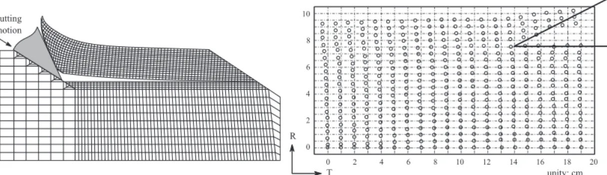
The simulation of cutting process is a long time issue. In machining, cutting simulations are widely carried out with the well-known finite element method (Figure 1). Wood is often considered as an orthotropic elastoplastic material. Strain rate effects are neglected. However this numerical method faces some issues such like tri-dimensional contacts between two meshes or fracture patterns (1-2).
Figure 1: Wood cutting simulation with the use of
Finite Element Method (From (1)).
Figure 2: Wood cutting simulation with the use of
Discrete Element Method (From (2)).
In order to avoid these problems, some authors (3-4) are using another numerical method: the Discrete Element Method (DEM). In this method, the work piece is discretised through many spheres called discrete elements (Figure 2). These elements can be linked with cohesive bonds (Figure 3) like springs, dashpots or beams.
Figure 3: Example of cohesive
bond between discrete elements (From (3)).
Figure 4: Random size and
organisation of discrete elements in a discrete domain.
Figure 5: Specified size and
organisation of discrete elements in a discrete domain.
This method, based on the fundamental principle of dynamics, is an extension of methods applied in molecular dynamics. In mechanical field it is commonly used in granular (5) or tribology (6) problems with a random disposition and size of the discrete elements (Figure 4). When applied in fibrous material cutting such like wood (2-3, Figure 2 and 3) or carbon fibres (7), the discrete elements can be placed in two different ways.
The first one consists in reproducing the organised structure of the material by structuring the discrete elements (Figure 5). In this case the mechanical properties of the cohesive bonds in the fibre direction are higher than in the two others. As the fractures occur only between discrete elements, this organisation creates an artificial fracture pattern lead by the discrete element diameter. The diameter of the sphere should be equal to the diameter of the fibres.
The second way is based on the random disposition of the elements. However the mechanical properties of the cohesive bonds depend on their inclination with the fibre axis. By this way the discrete elements are linked with many neighbours that avoid artificial motion between elements. However the size of the elements must be smaller than the fibres diameter in order to reproduce shearing between fibres.
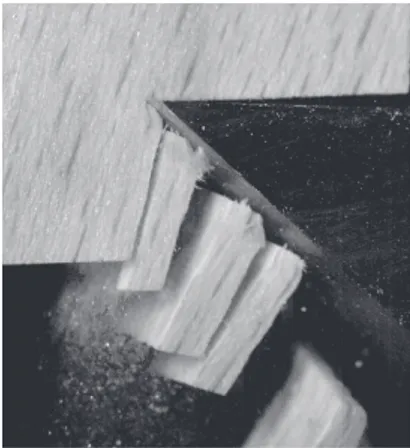
UTILISATION OF DISCRETE ELEMENT METHOD IN WOOD MACHINING The aim of this study is to simulate the chip fragementation in the wood primary transformation by slabber (or canter) heads. Previous cutting experiments on green beech were carried out (8) in order to analyse the chipping phenomena (Figure 6). Chipping films were done with a high speed camera (80000 frames per seconds).
Figure 6: Results of high speed milling experiment
on green beech (Vc = 420 m/min, h = 10 mm).
Figure 7: Qualitative DEM green wood milling
simulation with GranOO workbench (DE diameter = 1mm, h = 15 mm).
To simulate the chipping phenomena the GranOO workbench is used (9). This workbench, developed at I2M Arts et Métiers ParisTech (France), is free and open source. The parameters of the simulation are the following:
- The tool has a rigid body motion (translation at the specified cutting speed) obtained by specification of the motion for each discrete elements. No cohesive bond links the discrete elements. The diameter of the discrete elements is about 2 mm.
- The workpiece, composed of discrete elements with a diameter of 1 mm, is fixed at the top and at the left (Figure 7). The elements are linked with brittle elastic cylindrical beams. The Young modulus and the failure stress of beams in the fibre direction (here vertical) are ten times higher than in the transverse directions (here horizontal).
- Coulomb friction model is applied at the interface between the tool and the wood.
As all the computational steps are not yet parallelised, this 13500 discrete elements simulation cost ten processor hours.
The results in Figure 7 show that this method reproduces well the chipping phenomena with variable chip thickness, regular fractures under the cutting face and tri-dimensional motions of the fibres near the cutting edge. However the brittle elastic beams with a unique failure criterion for all mechanical loading is not well adapted for cutting. Multiple failure criterions depending on the load must be implemented.
In order to obtain quantitative results, the mechanical behaviour of wood in tension, compression, shearing at high strain rates (higher than 1000/s) must be implemented in the code. Moreover as the DEM is not based on the continuous media mechanics, a calibration step is required (10). This calibration step is essential when the discrete elements are randomly placed. For aligned elements, elastic calibration consists in modifying the material stiffness by the number of elastic bonds in series and parallel.
LONGITUDINAL CRUSHING BEHAVIOUR OF WOOD
In green wood milling, free water is ejected. In compression at the cutting edge, the portion of water in the lumen must drive the mechanical behaviour of green wood. Only few studies were carried out on green wood compression. Some databases (11) gather the mechanical characteristics of green and dry wood at low strain rates. At high strain rates Widehammar (12) studied the behaviour of wood at different strain rates and moisture content for spruce.
Material and methods
Longitudinal crushing experiments on wood are carried out on two experimental devices. The first one is a servo hydraulic tensile-compression machine MTS with a load cell of 100 kN. Contrary to the ASTM D143 (13) and NF B51-017 (14) norms the testing machine is not equipped with a rotating plate but with an alignment fixture (MTS 609). A constant strain rate of 10-3, 10-2, 10-1, 1
or 10 s-1 is applied during all the experiments. Force and hydraulic jack displacement are
measured.
As at a strain rate of 10 s-1the displacement error reaches 20%, Split Hopkinson Pressure Bars are
used to obtain quantitative results at higher strain rates. This experimental device is based on wave propagations and the specimen mechanical impedance must be adapted to the bars impedances (15). That is why 2 m long and 38.2 mm diameter magnesium alloy Mg ZK60 T5 bars are used. The gas gun is filled with compressed air at a pressure of 4 bars, which represents a mean strain rate of 550 s-1. The three-wave technic (15) is used to obtain stress strain curves.
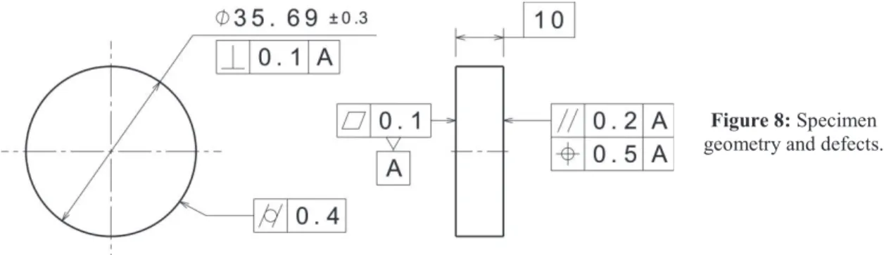
The specimen geometry is represented on Figure 8. Its section is set to 1000 mm2. The
geometrical defects are due to the machining process (turning, sawing and sanding with a specific apparatus).
Figure 8: Specimen
geometry and defects.
Fresh green beech is chosen for the crushing experiments. The same species was used for the previous milling experiments. Three moisture content levels are chosen by placing specimen in different environments. To keep the initial moisture content (55 %), one part of the specimen is wrapped with plastic and put into a fridge. To increase the moisture content (95 %) another part is sunk into water. The last part is dried up to 20 %. The moisture contents are computed by the double weight technique. At each strain rate and moisture content the crushing experiments are repeated 30 times.
Results
The obtained strain stress curves can be found in Figure 9. At each moisture content wood exhibits a viscous behaviour with an augmentation of the stresses with the strain rate. Under a strain rate of 10 s-1, longitudinal crushing response of wood decreases when moisture content
increases. At 550 s-1, the crushing strength augments with moisture content above the fibre
saturation point.
From these curves, some specific mechanical properties are studied with respect to Adalian “Wood model” (16). A particular attention is paid to initial stiffness, proportional limit and the associated strain, crushing strength and its associated strain, the specific absorbed energy and the plateau stress and stiffness.
Figure 9: Crushing mechanical response of beech in longitudinal direction function of strain rates and
moisture content.
The initial stiffness is computed by linear interpolation around the point where the derivation of the stress with respect to the time is minimal. An R2 criterion is fixed (0.99). The proportional
limit and its strain represent the end of the linear interpolation.
The crushing strength is calculated at the point where the derivative of the stress with respect to the time is null.
As far as the plateau stress is concerned, we use the mean stress value between 5 and 10 % of strain. The plateau stiffness corresponds to a linear interpolation between 5 and 10 % of strain. Finally, the specific absorbed energy is computed by integration of the stress up to 10 % of strain. For all these mechanical properties, a variance analysis (ANOVA) is performed. The chosen model is the following:
S ti ff n es s ( G P a ) P rop or ti on a l li m it ( M P a) S tr ai n at p rop or ti on a l li m it ( %) C ru sh in g st r e n gt h ( M P a ) S tr ai n at c r u sh in g st r e n gt h ( %) S p ec if ic ab sor b e d e n e rgy (M P a ) P lat eau s tr es s (M P a ) P lat eau s ti ff n es s (M P a ) Average value 2,89 -33,33 -2,69 -48,07 -4,87 3,52 -45,60 -28,47 Factors effects Strain rate (1/s) 0.001 -0,76 15,46 0,41 14,94 0,77 -1,00 13,76 10,33 0.01 -0,45 9,61 0,19 8,95 0,32 -0,57 7,80 14,04 0.1 -0,11 4,99 0,12 3,78 0,25 -0,20 2,77 14,10 1.0 0,20 2,95 -0,01 -1,99 -0,95 0,12 -2,42 -10,10 10.0 0,39 -0,37 -0,30 -5,01 -2,08 0,29 -7,15 32,38 550.0 0,72 -32,62 -0,42 -20,67 1,68 1,37 -14,75 -60,76 Moisture content (%) 20.0 0,93 -1,28 0,36 -6,01 0,76 0,38 -5,08 -34,12 55.0 -0,28 0,08 -0,14 1,31 0,02 -0,09 0,25 28,70 95.0 -0,65 1,20 -0,22 4,70 -0,79 -0,29 4,83 5,42
Interaction effect [Strain rate, Moisture content]
[0.001, 20.0] -0,07 -0,09 -0,04 -0,11 -0,64 0,13 -0,17 10,84 [0.001, 55.0] -0,21 1,46 -0,01 1,62 -0,20 -0,17 2,43 -24,77 [0.001, 95.0] 0,29 -1,37 0,05 -1,51 0,84 0,04 -2,25 13,93 [0.01, 20.0] -0,18 3,04 0,23 0,77 -0,14 0,07 1,44 -12,89 [0.01, 55.0] -0,04 -0,63 -0,15 -0,01 -0,26 -0,05 0,21 -25,28 [0.01, 95.0] 0,22 -2,41 -0,08 -0,76 0,39 -0,02 -1,65 38,17 [0.1, 20.0] -0,18 0,06 0,02 0,81 -0,33 0,04 1,81 -17,87 [0.1, 55.0] 0,08 -2,40 -0,10 -1,57 0,01 0,09 -1,08 -29,90 [0.1, 95.0] 0,10 2,34 0,07 0,76 0,32 -0,12 -0,73 47,77 [1.0, 20.0] -0,13 -0,06 -0,04 2,22 0,70 -0,02 2,70 -15,44 [1.0, 55.0] 0,19 -0,44 0,02 -2,41 0,78 0,17 -2,40 -15,51 [1.0, 95.0] -0,06 0,50 0,02 0,19 -1,48 -0,15 -0,30 30,94 [10.0, 20.0] -0,06 2,78 0,05 -0,15 1,08 0,11 0,67 -45,60 [10.0, 55.0] -0,10 -0,39 0,06 -0,57 -0,40 0,02 0,13 -9,68 [10.0, 95.0] 0,16 -2,39 -0,10 0,73 -0,68 -0,13 -0,80 55,29 [550.0, 20.0] 0,62 -5,73 -0,23 -3,54 -0,66 -0,32 -6,45 80,96 [550.0, 55.0] 0,09 2,40 0,18 2,94 0,06 -0,06 0,71 105,14 [550.0, 95.0] -0,71 3,33 0,04 0,60 0,60 0,38 5,74 -186,10
Statically significant at 0.01 probability level for factors and interaction
Strain rate YES YES YES YES YES YES YES YES
Moisture content YES YES YES YES YES YES YES YES
Interaction YES YES YES YES YES YES YES YES
With:
- ܻ: the observed parameter, - ܯ: the global average,
- ܧ: the effect matrix of factor A (the strain rate), - ܧ: the effect matrix of factor B (the moisture content), - ܫ: the interaction matrix of factors A and B,
- [ܣ]: the weight matrix of factor A, - [ܤ]: the weight matrix of factor B.
The results of the variance analysis are gathered in Table 2.
For all the properties studied the strain rate, the moisture content and the interaction between these two parameters are significant at the 0.01 probability level.
For example initial stiffness increases with strain rate and decreases with moisture content. However the mean value of initial stiffness is very low compared to values from literature (11). Xavier (17) made the same observation with specimens with small heights. This behaviour is due to the friction of the specimen with the compression plates.
The crushing strength increases with strain rate and decreases with moisture content. CONCLUSIONS
Discrete Element Method seems to be a relevant way to simulate chipping in green wood. However the mechanical properties implemented in the model must be calibrated with high speed crushing experiments.
The effect of strain rate, moisture content and their interaction is statically significant on longitudinal crushing experiment on beech wood.
Acknowledgements
This work was carried out in LaBoMaP and PIMM at Arts et Metiers ParisTech. We acknowledge I2M laboratory for their technical support in Discret Element Method; Robert Collet, Louis Denaud, Guillaume Pot; PIMM and LaBoMaP technicians and Morgane Pfeiffer-Laplaud for their availability and advice.
REFERENCES
1. Uhmeier A (1995) Some fundamental aspect of wood chipping. Tappi, 78(10): 79-86.
2. Holmberg S (1998) A numerical and experimental study of initial defibration of wood. Lund Institute of technology, TSVM-1010.
3. Sawada T, Ohta M (1995) Simulation of the wood cutting parallel or perpendicular to the grain by Extended Distinct Element Method. In Proceedings of the 12th International Wood Machining Seminar, pages 49 – 55.
4. Ohta M, Kawasaki B (1995) The effect of cutting speed on the surface quality in wood cutting. In Proceedings of the 12th International Wood Machining Seminar, pages 56 – 62. 5. Cundall PA, Strack ODL (1979) Discrete numerical model for granular assemblies.
Geotechnique, 29(1): 47-65.
6. Iordanoff I, Battentier A, Néauport J, Charles JL (2008) A discrete element model to investigate sub-surface damage due to surface polishing. Tribology International, 41(11): 957-964.
Proceedings of the 22ndInternational Wood Machining Seminar
June 14-17, 2015 Quebec City, Canada 64
carbone/époxy. PhD thesis, Arts et Métiers ParisTech.
8. Pfeiffer R, Collet R, Denaud LE, Fromentin G (2015) Analysis of chip formation mechanisms and modelling of slabber process. Wood Science and Technology, 49(1):777-784.
9. Granoo workbench (2015) http://www.granoo.org
10. André D, Iordanoff I, Charles JL, Néauport J (2012) Discrete element method to simulate continuous material by using the cohesive beam model. Computer methods in applied mechanics and engineering, 213: 113-125.
11. Kretschmann DE (2010) Wood Handbook. Wood as an engineering material. Chapter 5: Mechanical properties of wood. USDA Forest Products Laboratory.
12. Widehammar S (2004) Stress-strain relationships for spruce wood: Influence of strain rate, moisture content and loading direction. Experimental mechanics, 44(1): 44-48.
13. ASTM (1994) Standard test methods for small clear specimens of timber.
14. AFNOR (1988) Bois – Traction parallèle aux fibres – Détermination de la résistance à la rupture en traction parallèle au fil du bois de petites éprouvettes sans défauts.
15. Gama BA, Lopatnikov SL, Gillespie JW (2004) Hopkinson bar experimental technique: a critical review. Applied mechanics reviews, 57(1-6): 223-250.
16. Adalian C, Morlier P (2002) “Wood model” for the dynamic behaviour of wood in multiaxial compression. Holz als roh-und werkstoff, 60(6): 433-439.
17. Xavier J, Jesus A, Morais J, Pinto J (2012) On the determination of the modulus of elasticity of wood by compression tests parallel to the grain. Mecânica Experimental 20: 59-65.