Publisher’s version / Version de l'éditeur: PERD/CHC Report 1-056, 2000-06-12
READ THESE TERMS AND CONDITIONS CAREFULLY BEFORE USING THIS WEBSITE.
https://nrc-publications.canada.ca/eng/copyright
Vous avez des questions? Nous pouvons vous aider. Pour communiquer directement avec un auteur, consultez la première page de la revue dans laquelle son article a été publié afin de trouver ses coordonnées. Si vous n’arrivez pas à les repérer, communiquez avec nous à [email protected].
Questions? Contact the NRC Publications Archive team at
[email protected]. If you wish to email the authors directly, please see the first page of the publication for their contact information.
For the publisher’s version, please access the DOI link below./ Pour consulter la version de l’éditeur, utilisez le lien DOI ci-dessous.
https://doi.org/10.4224/12341009
Access and use of this website and the material on it are subject to the Terms and Conditions set forth at
Factors Affecting Ice Loads on Wide Structures Morse, B.
https://publications-cnrc.canada.ca/fra/droits
L’accès à ce site Web et l’utilisation de son contenu sont assujettis aux conditions présentées dans le site LISEZ CES CONDITIONS ATTENTIVEMENT AVANT D’UTILISER CE SITE WEB.
NRC Publications Record / Notice d'Archives des publications de CNRC:
https://nrc-publications.canada.ca/eng/view/object/?id=5c703f84-72d3-4fc9-a249-44e54391e090 https://publications-cnrc.canada.ca/fra/voir/objet/?id=5c703f84-72d3-4fc9-a249-44e54391e090
ICE/STRUCTURE INTERACTION
Factors Affecting Ice Loads on Wide Structures
An analysis of ice loads on the St. Lawrence River ice booms from
1994 to 2000
PERD/CHC Report 10-56
June 12, 2000
Brian Morse Université Laval
Table of contents 1 Acknowledgements... 5 2 Disclaimer... 6 3 Introduction... 7 4 The issues ... 10 5 Scope of work ... 10 6 Environmental Forces... 12 6.1 Theoretical background... 12
6.2 Environmental ice loads under laterally confined conditions ... 12
6.3 Environmental ice loads under laterally unconfined conditions ... 17
6.4 Environmental loads for St. Lawrence River booms... 20
6.4.1 Water currents ... 20
6.5 Wind conditions... 21
6.6 Ice thickness ... 21
6.7 Force calculation ... 26
6.7.1 Michel's equation ... 26
6.7.2 Comparison of estimated forces ... 27
7 Analysis of Ice/Structure interaction... 28
7.1 Analysis of load retaining capacity ... 28
7.1.1 Anchor cables ... 28
7.1.2 Section cables... 28
7.1.3 Connecting chains ... 29
7.1.4 Pontoons... 30
7.1.5 For pontoon equilibrium: ... 30
7.1.6 For section cable equilibrium: ... 30
7.1.7 From geometric relationships:... 31
7.1.8 For the ice sheet: ... 31
7.1.9 For the whole thing:... 31
7.1.10 Summary... 34
7.1.11 Limitations regarding the ice/structure interface... 35
7.2 Analysis of flexural resistance ... 36
8 Estimating ultimate applied loads: Methodology... 40
8.1 From elements that occasionally break... 40
8.1.1 Anchor cables ... 40
8.1.2 Section cables... 41
8.1.3 Chains... 42
8.2 From mechanical means... 42
8.3 From load cells... 50
8.4 Load measurement methodology: Summary & Conclusion ... 55
9 Load dynamics... 55
9.1 Section to section loading dynamics ... 58
9.2 Spectral analysis ... 62
9.3 Seasonal loading... 63
9.4 Lateral force dynamics ... 66
10.1 Spatial-temporal distribution at Yamachiche... 68 10.2 Statistical analysis ... 70 10.2.1 Statistical distribution ... 80 10.2.2 Summary... 81 11 Findings ... 82 11.1 Peak loads... 82 11.2 Spatial-temporal analysis... 83 11.3 Loading dynamics... 84 12 Conclusions ... 84 13 References ... 86
14 Annex 1. Section and anchor cables of the St. Lawrence river booms ... 94
15 Annex 2. Measured Anchor Loads on St. Lawrence River Ice booms at Yamachiche, Lavaltrie and Lanoraie 1994-2000... 98
List of Tables
6.1 Measured water drag coefficients……….……… 15
6.2 Average and maximal currents at Lanoraie and Lavaltrie.……… 20
6.3 Average surface currents at Lavaltrie boom location…….……… 21
6.4 Maximum and average ice thickness for Lac St-Pierre……… 22
6.5 Average forces estimated by Abdelnour et al. equation……… 27
6.6 Maximal forces estimated by different equations……… 27
8.1 Comparison of ultimate annual loads from mechanical means and load cells 49 9.1 Maximum load cell anchor cable load by season………...……… 64
10.1 Maximum annual line loads measured on St.Lawrence boom anchor cables 71
List of Figures
3.1 Wakefield ice boom……… 73.2 Three-dimensional view of a multi-span ice boom……… 8
5.1 Location of St. Lawrence River Ice booms…………..……….… 11
6.1 General stress distribution in an ice cover……….……… 14
6.2 Ice accumulation in front of the boom……….… 18
6.3 Wind speed 1994/1995……… 23
6.4 Measured ice thickness on Lac St. Pierre ……… 24
6.5 Predicted ice thickness on Lac St-Pierre……… 25
7.1 Definition sketch for pontoon force balance equations.……… 30
7.2 Calculated line load capacity……… 32
7.3 Calculated chain angle……….………. 32
7.4 Rotation angle of the pontoon………..……… 33
7.5 Calculated tensile force in chains……….……… 34
7.6 Boom retention capacity and internal strength of ice……… 38
7.7 Ratio of ice boom line load capacity to internal resistance of the ice…… 39
8.1 Cable clamp twisting a section cable………..……… 41
8.2 Small cage deployed on chain between pontoon and section cable 43 8.3 Load cell and ball sandwich (for chains)……….……… 44
8.4 Typical load cell deployment at Yamachiche boom…..……… 45
8.5 Load cells ready for deployment………..……… 46
8.6 Penetration of ball bearings into aluminium plates……… 47
8.7 Press used to calibrate mechanical measurements of loads……… 48
8.8 Measured loads from ball bearing sandwich and load cells……… 49
8.9 Maximum two-minute and hourly anchor loads……… 51
8.10 Loads at junction plate no.4 of the Yamachiche boom……… 53
8.11 Loads on anchor cable at the Yamachiche ice boom……… 54
9.1 Loads on anchor cable : Comparison of instantaneous and daily maximum values section cables……….……… 56
9.3 The 2.5 km wide Yamachiche boom……… 60
9.4 Force on anchor cable no 4: Yamachiche section cable……… 61
9.5 Spectral analysis at Yamachiche, winter 1999-2000……… 62
9.6 Spectral analysis at Yamachiche-alternative view……… 63
9.7 Peak load cell seasonal loads: Yamachiche anchor cables……… 65
9.8 Force imbalance in section cables and displacement of a junction plate. 67 9.9 Shift in junction plate to compensate eccentric loading in section plate… 68 10.1 Spatial-temporal distribution of maximum anchor cable loads at Yamachiche boom……… 69
10.2 Situating Measured line load peak annual data within a generic plot of different statistical distributions………..……… 72
10.3 Peak annual load plotted against the normal distribution……… 73
10.4 Peak annual load plotted against the log-normal distribution……… 74
10.5 Graph not available of Pearson III……… 75
10.6 Peak annual load plotted against the LPIII distribution……… 75
10.7 Peak annual load plotted against the Gumbel distribution………..… 76
10.8 Peak annual load plotted against the log-normal distribution………. 77
10.9 Peak annual load plotted against all distributions….……… 78
1 Acknowledgements
The report was funded by the Canadian Federal Government's Panel on Energy Research and Development (Ice/Structure Interaction programme).
On behalf of PERD, Dr. Garry Timco of the Canadian Hydraulics Centre (CHC) of the National Research Council managed the project and provided moral support.
Dr. Samir Gharbi, Université Laval, assembled the data and wrote Chapter 6 (analysis of environmental forces).
Libo Sun typed the Reference list.
Gervais Bouchard of the Canadian Coast Guard (Laurentian Region) supported CCG-RL's collaboration in the study.
Stéphane Dumont, CCG-RL retrieved and provided all the force data. He also looked after the calibration of the load cells and wrote a historical account of the booms' evolution. He also provided advice and comments (but has not yet seen this report). He is the engineer responsible for the booms and the technical group looking after the data and the boom maintenance and improvement. With the principal author and others, he helped developed the data acquisition systems.
Marc Choquette, CCG-RL helped design, improve and deploy the booms. He also provided many insights and comments. He is responsible for most photographs shown in the report. He oversees the data acquisition and boom maintenance. Marc also provided almost all the photographs and sketches contained in this report.
Marc Savard, CCG-RL also helped improve and deploy the booms. He also is responsible for the maintenance of the data acquisition systems and data retrieval. He provided access to all the environmental data and videos of the booms.
We note that a number of partners and clients participated in the boom's design and evolution. Particularly, CHC, Fleet Technology, Le Groupe Conseil LaSalle, INRS-Eau and Donald Carter.
We thank Ed Stander for his review.
We are very grateful to all who have helped (and will, no doubt, continue to help) in this project.
2 Disclaimer
This report was prepared to the best of our knowledge using the best information we had at hand. Nevertheless there may be some errors or omissions. In this case, the principal author takes full responsibility.
ICE/STRUCTURE INTERACTION
Factors Affecting Ice Loads on Wide Structures
June 12, 2000
Brian Morse Université Laval
3 Introduction
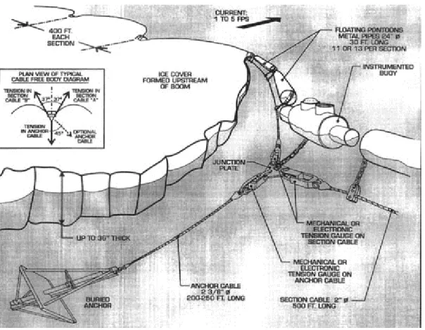
Ice booms are very wide structures intended to provoke the formation of a stable ice cover and/or retain or store ice in a certain location. They can be deployed on rivers to manage ice or at sea to contain an oil spill or to protect a fixed structure. A simple one span boom consisting of 13 cylindrical steel pontoons is shown in Figure 3.1.
More typically, as shown in the following sketch, booms are multi-span structures:
Figure 3.2. Three-dimensional view of a multi-span ice boom, Yamachiche, Québec Historically, there were many ice booms deployed in the 1960s. They were composed primarily of rectangular 14" by 22" Douglas Fir pontoons Following a major ice jam at Lac St. Pierre on the St. Lawrence River in February, 1993, the principal author designed and deployed a new boom based on cylindrical pontoons similar to the ones shown in Figures 3.1 and 3.2.
It was essential to deploy the booms quickly to prevent another ice jam in order to restore confidence in winter navigation on the river. As such, three consultants were called upon to aid in the design. Donald Carter (1995) did some analytical work. Fleet Technology (1993 & 1996) did some analytical studies and some very rudimentary physical model studies. The Canadian Hydraulics Centre (1995) performed detailed model studies of both a typical boom section and different pontoon geometries and densities. Le Groupe Conseil LaSalle (1993) performed a physical model of Lac St. Pierre to help optimise the location of the booms. INRS-Eau (1993 and 1994) complemented the work using a 2-dimensional study.
A prototype section was installed in Lac St. Pierre in 1993. The section seemed to perform very well and as such, a new boom consisting of 18 sections and 13 pontoons
per section was designed and constructed (with some assistance from Public Works Canada) in 1994. Each section was 400 ft (122 m) wide. All pontoons were 30" (61 cm) in diameter except for sections 5, 10 and 15 (see Annexe 1) which were constructed out of 76 cm pontoons. After observing the performance of the boom during the first winter, a 19 section was added on the south side (section no. 0), all 76 cm pontoons were removed and replaced with 61 cm pontoons and all sections were reduced from 13 to 11 pontoons per section. The extra section was added to promote the ice cover interaction with the artificial islands. The 76 cm booms were replaced because it was noted that these sections carried too much of the load for no good reason. Two pontoons per section were removed to avoid the pontoons hitting in to each other under wave action (during the no-ice period). (Removing 2 pontoons per section did not noticeably reduce the boom's efficiency in subsequent years).
As can be seen in Figure 3.2, the booms were deployed with load cells to measure forces in the cables. After a couple of years of deployment, a statistical analysis of the measured loads was performed primarily by the Canadian Hydraulics Centre (Cornett et al, 1997 and 1998). In addition, these booms were monitored in real time using an Integrated Ice Information System (Morse & Crookshank, 1998).
Due to the success of these booms and the enthusiasm of Fleet Technology, a number of similar booms have recently been deployed elsewhere. Locations include the Rideau River, the Ottawa River, the Pickering nuclear power station and Lake Erie. Ice booms are also proposed for the Chaudière River, to prevent jams at the Missouri / Mississippi Rivers (Tuthill and Gooch, 1998) and to control ice on the St. Maurice River (Carter, 2000).
Regarding estimated loads, Cornett et al. (1997 & 1998) demonstrated that maximum recorded loads on ice booms follow a Gumbel distribution. Timco and Cornett (1994) measured model forces required to free a boom which is frozen into an ice sheet. They also measured forces generated by ice pieces accumulating in front of booms of various sizes and shapes. Foltyn and Tuthill (1996) presented loads measured on booms deployed across North America.
Abdelnour et al (1994) and Cornett and Timco (1995) demonstrate that measured loads depend on boom geometry (size, shape and relative density) and the nature of the links between the pontoons and the cable. For Douglas Fir pontoons, Le Groupe Conseil LaSalle showed that applied forces were very dependent on the nature of the ice sheet geometry at the ice/structure interface. In the physical model studies, Cornett and Timco confirmed this finding.
Michel (1966), among others, demonstrated that loading is a function of the driving forces such as water currents and wind. In fact, he suggested that the most critical conditions could be those generated by wind.
Both the laboratory work and the statistical analysis work on prototype data done at the Canadian Hydraulics Centre (CHC) showed that applied loads are a stochastic process.
4 The
issues
There are principally two issues regarding these booms. First, despite all the research conducted to date, there is still no definitive document that clearly describes and quantifies the ice/structure interaction for these booms. Second, there is no document that describes the performance of the booms in view of their design.
5 Scope of work
In this report, we would like to address these two issues.
First, we estimate ice/structure loading based on three theoretical approaches:
1. We describe different formulas to calculate the environmental forces that the ice cover can apply on the structure. This section is based on very traditional formula and has been applied to calculate potentially extreme loading conditions. It does not take into account an alternative expression developed by Carter (2000) because at the time of writing, we have not yet received his permission to do so. It does not use Shen's (2000) new material aggregate ice model for ice accumulations. It does not use historically recorded wind speed and flow rate data to calculate historical estimates of the ice loading. This data was received to late from the Canadian Coast Guard to include it in this report.
2. The second component of our analysis is an attempt to estimate the maximum applied force that an ice sheet can deliver under bucking and flexural modes of failure. We note that Timco and Cornett's study indicates that for booms similar to the ones examined here (61 cm pontoons), the mode of failure is flexural.
3. The third component of the theoretical analysis is a little more detailed. Using a simple perpendicular-faced ice sheet, based on an analysis of the boom geometry, we develop equations describing the boom's capability to retain the ice.
Second, we present the measured data over the last five winters at three ice booms on the St. Lawrence River. The locations are, from upstream to downstream, Lavaltrie (10 sections), Lanoraie (11 sections) and Yamachiche (20 sections) (see Figure 5.1).
Figure 5.1. Location of St. Lawrence River Ice booms (Note no. of sections in 1999 is 10, 10 and 20 respectively)
We analyse the force balance equation between the forces in the section cables and the anchor cable. This is followed by an analysis of the force interplay between the tension in one section cable and its neighbour. We analyse spatial distribution of the line loads applied on the anchor cables. Using a spectral analysis we analyse the forcing frequencies and periods. We perform a statistical analysis of the maximum annual measured loads.
During the whole report, we will provide information regarding the performance of the boom, the expected loading and the associated design criteria. We hope to make a more formal summary of these findings at a latter time.
We are proud of some elements of this report. We feel that it does significantly contribute to the advancement of our understanding of the interaction between ice and wide flexible structures form a theoretical point of view, from a temporal-spatial point of view and from a statistical point of view. We also believe that its makes some inroads to explain the large variability in measured loads.
6 Environmental
Forces
6.1 Theoretical background
Many authors have studied loads generated by ice accumulations against ice booms. The most important forces result from water shear on the underside of the ice cover, the wind stress on the ice cover surface and the down slope component of the gravity forces on ice accumulation. Additional forces include ice impact forces, hydrodynamic forces on the frontal edge of the ice accumulation and forces resulting from vessel passing close to the boom (Foltyn and Tuthill, 1996).
The total force on an ice boom ca be expressed as the sum of the following forces:
v w i i a w F W P P F F P = ± + + + + (6.1) Where:
Fw : water shear on the underside of the ice accumulation Fa : wind drag force on the ice cover
Wi : down-slope component of the gravity force on the ice accumulation Pi : force resulting from ice impact
Pw : hydrodynamic force on the frontal edge of the ice accumulation Fv : force resulting from vessel passage
Latyshenkoff (1946) showed experimentally that as the length of the ice accumulation behind the boom increased, the load exerted by the ice did not build up indefinitely but reached some maximum value. One of the most common problems of the determination of the forces exerted by an ice field is estimating the length or area of the ice cover that contributes to the ice load on the boom. In the literature, there are essentially two approaches to determine the contributing area pushing against an ice boom. The first, normally referred to as Caquot's theory uses the grain in a silo analogy. Ice is considered to be a granular material confined within two parallel side walls. The second approach is used where confinement is unlimited. In this case, the ice accumulation takes on the form of a triangle. The area behind the boom is dependent on the boom width and the apex angle of the triangle.
6.2 Environmental ice loads under laterally confined conditions
In 1959, Beccat and Michel (1959) applied Janseen's grain elevator theory. They concluded :
- a part of the ice load is applied to the river banks through the arching of inter ice floes - the maximum force on ice booms is achieved when the reaction of the banks is equal to any additional incremental load added upstream on the ice accumulation.
- parabolic arches corresponding to the principle directions of the internal inter ice floe stresses make up the final equilibrium load system.
The stress distribution in an ice accumulation is similar to the one of the two-dimensional grain elevator with a top load. The total stress is made up of tangential force (τ) and force exerted at the frontal edge (p0) (see Figure 6.1)
The total force exerted on an arch at a distance x from the edge is given by − − + − = B x B B x B p F ξ ξ τ ξ 1 exp 2 exp 0 (6.2) Where: B: channel width
ξ : coefficient of lateral confinement which depends on angle friction of the ice on the shore (Michel, 1978).
By taking a value ξ = 0.3, Michel (1978) obtained the final formulas:
B p B F B x F F τ α τ α 3 . 3 1 3 . 3 3 . 0 exp 1 0 2 − = = − − = ∞ ∞ (6.3)
Figure 6.1 : General stress distribution in an ice cover (Michel, 1978)
The tangential force is calculated as follows:
τ = τw + τa + η (6.4) Where
τw : water tangential stress τa : wind tangential stress
φ τ P x Sect. 1 B o σ σ σ σ α α σ σ r y x n1 n1 n1 σn2 + ²σn1 τ Y o h h Y Y ' V V o o L Plan Section
η: longitudinal component of the weight of the ice accumulation 2 V CD w ρ τ = (6.5) where V is the water velocity (m/s), ρ is the mass density of water (1000 kg/m3) and CD is the drag coefficient of water.
Suggested values of CDare presented in the following table.
Table 6.1: Measured water drag coefficients (based on Carter, 1995)*-
Author CD (1m)
X 10-3 Johannessen (1970) very rough 26.6 rough 12.8 smooth 13.4 Untersteiner & Badgley (1965) 10.5
McPhee (1975) 3.4 Campbell (1965) 12.0 Hunkins(1966) 7.8 Michel (1978) 3.9 Carter (1995) 41.3 2 U CDair air a ρ τ = (6.6) where U is the wind velocity (m/s), ρair is the mass density of air (1.293 kg/m3 at 0oC) and CDair is the drag coefficient of flowing air over the ice cover.
The range of values of CDair reported by Michel (1978) is 1.3X10⁻³ to 4.4X10⁻³. Foltyn
and Tuthill (1996) gave a range 1.7X10⁻³ – 2.2X10⁻³.
The gravity stress is given by : hS
eγice
where γice is the specific weight of ice and e is the porosity (0.3), it is found
hS 4410 =
η (6.8) The hydrodynamic force on the frontal edge (p0) is given by the momentum theory. This force is generally neglected in the computation of forces exerted by ice on structures. Michel (1978) estimated the maximum hydraulic thrust and thrust caused by wind by using the following assumptions:
the porosity of the ice accumulation = 0.3 the internal angle of friction = 30o
the wind speed = 33 m/s at standard 10 m above the ground
Michel (1966, 1978) proposed the following formula to determine the ultimate push of an ice accumulation against a boom :
Maximum hydraulic-induced load (Pw):
Pw = 0.016 h2 B (kN) (6.9)
where h is the ice thickness (m) and B is the width (m). Maximum wind-induced load (Pa):
Pa= 0.0176 B2 (kN) (6.10)
However, since the ice accumulation cannot thicken by an amount greater than the river depth (H), (the river bottom would then take a great part of the load), there is a limitation given by
B h Pa 2 0 . 1 ≤ (6.11) Michel (1978) stated that the maximum possible thrust on a structure could readily be obtained from equations 6.9 to 6.11.
For a grounded ice field in a depth of water H (m), Carter (1994) deduced from Michel’s analysis that the maximum ice line load (w in kN/m) can be written as follows:
Carter (1994) used this equation to compare loads calculated by this limiting value with those measured experimentally on the Yamachiche ice booms on Lac St. Pierre. He characterised the correlation as very good given the dynamics of the loads in question.
6.3 Environmental ice loads under laterally unconfined conditions
The ice force depends on the size of the ice accumulation in front of the boom. The problem of the determination of the extent of the upstream ice accumulation has been studied since 1935 by many investigators. Latshynekoff (1946) found experimentally that the length of the ice cover attained a constant value after a length of three to four times the width of the field. The U.S. Army Corps of Engineers (1999) recommends to derive ice loads acting on the boom from an area that extends upstream an amount corresponding to five river widths. Abdelnour and al. (1993, 1996) estimated this area by evaluating the apex angle (see Figure 6.2). They state (1996) « The area covered by ice pieces retained by the boom will probably increase steadily during an event, starting with the areas in front of the individual spans (e.g. the areas labelled A1 to A8 in Figure 6.2). When two or more adjacent spans are completely filled with ice, ice pieces will then collect over a large area (e.g. areas B, C, D and E in Figure 1.2 ). The ice area will increase until it covers the total width of the boom. This will produce the highest ice forces on the boom as the ice area has reached its maximum. »
An ice cover length of three to four times longer than the width of the boom is equivalent to an apex angle ranging from 15° to 20° (Abdelnour and al. 1993). Abdelnour and al. (1991) found that an apex angle of 60° correlated well the drag force required to drive the ice cover past two different types of bridge piers at Laviolette Bridge on the St-Lawrence River. Consequently they used an apex angle of 60° in the study of Lavaltrie ice boom.
Figure 6.2: Ice accumulation in front of the boom (Abdelnour et al. (1993))
Abdelnour et al. (1995) assume that the ice accumulation in front of the boom is acted upon by wind and current forces. With their approach the currents and winds are assumed to be uniform over the area of ice cover. The wind and current forces were predicted as follows : 1 2 3 4 5 6 7 8 A1 A2 A3 A4 A5 A6 A7 A8 C B D E 400 ft
Boom span (typ.)
c D current C V A
F =ρ 2 (1.13) Fwindt =ρCDairU2Aw (1.14)
Where Fcurrent and Fwind are the current and wind drag forces respectively and Ac and Aw
are the surface areas of the ice cover acted upon the current and the wind respectively given by
( )
/2 tan 4 2 α B A Ac = w = (1.15) where α is the apex angle of the triangular ice area upstream the boom.It should be noted that the U.S. Army corps of Engineers determines the ice forces by using
2 5B A
Ac = w = (1.16)
For estimating the value of drag coefficient current, Abdelnour et al. (1995), expected a rafted ice cover. A value for CD = 0.015 was selected in the analysis of forces acting on Lac St-Pierre ice booms and CDair was taken as 0.0033. These values were found to be within the range of the loads measured by Cowper et al. (1994). It should be mentioned that these values are not constant during the winter. The ice is rough during the ice formation stage and becomes smoother when the ice consolidated (Abdelnour et al., 1995)
The line load is given by:
( )
[
1000 2 1.293 2]
2 / tan 4 C V C U B W = D + Dair α (1.17)With the values of the drag coefficients and the apex angle assumed by Abdelnour et al. (1995), equation (1.17) becomes:
[
2 2]
0043 . 0 15 433 . 0 B V U w= + (1.18)6.4
Environmental loads for St. Lawrence River booms
The wind velocity, the water currents and the ice thickness are prerequisite to the determination of loads on ice booms.
6.4.1 Water currents
For the Yamachiche boom, experimental observations were made on the northern part of Lac St-Pierre during the month of January 1995 and are reported by Carter (1995). Current profiles were made at ten locations under the ice covers. The average value of all current velocity is calculated by Carter (1995). The maximum velocity of all average values is 0,27 m/s and the mean velocity is approximately 0.16 m/s. The average current velocity in Lac S-Pierre was also obtained by Abdelnour et al. (1994) from a 2D hydrodynamic model run. The average current velocity reported is 0.35 m/s for open water current conditions.
For Lavaltrie and Lanoraie boom, an ice survey was made by the St Lawrence Ship Channel group (Department of Transport) in January, February and March 1973. The values obtained are summarised in Table 6.2.
Table 6.2 Average and maximal currents at Lanoraie and Lavaltrie Location maximal current (m/s) average currents (m/s) discharge at Sorel (m3/s) Lanoraie 0.66 0.32 11540 Lavaltrie 0.55 0.38 11334
It should be noted that these measurements were made a few metres downstream of booms. The estimated discharge in the St. Lawrence river at Sorel at that time show that the currents were measured under very in high winter discharge conditions.
Beauchemin and Pellegrin, 1969, measured the surface currents at Lavaltrie boom location. The average values are summarised in table 6.3
Table 6.3. Average surface currents at Lavaltrie boom location Survey time and date Mean surface current across full width of boom (m/s) Mean surface current across boom spans 2, 3 and 4 (m/s) 13h00 June 2, 1969 15h00 June 2, 1969 0.70 0.67 0.68 0.64
Since the Lavaltrie ice boom is located in channels parallel to the navigation channel, for the same discharge in the river, the current near the boom is expected to be lower in winter than it is in summer. Once an ice cover forms upstream of the boom, because of the increased resistance on that side of the island, relatively more of the flow will follow the main (navigation) channel.
Finally, Abdelnour et al. assumed a “design current” of 0.76 m/s for the study of Lavaltrie ice boom. The current used for the Lanoraie ice boom is slightly less than 0.70 m/s (Abdelnour et al., 1995).
6.5 Wind conditions
The wind speeds were recorded at Sorel weather station for winter 1994/1995. The wind speeds normal to the ice boom for Lavaltrie, Yamachiche and Lanoraie are shown in Figure 6.3 (Abdelnour et al., 1995). This figure indicates that the normal wind speeds are almost identical for all three booms. So, it can be assumed that all three booms are at a 45o angle with the north direction (Abdelnour et al., 1995). This angle corresponds to Lavaltrie’s one. In a previous study, Abdelnour et al. (1993) suggested a design wind of 11.2 m/s acted perpendicularly on the boom.
Using the data of wind speed and direction recorded in January 20-21, 1995, Carter (1995) reported an estimated value of 20.6 m/s for wind speed in the northern part of Lac St-Pierre.
6.6 Ice thickness
There are many meteorological and hydrodynamic factors which affect ice formation and growth. The ice conditions in Lac St-Pierre have been described by earlier work (Carter, 1980, Abdelnour et al 1989). Border ice thickness during December is less than 10 cm and increases during the months of January and a full ice cover in February. An approximate value of 90 cm can be reached in March (Abdelnour, 1995).
Measured ice thickness in Lac St-Pierre for the years 1983 to 1986 has been presented in Abdelnour et al. (1989) (Figure 6.4). Ice thickness differs from one location to another and from one year to year. The maximal value recorded is about 70 cm.
Experimental observations are also made on the northern part of Lac St-Pierre during the month of February 1996 (Carter, 1995). The data obtained give an average value of approximately 38 cm for the ice thickness.
From the statistical study of the freezing index, Carter (1994) provided a predication of the average and maximum ice thickness along the St Lawrence waterways (see Figure 6.5). The values has been obtained by the use of this equation:
s
z=α (6.18) Where z is the thickness of the ice cover (inches), s is the freezing degree-day accumulation (°F-days) and α is a shelter coefficient having a value ranged from 0.4 to 1.
Table 6.4 gives the mean values for the 20-year period and the probable ice thickness for three various intervals of recurrence 5, 10 and 50 years.
Table 6.4. Maximum and average ice thickness (cm) for Lac St-Pierre (Carter, 1995)
Mean Periods of recurrence
value 5 years 10 years 50 years Maximum thickness 111 118 121 127 Average thickness 78 83 85 89
Figure 6.3: Wind speed normal to the ice booms – Winter 1994/1995 (Data from Sorel weather station in Lac-St Pierre (Abdelnour et al., 1995).
Figure 6.4: Measured ice thickness and its location on Lac St-Pierre (Abdelnour et al. 1994).
6.7 Force calculation
The ice forces acting on the ice boom were calculated using equations suggested by Michel (1966, 1978) and Carter (1995, 1999) and the approach developed by Abdelnour et al. (1993, 1995). For the drag coefficients, we use the values suggested by Carter 1995 because these values were deduced from experimental observations of wind and currents made in Lac St-Pierre in 1995. The drag coefficients adopted are
For water CD at 1 m = 41.1 x10⁻³ For wind CD at 10 m = 3.4 x10⁻³
6.7.1 Michel's equation
In order to use Michel's equation, the water level is required. The daily water levels in Lac St-Pierre for a number of winters are shown in Figure 1.6. The water level fluctuates from 3.7 m to 6.3 m. The average value of water is approximately 4.5 m. So the force per unit width is calculated as follows:
w= 1.0 H2 (kN/m) = 20.2 (kN/m) (6.20)
The value given by the above equation is the maximal trust that can be exerted on a boom (under the influence of the wind force). It should be noted that equation 6.20 should not be applied for Lavaltrie and Lanoraie since the current there is relatively high and therefore the ice accumulation doesn’t ground.
The equation given by Abdelnour et al. is expressed as follows:
( )
[
1000 2 1.293 2]
2 / tan 4 C V C U B w= D + Dair α (6.21)With the value of drag coefficient estimated by Carter (1995), it may be written as:
( )
[
41.1 2 0.0044 2]
2 / tan 4 V U B w= + α (6.22)A 60o apex angle and a 20.6 m wind speed are assumed in this study. So equation
(1.22) becomes:
[
41.1 1.87]
433 . 0 2+ = B V w (6.23)The forces obtained for the three ice boom are shown in Table 6.5. Table 6.5. Average forces estimated by Abdelnour et al. equation (kN/m) Boom location With average
velocity With maximal velocity Yamachiche 3.1 5.1 Lanoraie 3.2 10.4 Lavaltrie 8.2 15.1
6.7.2 Comparison of estimated forces
The comparison of maximal values of line load estimated by different methods is shown in Table 6.6. The values obtained by Michel’s equations are higher than those estimated by equations suggested by Abdelnour et al. It should be mentioned that Abdelnour et al. assumed a triangular area of ice accumulation which does not always correspond to in-situ observations. The ice field can be fully or partially confined. Alternatively, the triangular of ice accumulation sometimes extends to the shore. The area should be multiplied approximately by two to get more realistic values of forces. On the other hand, because the fields are not always fully confined, one cannot use the Caquot approach in all cases.
Table 6.6. Maximal forces estimated by different equations (kN/m)
Boom location Michel’s equations Abdelnour et al.’s equations Yamachiche 20.2 5.1 Lanoraie 21.6 10.4 Lavaltrie 21.5 15.1
7 Analysis of Ice/Structure interaction
7.1 Analysis of load retaining capacity
Previously, we have estimated the magnitude of the ice push on the boom. We saw that it was a function of the effective area of the ice sheet and the environmental driving forces. In this chapter, we will examine the boom's ability to counteract a push. We will see that it is primarily a function of the size of the boom and the thickness of the ice sheet.
To our knowledge, previous analyses of a boom's ice retention capacity have been one- or two-dimensional. However, in reality, booms behave in a fully three-dimensional fashion. While the following analyses remain primarily two-dimensional, we will at least try to incorporate some of the three dimensional aspects of a booms behaviour.
7.1.1 Anchor cables
Anchor cables have a catenary shape. Under small loading conditions, the anchor cables rest on the river bed. As soon as important loads are applied, the cable becomes taut from anchor to junction plate. Consider the boom at Yamachiche. Typically, the junction plates are about 2 m above the bottom. The anchor cables are 38 m in length. Applying the equations for a catenary, at the water surface, under small loads, the cable forms a 5° angle with the horizon. At larger loads, the angle approaches 3° (= arcsine(2/38)). In the previous analysis, we assumed that the barrels attached to the junction plates (see Figure 3.3) have sufficient buoyancy to keep the junction plates afloat. However, strictly speaking, the junction plates' depth below the surface depends on total water depth (2 to 6 m), the cable's length (normally 38 m depending on how precisely the anchors were installed), on the barrel dimensions, on the ice conditions around the barrel and on the applied load. We also note that at Lavaltrie and Lanoraie, the water depths are greater (typically 5,5 m) but the cable are longer (typically 76 m) and therefore the calculated angles of 3° to 5° presented above are still approximately correct for all St. Lawrence River boom locations.
7.1.2 Section cables
The section cables start at the junction plates. Although we have just seen that their depth below the surface (at the junction plate) is variable, in normal conditions, we can assume it to be equal to that distance from the junction plate to the centre of floatation of the junction barrel. In the case of the Yamachiche booms, this value is about 1,5 m. As we move along the section cable away from the junction plate, pontoons are attached and keep the cable afloat near the water surface. As the ice applies a load on the pontoons, they pull the section cable up nearer the surface. Therefore, the depth of the cable near the pontoon will depend on the diameter of the pontoon (0,61 m in our case),
the length of chain connecting the pontoon to the cable and the angle that the chains make with the horizon. For the sake of argument, let's say that the chain is about 1,2 m long and the angle of the chain is 10 degrees. The cable will then be about 0,8 m below the surface.
So at the junction plate, the section cable is about 1,5 m below the surface whereas in the middle of the cable, under the stretching of the cable by the applied force on the pontoons, the cable will be about 0.8 m below the surface. If we assume that this climb is linear between the plate and the middle portion of the cable, we can calculate its horizontal rise = about 0.3°. The calculation is based on a linear distance between the
plate and the middle of the cable equal to the sag = 137 m (0.3° =
arcsine((1,5-0,8)/137).
7.1.3 Connecting chains
Let's now consider the chains. At one end of the chain, the net applied force on the pontoon is horizontal. Any vertical forces are counterbalanced by the buoyancy of the pontoons. At the other end of the chain, it is being pulled down by the cable at an angle of 0,3°. The chain must also support its own net weight and that of the cable's under water. The chain's weight is negligible and given that the cable weight is relatively small (6.4 pounds per foot), under high loading conditions, since the forces at each end of the chain are near horizontal, the chain itself will tend to form a very small angle with the horizon. Its actual value is presented in Figure 7.3.
The above reasoning about the anchor cable, section cable and the chains will govern our analysis of the force required to fully submerge the pontoons.
In an ideal analysis all pontoons attached to the section cable should be individually examined. In a complete analysis, there are important lateral forces that must be considered. It is only the centre pontoon that is perpendicular to the flow. All other pontoons have loads applied at an angle to the current (due to the aggregate characteristics of the ice). Starting with the pontoons near the junction plate, the booms
form an angle of about 56° with respect to the flow. This angle promotes the
concentration of ice towards the centre of the section cables. Therefore, the loads applied at centre pontoons are much larger than those applied on the pontoons near the junction plates. In addition, due to the projected buoyancy of the pontoons per unit width, the resisting force per unit width is larger near the junction plates than it is at mid-span. Finally, in the centre, there is greater lateral confinement of the accumulation. These three facts explain why we will often see an ice run only over the central 5 pontoons.
Notwithstanding the latter, we will analyse the retaining capacity of the centre pontoon only. After multiplying by the number of pontoons per section cable (11), we will calculate approximate the retaining capacity of the section cable. Given the fact that we are not doing a force balance on each pontoon, we realise that the analysis is simplistic.
Really, a complete analysis of the three dimensional structure of the boom and of the applied ice loads is required but is beyond the scope of this effort.
7.1.4 Pontoons
Referring to Figure 3.1, assuming that acceleration is zero, we can write the static force equilibrium for different components.
7.1.5 For pontoon equilibrium:
0 ) cos( ) sin( ) sin( ... : .. 3 . 7 0 ) sin( ) cos( ) cos( ... : .. 2 . 7 0 )) cos( ))( sin( ( )) sin( ))( cos( ...( : .. 1 . 7 = − + − + = + − = + − β µ θ β β µ θ β µ α θ α θ N Tc B Wp N Vertical N Tc N Horizontal NR R Tc R Tc Moment
7.1.6 For section cable equilibrium:
0 ' ) sin( ) sin( ... : .. 5 . 7 0 ) cos( ) cos( ... : .. 4 . 7 3 3 3 3 3 = + − = − W Tc T Vertical Tc T Horizontal θ α θ α µN P φφφφ
7.1.7 From geometric relationships: ] / ) ' 5 , 0 arcsin[( .... . .. 7 . 7 ) / arccos( ... ... ) / ) sin( ) (cos( ( ... .. 6 . 7 2 R Hi Hi Hb at Load R Hb where R Lp B Buoyancy − − = = − + = β δ π δ π δ δ γ
7.1.8 For the ice sheet:
) cos( ) sin( ... .. 8 . 7 ) sin( ) cos( .... .. 8 . 7 β µ β β µ β N N P Vertical b N N Fi Horizontal a − = + =
7.1.9 For the whole thing:
0 ) sin( ) cos( ) cos( .... .. 9 . 7 Horizontal T3 φ −N β +µN β =
where the angles are defined in Figure 7.1 and: Tc is the tension in the chain (kN)
R is the pontoon radius (m)
µ is the coefficient of ice/steel kinetic friction (-) N is the normal load applied by the ice sheet (kN) Wp is the weight of the boom (kN)
B is the buoyancy for of the boom (kN)
T3 is the tension in the cable caused by the pontoon (kN) W3' is the net weight of the cable and chains in water (kN) γ is the density of water (kN/m3)
Lp is the length of the pontoon (m)
Hb is the submergence of the pontoon (m) Hi is the ice thickness (m)
Fi is the horizontal thrust of the ice sheet (kN) α is the angle of rotation of the pontoon
β is the angle of contact between the ice sheet and the pontoon
δ is an angle proportional to the degree of submergence of the pontoon
φ is the angle at which the section cable is being pulled with respect to the horizon
θ is the angle of the chain with respect to the horizon
Note that the analysis is made for a whole pontoon. Therefore (11 times Fi)is the load in the anchor cable (kN) and (0.5 times Tc) is the actual load in each chain (kN).
For the solution of these non-linear equations, we assumed that the pontoon was fully submerged (Hb = R). We then solved the equations by trial and error using an Excel spreadsheet. Note that φ changes very little nor are the equations overly sensitive to the value of α.
Figure 7.2 Calculated line load capacity (kN/m)
Figure 7.3 Calculated chain angle C a lc u la te d lin e lo a d c a p a c ity (k N /m ) fo r 1 2 2 m s e c tio n s h a v in g 1 1 p o n to o n s 0 ,6 1 c m in d ia m e te r (b a s e d o n s u b m e r g e n c e o f th e c e n te r p o n to o n ) 0 2 4 6 8 1 0 1 2 1 4 1 6 1 8 2 0 0 ,0 0 0 ,1 0 0 ,2 0 0 ,3 0 0 ,4 0 0 ,5 0 0 ,6 0 0 ,7 0
Ic e th ic k n e s s (m ) (a p u s h o f in fin ite ly s t ro n g ic e is a p p lie d a t its h a lf th ic k n e s s )
Maximum line load (kN/m)
fric tio n c o e ffic ie n t = 0 .0 fric tio n c o e ffic ie n t = 0 ,1 fric tio n c o e ffic ie n t = 0 ,2 fric tio n c o e ffic ie n t = 0 ,3
Calculated chain angle
for 122 m sections having 11 pontoons 0,61 cm in diameter (based on overturning of center pontoon)
0,00 5,00 10,00 15,00 20,00 25,00 30,00 0,00 0,10 0,20 0,30 0,40 0,50 0,60 0,70
Ice thickness (m) (push of infinitely strong ice is applied at its half thickness)
Angle of the chain with the horizon (theta) (degrees)
friction coefficient = 0.0 friction coefficient = 0,1 friction coefficient = 0,2 friction coefficient = 0,3
Figure 7.2 demonstrates that the calculated boom capacity corresponds very well to observed values. We note that retention capacity increases more or less linearly until such time as a critical ice thickness is reach. The resistance capacity then skyrockets. The critical thickness is a function of the friction coefficient µ. For µ = 0, the critical thickness is about 70 cm. For µ = 0.1, the critical thickness is about 60 cm. For µ = 0.2, the critical thickness is about 50 cm. For µ = 0.3, the critical thickness is about 45 cm. The angle that the chain makes with the horizon is presented in Figure 7.3. As soon as there is any applied force at all, the angle becomes less than 5 degrees.
Figure 4 shows that at small loads, the rotation of the pontoon is very sensitive to the coefficient of friction. This means that the booms are rotating a good deal at the beginning of the season. As soon as significant forces are applied, the pontoons stop rotating. They take on a stable angle to counter the rotation produced by the friction between the ice and the pontoon.
Figure 7.4 Rotation angle of the pontoon
R ota tion angle o f th e po nto on
fo r 122 m sectio ns ha ving 11 pon too ns 0,61 c m in d iam eter (b ased o n overtu rn ing o f cen ter p ontoo n)
-40,00 -30,00 -20,00 -10,00 0,00 10,00 20,00 30,00 40,00 0,00 0,10 0,20 0,30 0,40 0,50 0,60 0,70
Ice th ickn ess (m ) (p u sh of in finitely stron g ice is ap p lied at its half th ickn ess)
Angle of rotation of the pontoon (degrees)
friction coefficient = 0.0 friction coefficient = 0,1 friction coefficient = 0,2 friction coefficient = 0,3
Figure 7.5 presents the tension in the chains. We note that as soon as the forces become interesting, the working load limit of the chains (75 kN) is exceeded. We also know that, occasionally chains break. (The ultimate load of the chains is evaluated at about 450 kN). To achieve this load, the ice must be somehow wedged in or frozen into the boom.
Figure 7.5 Calculated tensile force (kN) in chains
7.1.10 Summary
The above analysis provides very realistic values of both forces and angles. The analysis for the 65 cm cover is the limiting applied force and is essentially valid for any cover greater than 65 cm. The actual ice boom's retention capacity is very sensitive to the ice/pontoon interface geometry and adhesion. Of course, the calculated values assume that the ice sheet is infinitely strong and can therefore generate these pushes. On the sketch 7.1, we can see that the horizontal push Fi must be transformed (by Mi and Wi) into a normal push N without the ice sheet cracking. Thinner ice sheets will not be able to support this transformation. They will break in flexure before they are able to
Calculated tensile force (kN) in chains
for 122 m sections having 11 pontoons 0,61 cm in diameter (based on overturning of center pontoon)
0 10 20 30 40 50 60 70 80 90 100 0,00 0,10 0,20 0,30 0,40 0,50 0,60 0,70
Ice thickness (m) (push of infinitely strong ice is applied at its half thickness)
Tensil e force i n each c h a in ( friction coefficient = 0.0 friction coefficient = 0,1 friction coefficient = 0,2 friction coefficient = 0,3
push with sufficient force to fully submerge the pontoon. This limitation is discussed more fully in section 7.2 of this report.
7.1.11 Limitations regarding the ice/structure interface
In the foregoing analysis, we assumed that the ice formed a perpendicular face at the pontoon interface. In reality many different boundary conditions may exist. In one known case where there was structural failure near the north shore at Lavaltrie in1999, the ice interface was semi-circular. In other words, it surrounded the boom like a glove. At the time, the ice was thick and strong. There was no way the pontoons could submerge and avoid the applied load. Given the imposing environmental forces that can be generated by the border ice sheet near the bank, the only choice was for the structure to break. The ice face may take on a semi-circular form is when the cover forms during a substantial snow fall. The ice congeals in the shape of the pontoons. On the St. Lawrence River, this usually happens when the wind is contrary to the current. Should the cover have sufficient chance to freeze and the wind dramatically change directions and speeds, it is possible that high loads could subsequently be generated. More typical loading conditions are those described in the CHC by Timco & Cornett, 1994, Figures 5.10 and 5.30). During failure of the ice cover, rubble accumulates upstream of the boom. At the lake Erie boom, ice accumulations are also reported. In fact for boom studies, it is virtually always assumed that there is an accumulation of ice pieces occurs upstream of the structure. Based on my observations over the last 6 years of the St. Lawrence ice booms and those of Marc Choquette's over the last 25 years, I am not convinced that ice rubble accumulates to any great extent in front of the those booms. I think that during the ice cover formation, there is some pushing and shoving. However, given the weak Froude numbers associated with ice booms, I believe that the thickening is very limited before the cover backs up. Within the next few days, these pieces have frozen together into a solid sheet. Then, when environmental driving forces become great, there can be four possible scenarios:
1. If the ice/structure interface is semi-circular (as witnessed at Lavaltrie in 1999), the section cables of the boom break.
2. If the ice/structure interface is more or less as describe in the sketch above, then equations 7.1 to 7.9 apply: The forces increase until which time the pontoons submerge and the ice cover overtops the pontoons. Once this begins to happen, it does not stop until such time as the full ice cover is gone.
3. Finally, during melt conditions, the ice may become weak. At this time, the cover stops adhering to the bank and the cover breaks as the pieces form an ice run over the pontoon and are gone. This possibility corresponds to the ice breaking in flexure. 4. The final possibility is of an ice cover frozen into the booms. This situation is
discussed in the CHC laboratory study (Timco and Cornett, 1994, Figure 5.12, page 55). If the ice is thin and was formed at such a time when there was virtually no force applied to the boom, as the force increases, the boom can rotate and break the cover. However, if the ice is thick or if it was frozen in under high loading conditions,
the above analysis shows that break-out will be very difficult. Fortunately, this type of event is not a frequent one in ice booms deployed to date.
7.2 Analysis of flexural resistance
In an analysis of ice overthrusting during the breakup of intact river-ice covers, Demuth and Prouse (1990) provide the following equation to describe the vertical force P of the boom on the ice sheet (see Figure 7.1 above) required to break an ice sheet in bending:
( )
4 1 4 3 2 5 4(
1
)
3
sin
6
...
10
.
7
−
=
ν
π πE
KH
e
S
P
iwhere S is the tensile strength of the ice (it can vary widely depending primarily on temperature - say 400 kPa), e is the natural number 2.718, K is the foundation stiffness of water (= gρ = 10 kN/m3), E is the effective strain modulus (normally 3 GPa), υ is the Poisson ratio (normally = 0.3) and as before Hi is the ice thickness (m).
This equation is based on the work of Mellor (1986). He show (Figure 6) that it is a valid simplification of a more general equation as long as the ratio of the axial force (Fi) to the vertical force P is less than 20.
An analysis of Figure 7.1 and equations 7.8a and 7.8b shows that this ratio can be expressed as follows:
[
]
[
β µ β]
β µ β cos sin sin cos / .... 11 . 7 − + = P FiIn our application, for all but the thickest ice sheets (Hi > 0,5) and the highest values of friction (µ > 0.2), the assumption is valid: Therefore, the calculated value of P given by 7.10 is valid (within 3% of the exact solution).
In Demuth and Prouse's application, they considered the force Ft required to push a sheet of ice on top of another just after overthrusting occurred. For this scenario they assumed that β = 0. Substituting into equation 7.11 gives follows:
where µk is the ice to ice friction coefficient (= 0.3). For example, for an ice sheet 60 cm
thick having a flexural resistance of 400 kPa the maximum horizontal load prior to breaking in flexure is Fi = 2 kN/m.
In our case, when the ice sheet breaks in bending near the boom, given the geometry at the ice/boom interface, the axial load Fi may be greater than that calculated using equation 7.12. In addition, whereas Mellor showed that the axial force does not cause additional significant moments (since Fi/P < 20), the axial force does tend to reduce the tensile stress in the ice sheet prior to failure by an amount equal to Fi/Hi. Incorporating these two concepts leads to the following adaptation of equations 7.10 and 7.11:
( )
[
[
β µ β]
]
β µ β ν π π cos sin sin cos ) 1 ( 3 sin 6 .... 13 . 7 4 1 4 3 2 5 4 − + − + = E KH e H F S F i i i iThis equation was evaluated for critical conditions at the ice/boom interface. Once again, we assumed the 61 cm boom was just submerged. For a chosen value of ice strength S and thickness Hi, we calculated β from equation 7.7 and using equation 7.13, by trial and error in an Excel spreadsheet, we determined Fi. It was found that the value of friction µ at the ice/boom interface had virtually no effect on calculated results for ice sheets less than 50 cm. The dependency on the ice strength S was linear.
P Fi =µk .... 12 . 7
The following are the results:
The ratio of calculated stresses from bending and boom stayed virtually constant for all values of µ tested except the very high combined values of both µ and Hi.
C a lc u la te d lin e lo a d c a p a c ity fo r p o n to o n s 0 ,6 1 c m in d ia m e te r
(b a s e d o n s u b m e rg e n c e o f th e c e n te r p o n to o n a n d fric tio n c o e ffic ie n t = 0 )
0 2 4 6 8 10 12 14 16 18 20 0,00 0,10 0,20 0,30 0,40 0,50 0,60 0,70 Ic e th ic kn e ss (m )
Maximum line load (kN/m)
boom subm ergence analysis Ice resistance: flexural analysis
Figure 7.6 Comparison of line loads based on boom retention capacity and internal strength of ice against breaking in flexure
The following figure shows the ratio of values:
Figure 7.7 Ratio of ice boom line load capacity to internal resistance of the ice accumulation under flexural failure and buckling.
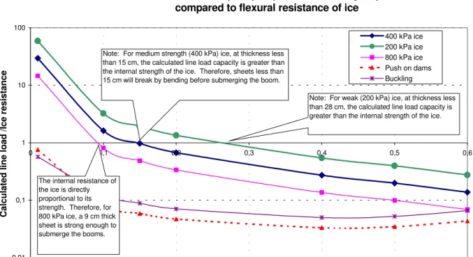
We note that as soon as the ice is at all thick, its flexural strength is greater than the boom's capacity to hold it back. Depending on the ice strength, the critical thickness is 9, 15 and 28 cm for ice 800, 400 and 200 kPa. So thin and weak ice sheets will fail in bending while thicker and stronger ice sheets submerge the booms rather than break. Also included in the figure is the boom's capacity to retain ice as compared with ice's internal resistance to failure by buckling. Two curves are provided. The first is based on the work done by Sodhi and Nevel (1980) as reported by Timco (1986, Figure 4):
5 . 0 2 3 ) ) 1 ( 12 ( .... 13 . 7 ν − = K EH CK F i i
where C is a dimensionless factor which depends on the structure's width and on the friction coefficient. For wide structures, we chose C between 1 to 2 depending on the value of µ . The figure demonstrates that for standard values of Young's modulus, for
Calculated line load capacity required to submerge a pontoon compared to flexural resistance of ice
0,01 0,1 1 10 100 0 0,1 0,2 0,3 0,4 0,5 0,6 Ice thickness (m)
Calculated line load /Ice resistance
400 kPa ice 200 kPa ice 800 kPa ice Push on dams Buckling Note: For medium strength (400 kPa) ice, at thickness less
than 15 cm, the calculated line load capacity is greater than the internal strength of the ice. Therefore, sheets less than 15 cm will break by bending before submerging the boom.
The internal resistance of the ice is directly proportional to its strength. Therefore, for 800 kPa ice, a 9 cm thick sheet is strong enough to submerge the booms.
Note: For weak (200 kPa) ice, at thickness less than 28 cm, the calculated line load capacity is greater than the internal strength of the ice.
ice thickness greater than 10 cm, the retaining force of the boom is 10 times less than the internal strength of the ice in buckling. Therefore when forces are large and the sheet is greater than 10 cm, the boom will submerge – the ice will not buckle.
Also shown in Figure 7.7 is the ratio of the boom's retention capacity as compared with extreme forces generated on dams in reservoirs as derived by Carter (1999):
25 . 1 250 .... 14 . 7 Fi = Hi
Clearly, equation 7.14 is derived for completely different conditions and from different principles. It is only included for sake of comparison of loads that are generated on wide flexible structures (booms) to those generated on wide fixed structures (dams). Depending on ice thickness, the load on booms is 0.05 to 0.1 times that on a fixed structure.
In interpreting Figure 7.7, one must also recall that the analysis was made for a 61 cm boom only. For larger booms, the retention capacity is approximately proportional to the buoyancy force at submergence. For a given pontoon density, the buoyancy force is proportional to the square of the pontoon's diameter.
8 Estimating ultimate applied loads: Methodology
8.1 From elements that occasionally break
8.1.1 Anchor cables
Applied forces are estimated using one of three methods. When a structural component breaks, we can assume that applied force is equal to the ultimate breaking strength of the component. Sometimes, this can be inferred with a fair degree of confidence. For example, the standard 2 inch diameter "6/19 bridge rope" (traditionally used for section cables and also previously used for anchor cables) has a specified breaking strength of 169 tons (1503 kN). Depending on production conditions, the actual breaking strength is probably 2% higher (1530 kN).
However, one must also factor in the condition of the element at the time of breakage. For example, in 1994-1995, a number of anchor cables broke at Lanoraie. They were about 8 years old. From experience, we know that these cables were weakened through fatigue some 2 m below the junction plate. So the strength of the cable at the time of the break is a guess. One could assume any value between 25% and 90% of the original value. In this case, Using an estimated value 75%, the applied load during 1994-95 was therefore in the order of 1530 x 75% = 1200 kN. This corresponds to a line load of 1200/122 m = 10,3 kN/m.
One can also infer applied loads when the cables don't break. Knowing the ultimate cable strengths, if the cables don't break, the applied loads were less than that value. For example, at Lavaltrie and Lanoraie, from their initial deployment in the late 1960's up to 1995, when the booms were made out of Douglas fir (14" x 22" x 30'), when the anchor cables were new, there were no breaks during many years of deployment. This leads to the conclusion that the applied line loads did not exceed 1530/122 = 12,3 kN/m.
8.1.2 Section cables
One must also take into account the way that the load is applied. The specified ultimate strengths are for cables loaded in tension only. Often, other loads are applied to the cables, particularly the section cables that hold the booms. The pontoons apply a load perpendicular to the axis of the cable and thereby add to the axial loads. The cable clamps wear the cable at the contact points reducing its strength by some value (2% to 10%?). Depending on the age of the cable, this reduction must be applied when a section cable breaks.
Other structural elements that have broken are the "fuses" installed on the section cables. The fuses are "weak links" installed between the junction plates and the section cables. They ensure that if the applied load is too large, the fuse blows before the anchor cable breaks. The inclusion of fuses was necessary at Lavaltrie and Lanoraie because the initial design of the boom was faulty. Under the original design, the same cable was used for anchor cables as was used for section cables. Without the fuses, given the fact that the load in the anchor cable is about 63% higher than in the section cables, it is obvious that the anchor cable will break before the section cables do.
This is highly undesirable because once an anchor cable breaks, its entire load is immediately transferred to the neighbouring anchor cable causing it to break too. The ensuing domino effect causes all anchor cables to fail in sequence causing a massive failure of the structure. This is what happened at Lavaltrie in 1994-1995. Since it is very difficult and expensive to replace the anchor cables with ones that have greater strength, we opted to insert fuses in the section cables so that they would break before the anchor cables would. The fuses have the appearance of a tension link. They were built and tested by a local contractor. Given that a fairly good quality control was used, the breaking load of the fuses is estimated at between 75 and 85 tons (670 to 760 kN). In both 1999 and 2000, fuses broke on the northern most section of the Lavaltrie boom. This corresponds to a line load of at least 6 kN/m.
(It should also be noted that we tried to increase the strength of the anchor cables by changing the cable from a "rope" to a "bridge strand" but we were limited by the size of the connection at the anchor itself. On the newly constructed Yamachiche boom, no fuses are required because the anchor cables are properly dimensioned to support at least 1.8 times the section cable strength).
8.1.3 Chains
There are also some 3 to 8 chains that break annually. Estimating the corresponding force is more difficult in this case for two reasons. First, two types of 7/8 inch chains are used. The most common is a grade 30 chain that has a working load limit (WLL) of 12,800 lbs (57 kN). However, there is also some grade 80 mixed in and it has a WLL of 34,200 lbs (152 kN). The specified breaking strength of chain is four (4) times the WLL. However, the actual breaking strength is not provided by the manufacturer. We will assume it is 2% higher. When a old chain breaks, we will assume it to be 3% lower. In this case, assuming a break in a grade 30 chain, the applied force in about 4x57x97% = 220 kN. This corresponds to a local line load of 220 kN per chain x 22 chains per section cable / (122 m per section cable) = 40 kN/m.
8.2 From mechanical means
The second way to estimate the ultimate applied load on the boom cables is through mechanical means. Since it is difficult to measure tensile forces, they are converted to compression forces through the use of a cage developed for that purpose. One end of
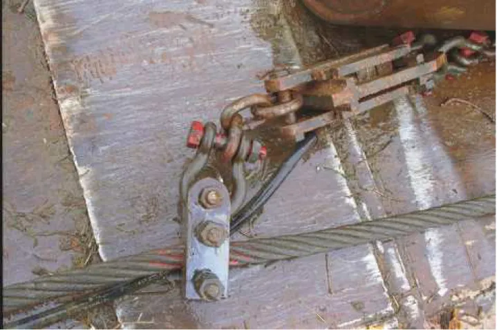
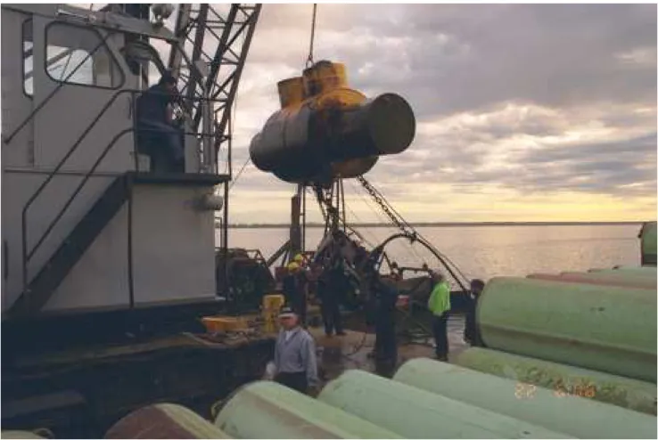
the cage fits into the junction plate while the other end is attached to the cable (see Figure 3.1). The cage is made in two parts such that it is possible to fit a ball bearing sandwich in the cage that will be compressed as the tension in the cable augments. Figure 8.2 and 8.3 show a small cage used to measure tensile forces on chains.
The sandwich is composed of two 2 cm thick pieces of aluminium about 7 cm by 7 cm square which hold three hard steel ball bearings in place forming an equilateral triangle. The bearings are about 1 cm in diameter and are prevented from moving around by the use of a foam keeping them in position. The more the sandwich is compressed the more the bearings are driven into the aluminium plates. Similar to the Brinell hardness test, the degree of penetration indicates the applied load. (Also in the cage is a load cell sampling the load twice a second that is connected to a data acquisition unit).
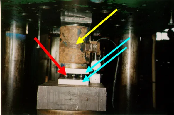
Figure 8.3 Load cell and ball bearing sandwich (for chains)
It shows the principle of converting tensile force acting on the chain into a compressive force within the cage. The two yellow (plain) arrows point to the two distinct parts of the cage. The blue arrows (with balls at the tail) point to the aluminium plates which form the sandwich. In between the plates are three ball bearings (not visible) which are compressed into the sandwich as the tensile forces in the chain increase. The red arrow (diamond at the tail) points to the load cell which is in series with the sandwich and is also compressed at the same time as the ball bearings. This particular instrument was set up on the prototype boom deployed during the winter of 1993-94. Very early in the season, the data communication cable between the load cell and the data acquisition CR10 unit broke and so no load cell data was retrieved. This particular instrument for forces on chains has not been deployed since.
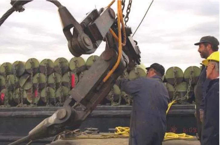
Figure 8.4 Typical load cell deployment at Yamachiche boom
(Note large cage for anchor cable (bottom) and smaller cages for section cables (top). Teflon-coated yellow armoured cables link load cells in cages to data acquisition unit in barrel (top out of view). Note pontoons in the background which will be deployed under the supervision of the foreman Georges Gouin (far right))
Figure 8.5 Load cells ready for deployment
(This is another view of the previous photo. Note the huge barrel which houses the CR10 data acquisition system and data transmission system. The domes on top of the barrel serve as antennas for real-time data transmission to a local booster station).