THESIS PRESENTED TO
ÉCOLE DE TECHNOLOGIE SUPERIEURE
IN PARTIAL FULFILLMENT OF THE REQUIREMENTS FOR THE DEGREE OF DOCTOR OF PHILOSOPHY
Ph.D.
BY
Amin KARBASSI
PERFORMANCE-BASED SEISMIC VULNERABILITY EVALUATION OF EXISTING BUILDINGS IN OLD SECTORS OF QUEBEC
MONTREAL, JULY 20, 2010
BY THE FOLLOWING BOARD OF EXAMINERS
Prof. Marie-José Nollet, Thesis Supervisor
Département de génie de la construction à l’École de technologie supérieure
Prof. Omar Chaallal, Internal Examiner
Département de génie de la construction à l’École de technologie supérieure
Prof. Patrick Terriault, President of the Board of Examiners
Département de génie mécanique à l’École de technologie supérieure
Prof. Luc Chouinard, External Examiner
McGill University – Department of Civil Engineering and Applied Mechanics
THIS THESIS WAS PRESENTED AND DEFENDED
BEFORE A BOARD OF EXAMINERS AND PUBLIC
June 15, 2010
To the survivors of the earthquake in Bam City, who have been always
the great examples of HOPE and INSPIRATION for me.
Here I get to this part of my thesis which comes at the beginning of the document, though it is really written as one of the last parts! This is probably because I wanted to make sure to remember everyone on the long list of names who not only gave me a hand in conducting this research work but also helped me to be where I am now. However, now I realize that if like movie credits, I want to mention everyone’s name, I will end up having several pages for this part. Emotions can also be involved as I am writing this page on the 5th anniversary of leaving home to come to Canada to pursue my PhD studies. Time passes fast, doesn’t it!
Getting to know Marie-José in the CSCE conference in 2002 was one of the greatest chances I have had in my academic life. Who knew that she would become my research supervisor three years later when I felt confident enough with my French language to come to École de technologie supérieure. Marie-José, I am really thankful for your academic advices, support, and kindness through all these 5 years which has made me think of you not only as my research supervisor but also as one of my best friends: how many supervisors in the world would come all the way down to their student’s apartment just after he arrives in town, on a Sunday afternoon, to make sure he has the necessary house stuff!
The days away so far from home would have not passed easy if I did not feel that I had the absolute emotional support of my family, whenever I needed it. Dad and Mom, although I will never be able to pay you back for what you have done for me, I want you to know that I am sincerely grateful for it. My brother Arsha and his wife Niloofar, though you still owe me a visit here, your remote support has been endless, and I am really thankful for that.
Finally, the word HOME has always been something unique for me. However, after living in the lovely city which they call it MONTREAL, I have come to this belief that home is any place where one can find peace and endless friendships, somewhere like Montreal! Whom can I thank for that?
Amin KARBASSI
ABSTRACT
To perform a seismic vulnerability evaluation for the existing buildings in old sectors of Quebec, two major tools at two different levels are missing: first, in the context of the seismic vulnerability assessment of a group of buildings, an updated rapid visual screening method which complies with the Uniform Hazard Spectra presented in the 2005 version of the National Building Code of Canada (NBCC) does not exist; and second, in the context of loss estimation studies, capacity and fragility curves which are developed based on the specific building typologies present in those sectors are required. In this research work, in the first place, a building classification for the existing buildings in old sectors of Quebec considering the masonry as the main construction material is proposed. Later, an updated rapid visual screening method—in the form of vulnerability indices for different typologies and cities in Quebec—which is adapted to the Uniform Hazard Spectra in NBCC 2005 is proposed. The structural vulnerability indices (SVI) are calculated through the application of the improved nonlinear static analysis procedure in FEMA 440 Improvement of nonlinear static seismic analysis procedures for three levels of seismic hazard. A set of index modifiers are also presented for the building height, irregularities, and the design and construction year. To deal with the second problem, on the other hand, a performance-based seismic vulnerability evaluation method is applied to examine the structural performance of two buildings—a 6-storey industrial masonry building and a 5-storey concrete frame with masonry infill walls, as two of the building classes constructed vastly in old sectors in Quebec—at multiple seismic demand levels. The results of such an assessment are used to develop dynamic capacity and fragility curves for the target buildings. The Applied Element Method is used here as an alternative to FE-based methods to conduct a thorough 4-step performance-based seismic vulnerability evaluation. To this end, the Incremental Dynamic Analyses (IDA) for the buildings are carried out using various sets of synthetic and real ground motions representing three M and R categories. Consequently, the fragility curves are developed for the three structural performance levels—Immediate Occupancy, Life Safety, and Collapse Prevention. Finally, the mean annual frequencies of exceeding those performance levels are calculated by combining the data from the calculated fragility curves and those from the region’s hazard curves. The proposed method is shown to be useful to conduct seismic vulnerability evaluations in regions for which little observed damage data exists.
Keywords: Applied Element Method, Masonry, Incremental Dynamic Analysis, Rapid Visual Screening, Performance-Based Seismic Evaluation
Amin KARBASSI
RESUMÉ
Actuellement, il manque deux outils importants et cela à deux niveaux différents pour l'évaluation de la vulnérabilité sismique des bâtiments existants dans les anciens quartiers du Québec. Premièrement, dans le cadre de l'évaluation de la vulnérabilité sismique d'un groupe de bâtiments, il n’y a pas de méthode d’attribution de pointage qui soit conforme aux spectres d'aléa uniforme de l’édition 2005 du Code national du bâtiment du Canada (CNBC). Deuxièmement, pour compléter des analyses d’estimation des dommages il est nécessaire de développer des courbes de capacité et de fragilité pour les typologies spécifiques de bâtiments qu’on retrouve dans les anciens quartiers. Dans ce travail de recherche, on propose d’abord une classification typologique des bâtiments existants des anciens quartiers du Québec considérant la maçonnerie comme matériau de construction principal. Par la suite, on propose une nouvelle procédure d’évaluation rapide sur la base d’indices de vulnérabilité sismique pour les différentes typologies et villes du Québec. Un niveau de sismicité (faible, modéré ou élevé) est attribué à chaque ville selon les valeurs d'accélération spectrale de l’édition 2005 du Code national du bâtiment du Canada. Pour chaque niveau de sismicité, des indices de la vulnérabilité sismique structurale (IVS) et des modificateurs (ceux-ci considèrent la hauteur du bâtiment, les irrégularités, et les années de conception et de construction) sont calculés à partir de la procédure d’analyse statique non-linéaire améliorée du FEMA 440 « Improvement of nonlinear static seismic analysis procedures ». Pour répondre à la deuxième problématique, une méthodologie basée sur les niveaux de performance est appliquée afin d’étudier la vulnérabilité sismique de deux bâtiments à de multiples niveaux de demande sismique. Deux classes de bâtiment présentes en grande proportion dans les anciens quartiers du Québec sont considérées, soient un bâtiment industriel en maçonnerie non armée de 6 étages et un cadre en béton armé avec des remplissages en maçonnerie non armée de 5 étages. Les résultats de cette évaluation sont utilisés pour développer les courbes de capacité dynamique et les courbes de fragilité de ces bâtiments. La méthode des éléments appliqués (MEA) est utilisée ici, comme une alternative aux éléments finis, afin de faire une étude d'évaluation en quatre (4) étapes. À cette fin, une série d’analyses dynamiques incrémentales temporelles (IDA) est réalisée en utilisant des accélérogrammes synthétiques et réels représentant trois combinaisons amplitude-distance (M et R). Les courbes de fragilité sont développées pour trois niveaux de performance structurale (occupation immédiate, sécurité des occupants, et prévention de l’effondrement). La fréquence annuelle moyenne de dépassement de ces niveaux de performance est ensuite calculée en combinant les données des courbes de fragilité à celles des courbes d’aléa de la région. Une comparaison des courbes de fragilité développées dans ce travail de recherche
avec les courbes de fragilité de HAZUS est présentée et les différences et les similarités sont discutées. Il est démontré que la méthode proposée ici est efficace pour réaliser des évaluations de vulnérabilité sismique dans les régions pour lesquelles il existe peu de données sur les dommages observés.
Mots-clés: méthode des éléments appliqués, maçonnerie, analyse dynamique incrémentale temporelle, méthode d’attribution de pointage, niveaux de performance
Page
INTRODUCTION………....……….1
CHAPTER 1 LITERATURE REVIEW ... 6
1.1 Introduction ... 6 1.2 Definition of terms ... 7 1.2.1 Seismic hazard ... 7 1.2.2 Seismic vulnerability ... 7 1.2.3 Seismic risk ... 7 1.3 Fragility curves ... 8
1.4 Seismic vulnerability methods ... 9
1.4.1 Observed damage data ... 13
1.4.2 Expert opinions ... 13
1.4.3 Simple analytical model ... 14
1.4.4 Detailed analysis ... 15
1.4.5 Score assignment procedures ... 22
1.5 Performance-based seismic vulnerability evaluation of existing buildings ... 28
1.6 Loss estimation analysis : mean annual frequency of exceeding damage states .... 29
1.7 State of the seismic vulnerability evaluation methods in Quebec ... 30
1.7.1 Building classification in Quebec ... 30
1.7.2 Applicability of existing seismic vulnerability methods for Quebec ... 33
1.7.3 Complexity level of analytical procedures for masonry buildings ... 34
1.8 Proposed methodology for the seimsic vulnerability evaluation of buildings with masonry in Quebec ... 38
1.9 Summary ... 39
CHAPTER 2 SCORE ASSIGNMENT METHOD ADAPTED FOR THE SEISMIC HAZARD IN QUEBEC ... 412
2.1 Introduction ... 422
2.2 Method development principles ... 422
2.3 Seismic hazard regions in Quebec ... 444
2.4 Basic assumptions in the calculation of indices ... 46
2.5 Development of index modifiers ... 53
2.6 Cutoff Index ... 58
2.7 Discussion of the SVI scores ... 60
2.8 Application of the proposed procedure ... 64
CHAPTER 3 PERFORMANCE-BASED SEISMIC VULNERABILITY EVALUATION OF BUILDINGS WITH MASONRY IN
QUEBEC: STRUCTURAL ANALYSE STAGE ... 67
3.1 Introduction ... 67
3.2 Description of the studied buildings ... 67
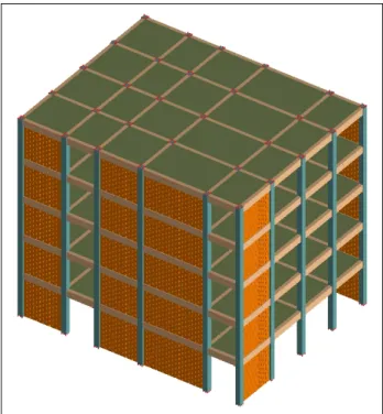
3.2.1 First studied building: unreinforced brick masonry (URMW) ... 68
3.2.2 Second studied building: RC frame with unreinforced masonry infill walls (CIW) ... 69
3.3 Analytical modeling ... 71
3.3.1 Application of the Applied Element Method for masonry ... 71
3.3.2 Application of AEM in the Incremental Dynamic Analysis ... 73
3.4 Structural analysis stage for the URMW building ... 74
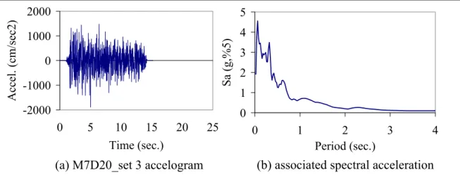
3.4.1 Time-history analysis of the building: selection of accelograms ... 74
3.4.2 Application of the Incremental Dynamic Analysis ... 79
3.4.3 Distribution of structural performance levels ... 80
3.5 Structural analysis stage for the CIW building ... 84
3.5.1 Time-history analysis of the building: selection of accelograms ... 84
3.5.2 Application of the Incremental Dynamic Analysis ... 87
3.5.3 Distribution of structural performance levels ... 88
3.6 Summary ... 90
CHAPTER 4 STRUCTURAL ANALYSIS RESULTS: DAMAGE ANALYSIS AND LOSS ANALYSIS STAGES ... 90
4.1 Introduction ... 90
4.2 Damage analysis for the URMW building... 90
4.2.1 Distribution of the structural performance levels ... 90
4.2.2 Development of the fragility curves for the URMW building ... 93
4.2.3 Combined fragility curves for the URMW building ... 98
4.3 Damage analysis for the CIW building ... 100
4.3.1 Distribution of the structural performance levels ... 100
4.3.2 Development of the fragility curves for the CIW building ... 102
4.4 Loss analysis stage: mean annual frequency of exceeding the damage states ... 104
4.4.1 URMW building ... 106
4.4.2 CIW building ... 109
4.5 Summary ... 1133
CHAPTER 5 DISCUSSION OF THE RESULTS ... 114
5.1 Introduction ... 114
5.2 Statistical analysis of the information obtained from the IDA curves ... 114
5.2.1 Unreinforced masonry building ... 114
5.2.2 RC frame building with unreinforced masonry infill walls ... 117
5.3.1 Unreinforced masonry building ... 119
5.3.2 RC frame building with unreinforced masonry infill walls ... 120
5.4 Comparing with HAZUS fragility curves ... 122
5.4.1 Unreinforced masonry building ... 122
5.4.2 RC frame building with unreinforced masonry infill walls ... 125
5.5 Application of the loss estimation studies in developing SVI ... 126
5.6 Application of the AEM in the progressive collapse of the studied structures ... 128
5.7 Standard error in the estimation of the measured values ... 129
5.8 Discussion on fragility curves : estimation of confidence intervals ... 131
5.9 Summary ... 133
CONCLUSION ... 135
RECOMMENDATIONS ... 140
APPENDIX I CLASSIFICATION OF CITIES IN QUEBEC ACCORDING TO THEIR SEISMIC HAZARD LEVEL ... 144
APPENDIX II VALIDATION OF THE APPLIED ELEMENT METHOD APPLICATION FOR NONLINEAR ANALYSIS OF CONCRETE AND MASONRY STRUCTURES ... 147
Page
Table 1.1 Selected references classified based on the assessment methodology ...12
Table 1.2 Building classification used in NRC-IRC (1992) ...24
Table 1.3 Building classification used in ATC (2002b) ...26
Table 1.4 Comparison of the current Canadian building classification with classes seen in old Montreal according to Lefebvre (2004) and Rodrigue (2006) ...32
Table 1.5 Proposed building classification for existing structures in historical areas of Quebec ...33
Table 2.1 Criteria for specifying the seismic hazard level for cities in Quebec taken from ASCE (1998) ...44
Table 2.2 Median of spectral acceleration values for different periods at different seismic hazard levels ...46
Table 2.3 Recommended damping values taken from Newmark and Hall (1982) ...49
Table 2.4 Suggested values for the elastic damping used in this chapter ...49
Table 2.5 Selection of the Canadian seismic design level as a function of the design date and the seismic hazard level ...51
Table 2.6 Structural vulnerability indices for different building classes in Quebec ...53
Table 2.7 Index modifiers for soil classes D and E ...54
Table 2.8 Index modifiers for plan irregularities ...55
Table 2.9 Index modifiers for vertical irregularities ...56
Table 2.10 Index modifiers for post-benchmark buildings ...57
Table 2.11 Index modifiers for pre-code buildings ...57
Table 2.13 Index modifiers for high-rise buildings ...58
Table 2.14 Example 1 building inventory used to evaluate the cutoff index ...59
Table 2.15 Example 2 building inventory used to evaluate the cutoff index ...59
Table 3.1 Structural characteristics of the building shown in Figure 3.1 ...69
Table 3.2 Material properties used in the Incremental Dynamic Analyses ...69
Table 3.3 Structural characteristics of the building shown in Figure 3.2 ...70
Table 3.4 Properties used for the concrete in the Incremental Dynamic Analyses ...71
Table 3.5 Characteristics of records used in the Incremental Dynamic Analyses ...75
Table 3.6 Spectral acceleration values of the target spectrum at different periods ...78
Table 3.7 Definition of Structural Performance levels taken from ASCE (2000) ...81
Table 3.8 Characteristics of synthetic ground motion records used in the Incremental Dynamic Analyses ...87
Table 3.9 Definition of buildings damage states taken from NIBS (1999) ...89
Table 4.1 The IM and DM values at the three performance levels of the URMW building in the longer direction ...91
Table 4.2 The IM and DM values at the three performance levels of the URMW building in the shorter direction ...92
Table 4.3 Logarithmic values of the URMW’s intensity measures in Table 4.1 for the three performance levels, in the longer direction ...95
Table 4.4 Logarithmic values of the URMW’s intensity measures in Table 4.2 for the three performance levels, in the shorter direction ...96
Table 4.5 Median and standard deviation values of ln[Sa(g)] shown in Tables 4.5 and 4.6 ...97
Table 4.6 Median and standard deviation values of ln[Sd(cm)] shown in Tables 4.5 and 4.6 ...97
Table 4.7 The IM and DM values at the three performance levels of the CIW building ...101
Table 4.8 Logarithmic values of the CIW’s intensity measures in Table 4.9 for
the three limit states ...103
Table 4.9 Median and standard deviation values for ln[Sa(g)] and ln[Sd(cm)], shown in Table 4.11 ...103
Table 4.10 Spectral acceleration values (g) with different probability of exceedance in La Malbaie, Quebec ...105
Table 4.11 MAF’s of exceedance and return periods of violating the performance levels, displacement in the longer direction (T=0.38 sec.) ...109
Table 4.12 MAF’s of exceedance and return periods of violating the performance levels, displacement in the shorter direction (T=0.69 sec.) ...109
Table 4.13 MAF’s of exceedance and return periods of violating the performance levels ...111
Table 5.1 Summary of the limit states in the URMW’s longer direction ...115
Table 5.2 Summary of the limit states in the URMW’s shorter direction ...116
Table 5.3 Summary of the limit states for the CIW building ...118
Table 5.4 Coefficient of variation for masonry buildings’ fragility curves in HAZUS (NIBS 2003) and those developed in Chapter 4 ...124
Table 5.5 Probability of exceedance of the Collapse Prevention level in 50 years, calculated from Tables 4.14 and 4.16 ...127
Table 5.6 Seismic Vulnerability Indices for the two studied buildings in this research work ...127
Table 5.7 Medians and standard errors of estimation of DM’s and IM’s of the URMW building at different performance states ...130
Table 5.7 Medians and standard errors of estimation of DM’s and IM’s of the CIW building at different performance states ...130
Table 5.8 90% confidence interval of the DM and IM median values for the CP damage state ...132
LIST OF FIGURES
Page
Figure 1.1 Example of fragility curves for unreinforced masonry buildings. ...9
Figure 1.2 Existing methods for the predicted vulnerability assessment. ...11
Figure 1.3 Basics of vulnerability assessment using analytical models. ...15
Figure 1.4 Coefficient method of displacement modification process. ...19
Figure 1.5 Graphical illustration of the Capacity-Spectrum Method. ...20
Figure 1.6 Failure modes in masonry walls observed in an earthquake. ...34
Figure 1.7 Modeling an element in AEM. ...36
Figure 1.8 Element shape, contact points, and degree of freedom in AEM. ...37
Figure 1.9 Spring distribution and area of influence of each springs pair in AEM. ...37
Figure 2.1 Essential elements for developing the tools for a score assignment method tools. ...43
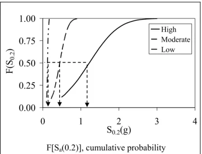
Figure 2.2 Distribution of spectral acceleration values at 0.2 sec, Sa(0.2), in different seismic hazard levels in Quebec. ...45
Figure 2.3 Distribution of spectral acceleration values at 1.0 sec, Sa(1.0), in different seismic hazard levels in Quebec. ...46
Figure 2.4 Graphical illustration of the Capacity-Spectrum Method. ...47
Figure 2.5 Example of fragility curves for unreinforced masonry buildings. ...50
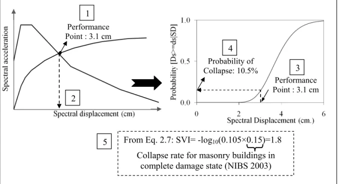
Figure 2.6 Graphical illustration of the process of calculating the BSH for the URM building class. ...52
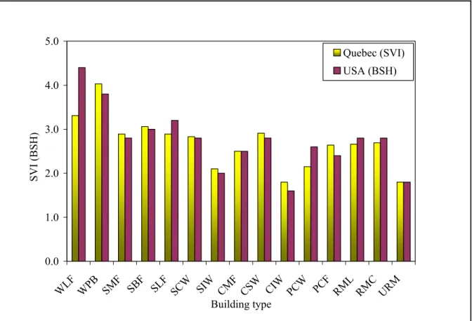
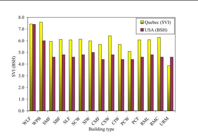
Figure 2.7 Comparison of the SVI in Quebec and the BSH scores in the USA, in regions with high seismic hazard. ...61
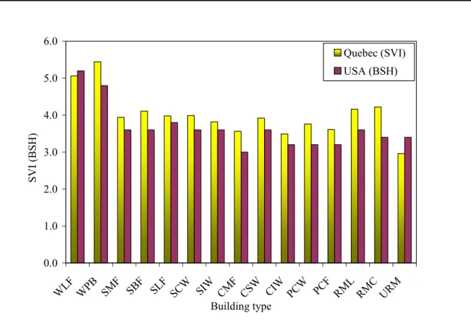
Figure 2.8 Comparison of the SVI in Quebec and the BSH scores in the USA, in regions with moderate seismic hazard. ...62
Figure 2.9 Comparison of the SVI in Quebec and the BSH scores in the USA,
in regions with low seismic hazard. ...63
Figure 2.10 Graphical illustration of the spectrum shape effect on the calculation of the performance point for WLF class. ...63
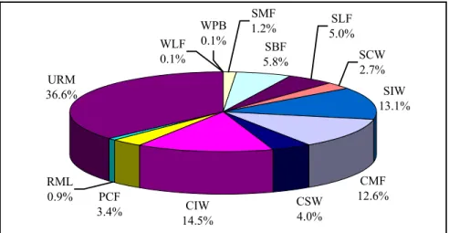
Figure 2.11 Distribution of building types in the Quebec City project. ...65
Figure 2.12 Distribution of collapse probability among existing building types in a damage scenario in the Quebec City project. ...66
Figure 3.1 Three-dimensional views of the unrienforced masonry structure. ...68
Figure 3.2 Three-dimensional views of the RC frame with unreinforced masonry infill walls. ...70
Figure 3.3 Modeling masonry in AEM. ...72
Figure 3.4 M6D30 set 1 time-history record used in the IDA of the URMW. ...76
Figure 3.5 M7D70 set 2 time-history record used in the IDA of the URMW. ...76
Figure 3.6 M7D20 set 3 time-history record used in the IDA of the URMW. ...77
Figure 3.7 Saguenay S7 time-history record used in the IDA of the URMW. ...77
Figure 3.8 5%-damped elastic response from records in Table 3.3 matched to the target spectrum. ...78
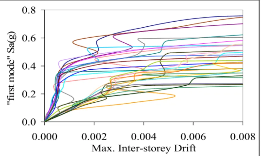
Figure 3.9 IDA curves for both the longer and shorter directions of the URMW building. ...80
Figure 3.10 IDA curve of the URMW building in the shorter direction for Nahanni ground motion. ...82
Figure 3.11 URMW building at Immediate Occupancy level for Nahanni S3-EN1 ground motion record. ...82
Figure 3.12 URMW building at Life Safety level for Nahanni S3-EN1 ground motion record. ...83
Figure 3.13 URMW building at Collapse Prevention level for Nahanni S3-EN1 ground motion record. ...83
Figure 3.14 Comparison of the spectral acceleration data for M6 at D20-30
ground motion records (Table 3.5) with the target spectrum in Table 3.6 ...85 Figure 3.15 Comparison of the spectral acceleration data for M7 at D15-25
ground motion records (Table 3.5) with the target spectrum in Table 3.6 ...85 Figure 3.16 Comparison of the spectral acceleration data for M7 at D50-100
ground motion records (Table 3.5) with the target spectrum in Table 3.6 ...86 Figure 3.17 Two-dimensional IDA curves for the CIW building. ...88 Figure 4.1 Distribution of the IO and CP performance levels on the URMW’s
IDA curves. ...93 Figure 4.2 Q-Q plots for the IM values at the Collapse Prevention level. ...94 Figure 4.3 Fragility curves for the three performance levels, URMW longer
direction. ...97 Figure 4.4 Fragility curves for the three performance levels, URMW shorter
direction. ...98 Figure 4.5 Upper (UB) and lower bounds (LB) of the fragility curves. ...100 Figure 4.6 Distribution of the IO and CP performance levels on the CIW’s
IDA curves. ...101 Figure 4.7 Q-Q plots for the IM values at the Collapse Prevention level. ...102 Figure 4.8 Acceleration-based fragility curves for the CIW building at the three
performance levels. ...104 Figure 4.9 Displacement-based fragility curves for the CIW building at the three
performance levels. ...104 Figure 4.10 Spectral acceleration curves with different probability of exceedance
in 50 years for La Malbaie, Quebec. ...106 Figure 4.11 Hazard curves at URMW building’s fundamental periods in the
longer and shorter directions. ...106 Figure 4.12 Lower bound of the combined fragility curves along with the hazard
Figure 4.13 The URMW building’s mean annual frequency of exceeding the
Immediate Occupancy performance level, due to Sa = z. ...107 Figure 4.14 The URMW building’s mean annual frequency of exceeding the
Life Safety performance level, due to Sa = z. ...108 Figure 4.15 The URMW building’s mean annual frequency of exceeding the
Collapse Prevention performance level, due to Sa = z. ...108 Figure 4.16 Hazard curves calculated at the CIW building’s fundamental periods
in the longer and shorter directions. ...110 Figure 4.17 The CIW building’s fragility curves along with the hazard curves at
the building’s dominant modes of vibration. ...110 Figure 4.18 The CIW building’s mean annual frequency of exceeding ...111 Figure 5.1 Summary of the URMW’s IDA curves into the median, 16%, and
84% fractiles. ...116 Figure 5.2 Summary of the CIW’s IDA curves into the median, 16%, and
84% fractiles. ...118 Figure 5.3 URMW’s maximum ISD of all storeys at different values of Sa(T1)
for set 1 ground motion record of category 3 in Table 3.5. ...119 Figure 5.4 IDA curves for each storey of the URMW building, for set 1
ground motion record of category 3. ...120 Figure 5.5 CIW’s maximum ISD of all storeys at different values of Sa(Tx)
for group 5 of the ground motion in Table 3.8. ...121 Figure 5.6 IDA curves for each storey of the CIW building, for group 5 of
the ground motion records. ...121 Figure 5.7 Fragility curves of the masonry building in the longer direction
compared with HAZUS fragility curves for a pre-code midrise URM. ...123 Figure 5.8 Fragility curves of the masonry building in the shorter direction
compared with HAZUS fragility curves for a pre-code midrise URM. ...123 Figure 5.9 Fragility curves of the concrete frame building compared with
Figure 5.10 The URMW 5% and 95% confidence-level fragility curves, for the
CP limit state. ...133 Figure 5.11 Upper and lower bounds of the 5% and 95% confidence-level URMW
LIST OF ACRONYMS AND INITIALISMS
AEM Applied Element Method BSH Basic Structural Hazard
ASCE American Society of Civil Engineering ATC Applied Technology Council
[C] Damping matrix
CIW RC frame with unreinforced masonry infill walls CP Collapse Prevention
DM Damage measure
E Young’s modulus
Eb Brick Young’s modulus ED Energy dissipated by damping Em Mortar Young’s modulus ESo Maximum strain energy FC Fragility curve FEM Finite Element Method
FEMA Federal Emergency Management Agency Δf(t) Incremental applied load vector
g Ground acceleration
G Shear modulus
Gm Mortar shear modulus
HC Hazard curve
IDA Incremental Dynamic Analysis IM Intensity measure
IO Immediate Occupancy ISD Inter-storey drift
[K] Stiffness matrix Kn Normal stiffness KNeq Equivalent normal stiffness Ks Shear stiffness
KSeq Equivalent shear stiffness
LS Life Safety
[M] Mass matrix
MAF Mean annual frequency MDOF Multi-degree-of-freedom MMI Modified Mercalli intensity NBCC National Building Code Canada
NIBS National Institute of Building Sciences NRCC National Research Council Canada PBSE Performance-based Seismic Evaluation PGA Peak ground acceleration
RG Residual force vector Sa Spectral acceleration Sd Spectral displacement SDOF Single-degree-of-freedom SI Structural index SPI Seismic priority index SVI Structural vulnerability index Te Effective period
Teq Equivalent period Ti Initial period
URMW Unreinforced masonry with wood floors USGS United States Geological Survey
[ΔU] Incremental displacement vector [ΔU'] Incremental velocity vector [ΔU"] Incremental acceleration vector
β Standard deviation
βeq Equivalent damping βeff Effective damping
Φ Lognormal-cumulative distribution
μ Median value
INTRODUCTION
In spite of all developments in the seismic design of new buildings in Canada in the recent years, it is important to know that the first detailed seismic provisions were not incorporated in the National Building Code of Canada until the 1950’s. This means that there are several structures, built before that time, which are not designed to resist earthquake loads. Consequently, human and economic losses can be high among those building stocks as a result of an earthquake in the future. Therefore, the same amount of attention that is given to the seismic design of new buildings should be paid to loss estimation of existing structures. Significant damages to structures built without seismic load resisting provisions have been observed in different parts of the world. The recent devastating earthquake in Haiti, in January 2010, is a clear example (USGS/EERI 2010).
Although the occurrence rate of earthquakes in Quebec is lower in comparison with the earthquake frequency in Western Canada, the social and economical impacts of earthquakes on buildings that have been built before the existence of seismic regulations in the province cannot be neglected. The seismic zone of Charlevoix (located at a 100km distance from Quebec City) is the most active zone in the east part of Canada. Five earthquakes with the magnitude of six or more (in 1663, 1791, 1860, 1870, and 1925) have occurred in the region1. Moreover, in the 20th century, three significant earthquakes—The 1925 Charlevoix-Kamouraska (Magnitude 6.2), The 1935 Timiskaming (or Témiscaming) (Magnitude 6.2), and The 1944 Cornwall-Massena (Magnitude 5.6)—have occurred in the province.
Defining the problem
Based on a study of the approximate distribution of seismic risk among Canada’s urban population due to the existing seismic hazard (probability of occurrence of an earthquake) (Adams et al. 2002) showed that Montreal and Quebec City are among the 6 most vulnerable
cities in the country. In this study, Vancouver is stated to have the highest population at risk, Montreal is placed second, and Quebec City is positioned in the 6th place.
In regions highly populated and constructed, such as Montreal and Quebec City, the seismic risk can be high especially among old masonry buildings because of the combination of seismic hazard with the vulnerability of such a building class and the social and cultural values of those ancient structures.
Masonry is considered the most important construction material in the world as it has been used in public and residential building construction over the past hundred years. Although some specific features have been added to improve the seismic behavior of masonry buildings during the course of time, such as the confined masonry construction and tying the walls, masonry constructions remain, even nowadays, the most vulnerable part of existing building stocks.
To evaluate the seismic vulnerability of a building stock and perform a loss estimation study, several approaches are available. Most of those approaches rely on having a clear building classification for the area and developing the corresponding fragility curves for each class. These curves give the probability of exceeding a particular damage state given a level of seismic demand. It has been shown in previous studies that the available building classifications in North America does not include all types of unreinforced masonry buildings present in old sectors of Quebec (Lefebvre 2004).
Taking into account the nonlinear dynamic behaviour of structures is essential for developing precise fragility curves for existing buildings. However, the dynamic structural analysis of unreinforced masonry buildings faces several challenges: because of the brittle properties of brick units and mortar joints, the overall behaviour of masonry units is often considered linear; nevertheless, the masonry units are shown to have an explicit nonlinear behaviour in progressive collapse cases (Colliat et al. 2002). Consequently, fragility curves should reflect
this nonlinear behaviour. Nonetheless, the difficulties to represent the global dynamic behaviour of masonry structures in an accurate way, stated in the literature, questions the validity of the available fragility curves for masonry buildings, developed by static pushover analysis.
Objectives, applied methodology, and originality
The main objective of this research work is to develop a predicted-based seismic vulnerability evaluation method for buildings with masonry construction in old sectors of Quebec. The focus will be on two types of masonry buildings: (1) unreinforced brick masonry buildings with wood floors (URMW) which represent the structures in the old industrial sectors in Montreal and Quebec City at the beginning of the century, and (2) RC frames with unreinforced masonry infill walls (CIW) which used to be a very popular building type between 1930 and 1950 in Quebec. The main objective is achieved at two levels. First of all, a rapid visual screening method compatible with the regional seismic hazard of the province is developed, and second, the dynamic capacity and fragility curves for buildings with unreinforced brick masonry are established considering the nonlinear dynamic behaviour of the masonry.
To achieve the objective of this study, the following methodology is followed.
1. Reviewing the existing seismic vulnerability evaluation methods used in different part of the world.
2. Proposing a building classification that properly categorizes the existing ancient structures in Quebec, based on their structural characteristics and constructional materials.
3. Establishing a vulnerability scoring system or index calculation, compatible with the seismic demand in Quebec.
4. Calculating the “dynamic” capacity and fragility curves for the most frequently seen classes in old sectors in Quebec (masonry and concrete building with masonry infill walls).
The last step represents the main effort in this research thesis. The methodology used to calculate the dynamic capacity and fragility curves for the studied buildings consists of the most original contribution of this research work which is:
1. Applying the Applied Element Method to overcome the problems one would encounter when using a FE-based method in the dynamic analyses of masonry buildings. This method is based on dividing structural members into virtual elements connected through springs, and is used in this research work as an alternative to Finite Element Method (FEM) to model the progressive collapse in brick masonry in an adequate way.
2. Replacing the conventional dynamic analysis methodology by an Incremental Dynamic Analyses approach, when calculating the capacity and fragility curves because the later is shown to be an effective tool for thoroughly examining the structural performance of buildings under seismic loads (Christovasilis et al. 2009; Lagaros 2009).
3. Using the latest regional seismic demands for Quebec, presented in the 2005 edition of the National building code of Canada (NBCC) (NRCC 2005) in the form of spectral acceleration response values.
Organization of the thesis
Various seismic vulnerability evaluation methods which are currently in use in different parts of the world are reviewed in Chapter 1, and the essential elements for a suitable seismic vulnerability evaluation method in Quebec are identified and discussed. Based on such a literature review, a new building classification is proposed for the existing buildings in the old sectors of the province. Later on in Chapter 2, the procedure to develop a score assignment method which is adapted to the seismic demand in the province, for the seismic vulnerability evaluation of a group of buildings in old sectors of Quebec is explained.
Chapter 3 explains a performance-based seismic vulnerability evaluation to develop the dynamic capacity and fragility curves for two target buildings in this study. This section of the research work aims to overcome the lack of appropriate capacity and fragility curves, unavailable in the literature, for buildings with masonry construction in Quebec. The results obtained from such a methodology is presented in Chapter 4 for a typical unreinforced brick masonry building and a RC frame with unreinforced masonry infill walls, in Quebec, and a set of fragility curves are calculated for each building. In the context of loss estimation, the return period of exceeding the performance levels considered in this study is also calculated in the same Chapter. In Chapter 5, the results of the Incremental Dynamic Analyses are used to study the local dynamic behaviour of the buildings. Moreover, the fragility curves calculated in Chapter 4 are discussed in further details. Finally, the summary of the study along with recommendations for future works are presented in Chapter 6.
CHAPTER 1
LITERATURE REVIEW
1.1 Introduction
Different types of seismic vulnerability evaluation studies may be used depending on the nature of the problem at hand and the purpose of the study (Coburn and Spence 2002). These are:
1. Scenario studies, in which the effect of a single earthquake is calculated on a region (Fah et al. 2001). Major historic earthquakes are modeled to assess their effects on present-day portfolios to evaluate the resources that would be needed to withstand disasters such as those that occurred in the past, should similar ones occur in the future.
2. Probabilistic risk analysis, in which potential losses from different sources are calculated along with their probability of occurrence for an individual building, group of buildings, or for a region (Shaw et al. 2007). The latest can be performed when a clear building classification exists for the building stock. The results of such studies can be used to develop loss exceedance probability curves, which illustrate the level of loss that would be experienced with different return periods.
3. Potential loss studies, in which the effect of expected hazard levels across a region or country is mapped in order to show the locations of probable heavy losses to identify high-risk areas (Tantala et al. 2000).
One of the key elements in every study of this type is the assessment of the seismic vulnerability of the population of buildings under investigation. In this regard, a clear definition of the terms frequently used in those studies would be helpful for the reader.
1.2 Definition of Terms
1.2.1 Seismic Hazard
In seismic engineering, the term Hazard is defined as «the probability of occurrence of an earthquake with a certain severity, within a specific period of time, at a given location » (Coburn and Spence 2002). The earthquakes can be specified in term either of their source characteristics (e.g., magnitude) or their effect on a specific location (e.g., intensity or peak ground acceleration). In either case, the annual recurrence rates are usually used. The inverse of this term is called the average return period.
1.2.2 Seismic Vulnerability
Seismic Vulnerability is defined as the degree of exposure to loss (as the ratio of the expected loss to the maximum possible loss) for a given item at risk, ensuing from the occurrence of a specific level of seismic hazard. According to the characteristics of the element at risk, the measure of loss can be the casualty number, number of injuries or repair cost ratio. In a large population of buildings, this term may be defined as the proportion of buildings experiencing some particular level of damages.
1.2.3 Seismic Risk
This term refers to the potential economic, social and environmental consequences of an earthquake in terms of probable physical damages to properties, human losses, and injuries that may occur over a specific future time-period. The loss and physical damage elements are key points in the definition. In a region with a high seismic hazard in which there are no people or property that could be injured or damaged by an earthquake, the seismic risk is zero.
Based on the definition stated for each term, the seismic risk for a building (or a group of buildings) can be calculated as follows.
Seismic risk = Seismic hazard× vulnerability× value (1.1)
The seismic risk in a region is defined as the probability of occurrence of an earthquake with a certain magnitude, times the probability of damage caused by that earthquake (seismic vulnerability) times the economical or social value of the building(s) at risk.
1.3 Fragility Curves
The fragility curve for a building presents the probability of exceeding a damage state D (e.g., Collapse Prevention level), given intensity measure IM (e.g., spectral acceleration or spectral displacement) Therefore, the fragility curve is presented in the form of a two-parameter lognormal distribution function as follows.
− Φ = > = σ μ ) ln( ) ( ) (X P d D X F (1.2)
In Equation 1.2, Φ is the standard normal cumulative distribution function, X is the distributed intensity measure (e.g., Sa or Sd), and μ and σ are the median and standard deviation of the natural logarithm of the intensity measures, respectively. Figure 1.1 shows an example of the fragility curves for a masonry building in terms of its spectral displacement.
0 20 40 60 80 100 0 5 10 15 20 Spectral displacement (cm.) Pro bab ili ty [D s>=ds |S D ] Slight Moderate Extensive Complete
Figure 1.1 Example of fragility curves for unreinforced masonry buildings.
1.4 Seismic Vulnerability Assessment Methods
It is seen from Equation 1.1 that one of the key elements in every loss estimation study is the assessment of the seismic vulnerability of the building population under investigation. There are two principal methods used in the seismic vulnerability assessment of existing buildings, one of which is known as the observed vulnerability procedure and the other, as the predicted vulnerability method (Sandi 1982). The later is based on a combined use of analytical modelling and expert opinions.
The observed vulnerability assessment is based on the statistics of past earthquake damages. These can be accompanied by the opinion of experts and used to derive damage probability matrices (DPMs) which describe the probability that a building class is in a specific damage state for a given level of hazard. Such a procedure is suitable for non-engineered structures
whose earthquake resistance is difficult to calculate but for which, substantial statistical damage data exist.
In the absence of sufficient observed data, the predicted vulnerability assessment is applied to evaluate the seismic vulnerability of buildings. This method evaluates the expected performance of building classes based on calculations and design specifications. The assessment can be performed using either simple analytical models (D'Ayala et al. 1997) or detailed analysis procedures (Decanini et al. 2004), depending on the objective of the particular evaluation. Simple analytical models are applicable where the procedure’s precision is not as important as its rapidity. Detailed analysis methods, generally used for the evaluation of individual building, are not suitable for earthquake scenario projects where a large number of buildings have to be evaluated. However, they can be used to generate fragility curves for typical buildings from which one can either perform a loss estimation analysis or develop scores that correlate potential structural deficiencies with structural characteristics for different building classes. This is the basis for a seismic vulnerability assessment method called the score assignment, which will be explained in further detail in the next chapter. In situations where there is a lack of sufficient observed earthquake damage data, such as in the province of Quebec, the predicted vulnerability technique, coupled with a score assignment procedure, can be a suitable method for the seismic vulnerability evaluation of a group of buildings. Figure 1.2 shows the different available methods to conduct a predicted-based seismic vulnerability assessment for existing buildings as a group or individually.
Figure 1.2 Existing methods for the predicted vulnerability assessment.
Table 1.1 summarizes a number of references studied in this chapter as part of the literature review, based on their assessment methodology. Each method is described in the following sections.
Predicted Vulnerability Expert Opinion
(building group)
Simple analytical modeling (building group/individual)
Score assignment (vulnerability index) (building group)
Detailed modeling (individual building)
Table 1.1 Selected references classified based on the assessment methodology Observed Vulnerability Expert Opinions Simple Analysis Models Score Assignment Detailed Analysis (NRC-IRC 1992) --- --- --- √ ---
(McCormack and Rad
1997) --- √ --- √ --- (D'Ayala et al. 1997) --- --- √ --- --- (Faccioli et al. 1999) --- --- √ √ --- (Tantala et al. 2000) --- √ --- --- --- (Onur 2001) --- √ --- --- --- (D'Ayala and Speranza 2001) √ --- √ --- --- (ATC 2002a) --- --- --- √ --- (D’Ayala and Speranza 2002) --- --- √ --- --- (Lang 2002) --- --- √ --- --- (ASCE 2003) --- --- --- --- √ (Rossetto and Elnashai 2003) √ --- --- --- --- (Cohen et al. 2004) --- --- --- --- √ (White et al. 2005) --- --- --- √ --- (Valluzzi et al. 2005) --- --- √ --- ---
(LeBoeuf and Nollet
2006) --- --- --- √ --- (Belmouden and Lestuzzi 2007) --- --- --- --- √ (Calderini and Lagomarsino 2008) --- --- --- --- √ (Christovasilis, Filiatrault et al. 2009) --- --- --- --- √
1.4.1 Observed damage data
To define a relationship between earthquake damages and earthquake intensity, a substantial quantity of data is requires. Such equations are only valid for the original region or for areas with similar building population. However, if the calculated equation acknowledges the seismic resisting system of damaged buildings, seismic design practices in the region, and the building’s characteristics such as height and the number of storeys, then the equation can be used in the seismic assessment of other buildings with similar structural characteristics but in a different region (Rossetto and Elnashai 2003). The reason lies in the fact that there are such structural uncertainties in deriving those equations that any differences in construction practices and detailing between different regions are overcome.
1.4.2 Expert opinions
The observed vulnerability assessment method is the basis for the ATC 13 report, Earthquake damage evaluation data for California (ATC 1985), which provides experts’ damage estimations that can be used to evaluate the local, regional, and national economic impacts of earthquakes in California. The report essentially derives damage probability matrices for 78 different facility classes, 40 of which refer to buildings by asking 58 experts to estimate the expected level of damage that a specific structural class would undergo if subjected to a Modified Mercalli Intensity (MMI) from VI to XII. However, in addition to the uncertainties due to the variability in the buildings actual performance inherent in any estimation of damages, there are uncertainties related to opinions of the experts.
These damage probability matrices can not be easily calibrated or modified to incorporate new data and technological innovation (Porter et al. 2000) and it is difficult to extend the results to other building classes in other regions that have different construction practices, which include different construction details, building code requirements, construction materials, and workmanship quality.
Similar to ATC 13 methodology, damage probability matrices (DPM) have been developed for 31 building classes in British Columbia (Ventura et al. 2005). This study started with a
preliminary investigation of the seismic vulnerability of the general building stock in British Columbia using ATC-13 methodology as a benchmark, i.e., surveying local engineers. To this end, the building classes in ATC-13 were included in the survey and experts were asked to provide their opinions about the existence of each building class in British Columbia. The numbers of occurrences were categorized as low (0 to 10 occurrences), medium (10 to 50 occurrences), or high (more than 50 occurrences). Out of the 40 original building classes, 11 were chosen as the most prevalent in British Columbia. Following up on this initial work, a more comprehensive classification system including 31 building classes was developed to encompass the local building inventory.
1.4.3 Simple Analytical model
In the absence of observed damage data to generate vulnerability functions, other methods are required to assess the vulnerability of existing buildings. In assessing the vulnerability of a group of buildings, those methods should be able to analyse a large number of buildings in a short amount of time. To this end, analytical methods including simple models of buildings which require a few input parameters can be applied. To make the results reliable, those input parameters must be able to model the general seismic behaviour of the buildings.
Application in Europe
Examples of such a methodology are the seismic vulnerability assessments based on the identification of potential collapse mechanisms, expressed as the critical acceleration (D'Ayala et al. 1997; Faccioli et al. 1999). This method was applied in the seismic vulnerability assessment for a group of buildings in a historical center in the Umbria region in Italy (Valluzzi et al. 2005). A collapse coefficient equal to a/g (the mass multiplier able to led the building’s elements (walls, floors, and roofs) to failure) was presented for each building class. Such a multiplier was calculated based on reaching the upper limit of the equilibrium conditions (for out-of-plane and in-plane mechanism) rather than the maximum strength of the materials.
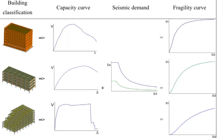
Analytical models can be applied to define the capacity curves of buildings that typify given building classes. These curves are then combined with the seismic demand (Figure 1.3) to produce the fragility curves for each of the building classes according to damage states definitions. Within the scope of the seismic vulnerability evaluation of existing buildings, Lang (2002) presents a simple and effective evaluation method for masonry and concrete buildings derived from analytical models. The method considers the nonlinear deformation capacity of the buildings under study; however, it misses to consider the dynamic properties of the materials under seismic loads. Moreover, the method can be time-consuming for buildings with numerous openings.
Figure 1.3 Basics of vulnerability assessment using analytical models.
1.4.4 Detailed analysis
A detailed analysis evaluation is necessary for potentially hazardous buildings which have been flagged in the rapid screening step of a multi-phase seismic assessment procedure. This method is not suitable for earthquake scenario projects where a large number of buildings have to be evaluated. However, the procedure can be used to improve the results of simple analytical methods. Detailed analyses are also helpful for developing fragility curves of buildings which typify a building class. The methodology can be divided into linear (static or dynamic) or non-linear categories (static or dynamic).
Target
building Capacity curve Seismic demand Fragility curve
Linear static analysis
A linear procedure maintains the traditional use of a linear stress-strain relationship; however, to consider the nonlinear characteristics of a building’s seismic response in such a procedure, adjustments to the building’s deformations and material acceptance criteria are incorporated (ASCE 2000). In a linear static procedure, the building is modelled as an equivalent single-degree-of-freedom (SDOF) system with a linear elastic stiffness and an equivalent viscous damping. The seismic input is modelled by an equivalent lateral force with the objective to produce the same stresses and strains as the earthquake it represents. The equivalent lateral force is determined from the response spectrum (acceleration) of the fundamental vibration mode, multiplied by the building’s mass. This corresponds to the typical formula to calculate the lateral force, in the seismic design codes.
V = m.Sa. C (1.3)
As shown in Equation 1.3, the second order effects such as stiffness degradation and force reduction due to anticipated inelastic behaviour are taken into account by the seismic coefficient C. This lateral force is then distributed over the height of the building and the corresponding internal forces and displacements are determined using linear elastic analysis. The results of linear procedures can be very inaccurate when applied to buildings with highly irregular structural systems, unless the building is capable of responding to the design earthquake(s) in a nearly elastic manner.
Linear dynamic analysis
Static procedures can be useful only when higher mode effects are not significant. This is generally true for short, regular buildings; otherwise, a dynamic procedure is required for buildings with irregularities (ASCE 2000). In the linear dynamic procedure, the building is modelled as a multi-degree-of-freedom (MDOF) system with a linear elastic stiffness matrix and an equivalent viscous damping matrix. The seismic input is modelled using either modal spectral analysis or time history analysis. In either case, the corresponding internal forces and
displacements are determined using linear elastic analysis. The advantage of a linear dynamic procedure with respect to a linear static one is that higher modes can be taken into consideration in the former. However, they are based on linear elastic response and hence, the applicability decreases in predicting the damage levels in the buildings in progressive collapse cases such as for masonry or concrete structures in an earthquake. Linear procedures are only applicable when the structure is expected to remain nearly elastic for the level of ground motions or when the design results in nearly uniform distribution of nonlinear response throughout the structure. However, from a performance point of view, greater inelastic demands are expected to be applied to the structure. Therefore, the uncertainty with linear procedures increases up to a point at which a high level of conservatism in demand assumptions and acceptability criteria is required to avoid unintended performance (ATC 2005). The procedures incorporating inelastic analysis can reduce such uncertainty and conservatism.
Nonlinear static analysis
In a nonlinear static procedure, the building is modeled as a SDOF structural system. The seismic ground motion, on the other hand, is represented by a demand parameter such as the spectral acceleration response. Subsequently, story drifts and component actions are related to the demand parameter through the pushover or capacity curves. Those capacity curves are generated by subjecting the structural model to one or more lateral load patterns (vectors) and then increasing the magnitude of the total load to generate a nonlinear inelastic force-deformation relationship for the structure at a global level. The load vector is usually an approximate representation of the relative accelerations associated with the first mode of vibration of the structure.
Two main applications of such a procedure are known as (i) the Coefficient Method of Displacement Modification presented in FEMA 356, Pre-standard and Commentary for the Seismic Rehabilitation of Buildings (ASCE 2000) and (ii) the Capacity-Spectrum Method of Equivalent Linearization presented in ATC 40, Seismic Evaluation and Retrofit of Concrete
Buildings (ATC 1996). In the Coefficient Method of Displacement Modification, the total maximum displacement of the SDOF system is estimated by multiplying the elastic response, based on the initial linear properties and damping, by a series of coefficients (C0 through C3). At the first step, an idealized force-deformation curve (pushover) relating the base shear to roof displacement should be produced (Figure 1.4). An effective period, Teff, is generated
from the initial period, Ti, by a graphical procedure to take into account some losses of
stiffness in the transition from elastic to inelastic behaviour. The peak elastic spectral displacement is directly related to the spectral acceleration (obtained from the response spectrum) through Equation 1.4.
) ( 4 2 . 2 . eff a eff d S T T S π = (1.4)
The final displacement is calculated through Equation 1.5.
δt = C0.C1.C2.C3.Sd (1.5)
In this equation, C0 is the shape factor, C1 is the dynamic load factor, C2 implements the
effect of pinching in load-deformation relationship due to degradation in stiffness and strength, and C3 applies the P-Δ effect. The values of each coefficient can be calculated from
Figure 1.4 Coefficient method of displacement modification process. Taken from ATC (2005)
The other method of the nonlinear static analysis, the Capacity-Spectrum Method of Equivalent Linearization, was first introduced by Freeman et al. (1975) as a rapid evaluation procedure in a pilot project for assessing the seismic vulnerability of buildings. The method assumes that the maximum total deformation (elastic and inelastic) of an SDOF system can be estimated from the elastic response of a system that has a larger period and greater damping than the original structure. The process begins with developing a force-deformation relationship (pushover curve) for the structure. To compare such a pushover curve with the seismic demand, as shown in Figure 1.5, the next step is to convert the force-formation capacity curve to an acceleration-displacement response spectrum.
In this format, period is represented as radial lines emanating from the origin. The equivalent period, Teq, is assumed to be the secant period at which the seismic ground motion demand, reduced for the equivalent damping, intersects with the capacity curve (Capacity Spectrum) at the performance point. It is also assumed that the equivalent damping of the system is associated with the full hysteresis loop area, as shown by the shaded area in Figure 1.5. As the equivalent period (Teq) and damping areas (ED) are both functions of the displacement, the solution to determine the maximum inelastic displacement is therefore iterative. This is
the basis of the simplified analysis methodology presented in ATC 40 to determine the displacement demand imposed on a building expected to deform inelastically.
Figure 1.5 Graphical illustration of the Capacity-Spectrum Method. Taken from ATC (2005)
Recent studies (Chopra and Goel 2000; ATC 2005; Powell 2006) indicate that the capacity spectrum method implemented in ATC 40 leads to very large overestimations of the maximum displacement for relatively short-period systems (i.e., periods shorter than about 0.5 s which relates to low and medium height buildings). Estimated maximum displacements in this period range can be, on average, more than twice as large as real maximum displacements. It is also shown that the procedure generally underestimates, by 30%, the maximum displacements of systems with periods greater than 0.5s. The results of an effort to improve the capacity spectrum method of ATC 40 are presented in FEMA 440, Improvement of Nonlinear Static Seismic Analysis Procedures (ATC 2005). The resulting suggestions focus on improved estimations of the equivalent period and damping. Similar to the current
ATC 40 procedure, the modified procedure’s effective period and damping both depend on the ductility, and so an iterative or graphical technique is required to calculate the performance point. The improved procedure is similar in application, to the current ATC 40 capacity spectrum method, and is used in this research work (explained in more details in Chapter 2) to develop the scores for a modified index assignment procedure in Quebec.
The current nonlinear static procedures based on invariant loading vectors such as those recommended in FEMA 356 or ATC 40 are shown to possess inherent drawbacks in adequately representing the effects of varying dynamic characteristics during the inelastic response of structures (Kunnath and Kalkan 2005). Although some improved nonlinear static procedures have been developed over the past few years (such as those in FEMA 440), their validity for a variety of structural systems and a range of ground motion characteristic have yet to be demonstrated. The results of nonlinear time history analyses based on actual earthquake recordings serve as the only reliable benchmark solutions against which the NSP results can be compared.
Nonlinear dynamic analysis
In a nonlinear dynamic analysis, a detailed structural model is subjected to a ground-motion record to produce estimates of the components deformations for different degrees of freedom. The modal responses at those degrees of freedom are then combined using schemes such as the square-root-sum-of-squares. This method is the most sophisticated analysis procedure for developing fragility curves of buildings which typify a building class. Because the calculated responses are sensitive to the characteristics of the individual ground motion used as the seismic input, different ground motion records are required to obtain a good estimation of the building’s responses. To this end, the Incremental Dynamic Analysis (IDA) has emerged as a potential tool for seismic evaluation because it applies a series of time history analyses.
Incremental Dynamic Analysis
An IDA involves subjecting a structural model to various ground motion records, each scaled to multiple levels of intensity up to the point at which a collapse limit state is reached (Vamvatsikos and Cornell 2002). Therefore, the IDA method is often described as a “dynamic” pushover procedure. The approach has the potential to demonstrate the variation of structural responses, as measured by a damage measure (DM, e.g., inter-storey drift), versus the ground motion intensity level, measured by an intensity measure (IM, e.g., peak ground acceleration or the first-mode spectral acceleration). The IDA procedure provides dynamic capacity curves for different ground motion levels. Although it is possible to utilize a single record for IDA, it is essential to consider variations in ground motion content when utilizing IDA in performance-based assessment. For this reason, the selection of ground motion records that takes into consideration site characteristics and source mechanisms is critical. This will be discussed in Chapter 2 where the IDA method is applied to develop the fragility curves for two building classes in Quebec.
1.4.5 Score assignment procedures
The score assignment procedure aims to identify seismically hazardous buildings by exposing structural deficiencies. Potential structural deficiencies and structural characteristics are correlated for different building classes using certain sets of scores that are usually calibrated by experts or analytical models. In most cases, these scores do not have a probabilistic meaning, and can just be used to prioritize buildings with respect to the probability of collapse.
Score assignment procedure in Canada
The rapid visual screening (RVS) method in Canada is described in the Manual for Screening of Buildings for Seismic Investigation (NRC-IRC 1992). As shown in Table 1.2, 15 building classes are introduced in this manual based on the construction material and the seismic
resistance system. The seismic screening procedure examines a building’s seismicity, soil condition, structure type, structural irregularities, presence of non-structural hazards, usage, and occupancy to determine its seismic priority index (SPI). The SPI is the sum of a building’s structural index (SI) and non-structural index (NSI), and it is a measure of the building’s deviation from the National Building Code of Canada 1990 (NRCC 1990) seismic requirements. Buildings are then ranked according to their respective scores and divided into low-, medium-, or high-risk categories. An SPI higher than 20 is an indication that the building requires a detailed investigation. The 15 building types described in this procedure have been defined based on previous work done by the Applied Technology Council of California (ATC 1998), and are presented in Table 1.2.
The current rapid visual screening method in Canada is based on seismic requirements of NBCC 1990; therefore, the indices in this manual would not fully comply with NBCC 2005 (NRCC 2005) requirements. Some research works have been conducted (Karbassi and Nollet 2008; Turenne 2009) to adapt this screening method to the 2005 version of NBCC. The structural indices in the current Canadian manual do not provide any probabilistic interpretation, and were developed mainly by considering the different base-shear force calculation concepts described in different versions of the NBCC. Later in Chapter 2, we will develop an index assignment procedure which is compatible with the regional seismic hazard in Quebec. The procedure is published in a paper by Karbassi and Nollet (2008).
Table 1.2 Building classification used in NRC-IRC (1992) Class Structural Description
WLF Light wood frame WPB Wood post and beam
SMF Steel Moment resisting frame SBF Steel braced frame
SLF Steel light frame
SCW Steel frame with concrete shear wall SIW Steel frame with infill masonry wall CMF Concrete moment resisting frame CSW Concrete shear wall
CIW Concrete frame with unreinforced masonry infill PCW Prefabricated concrete wall
PCF Prefabricated concrete frame
RML Reinforced masonry bearing walls with wood or metal diaphragms RMC Reinforced masonry bearing walls with concrete diaphragms URM Unreinforced masonry bearing walls
Score assignment procedure in the United States
The RVS of buildings for potential seismic hazards was initiated in 1988 with the publication of FEMA 154, Rapid Visual Screening of Buildings for Potential Seismic Hazards: a Handbook, (ATC 2002a) and its companion, FEMA 155, Supporting Documentation (ATC 2002b), both of which were updated in 2002. A major improvement in this update was to link the FEMA 154 screening results to FEMA 310, Handbook for the Seismic Evaluation of Buildings - A Pre-standard (ASCE 1998) and FEMA 356. To this end, the seismic hazard level was changed from 10% probability of being exceeded to 2%, in 50 years. Table 1.3 shows the acronym and description of the building classes considered in the latest version of this manual.
FEMA 154 procedure starts with a visual observation to identify the primary structural lateral-load resisting system based on the construction materials used (Table 1.3). Based on the identified structural system, the next step is to assign a Basic Structural Hazard score (BSH) to each building. The BSH is related to the probability of collapse in a building as a result of earthquakes in the future. As shown in Equation 1.6, the probability of collapse for a building is the product of the probability of the building being in the complete damage state multiplied by the fraction of buildings (of that class) which collapse when in the complete damage state.
BSH =-Log10[P(Complete Damage State)×P(Collapse | Complete Damage State)] (1.6)
In the first edition of FEMA 154, the BSH scores were calculated from the damage probability matrices of ATC 13. In the later edition, however, these probabilities are calculated from the fragility curves presented in the Earthquake Loss Estimation Methodology Technical Manual (NIBS 1999).
Finally, the overall score S (Equation 1.7) is calculated by modifying the BSH scores using a set of score modifiers which take into account some structural and site characteristics that are not considered in the calculation of the BSH scores and can be listed as follows.
1. Building’s height (midrise and highrise): BSH scores are calculated for lowrise buildings. 2. Vertical and horizontal irregularities.
3. Design and construction year for pre-code and post-benchmark buildings.
4. Buildings constructed on sites with soil classes C, D, or E: BSH scores are calculated for buildings on soil class B.
Table 1.3 Building classification used in ATC (2002b) Structure
Type Description
W1 Light wood-frame residential and commercial buildings smaller than or equal to 5000 square feet
W2 Light wood-frame buildings larger than 5000 square feet S1 Steel moment-resisting frame buildings
S2 Braced steel frame buildings S3 Light metal buildings
S4 Steel frame with cast-in-place concrete shear walls
S5 Steel frame buildings with unreinforced masonry infill walls C1 Concrete moment-resisting frame buildings
C2 Concrete shear-wall buildings
C3 Concrete frame buildings with unreinforced masonry infill walls PC1 Tilt-up buildings
PC2 Precast concrete frame buildings
RM1 Reinforced masonry buildings with flexible floor and roof diaphragms RM2 Reinforced masonry buildings with rigid floor and roof diaphragms URM Unreinforced masonry bearing –wall buildings
The final score S varies from zero to 9.8. A final score higher than 2.0, which approximately corresponds to a probability of collapse of 1%, indicated that a detailed analysis for the building is required. It should be noted that FEMA-154 methodology is primarily based on United States seismic hazard representations and California building typology defined mostly for data in California.
UBC 100 project (British Columbia)
The UBC 100 is a project that is conducted at the University of British Columbia to develop performance-based seismic risk assessment guidelines for buildings in that province. The