ÉTUDE DU COUPLAGE CIRCULATION-PRODUCTION
PLANCTONIQUE À MÉSO-ÉCHELLE DANS LE GOLFE DU
SAINT-LAURENT (CANADA) VIA UNE APPROCHE PAR MODÉLISATION
TRIDIMENSIONNELLE
THÈSE PRÉSENTÉE À
L'UNNERSITÉ DU QUÉBEC À RIMOUSKI comme exigence partielle
du programme de doctorat en océanographie
PAR
VINCENT LE FOUEST
Avertissement
La diffusion de ce mémoire ou de cette thèse se fait dans le respect des droits de son auteur, qui a signé le formulaire « Autorisation de reproduire et de diffuser un rapport, un mémoire ou une thèse ». En signant ce formulaire, l’auteur concède à l’Université du Québec à Rimouski une licence non exclusive d’utilisation et de publication de la totalité ou d’une partie importante de son travail de recherche pour des fins pédagogiques et non commerciales. Plus précisément, l’auteur autorise l’Université du Québec à Rimouski à reproduire, diffuser, prêter, distribuer ou vendre des copies de son travail de recherche à des fins non commerciales sur quelque support que ce soit, y compris l’Internet. Cette licence et cette autorisation n’entraînent pas une renonciation de la part de l’auteur à ses droits moraux ni à ses droits de propriété intellectuelle. Sauf entente contraire, l’auteur conserve la liberté de diffuser et de commercialiser ou non ce travail dont il possède un exemplaire.
REMERCIEMENTS
Je tiens à remercier spécialement les personnes suivantes qui ont contribué au développement de ma thèse de doctorat :
Mon directeur de recherche, le Dr Bruno Zakardjian, pour sa disponibilité permanente et ses conseils constructifs, et dont l'entrain et la curiosité scientifique ont été très appréciés.
Mes co-directeurs de recherche, le Dr François Saucier et le Dr Michel Starr pour leur co-supervision et leurs précieux commentaires.
Le Dr Bjorn Sundby, président du jury d'évaluation et le Dr Jacques C. J. Nihoul, examinateur externe de ce mémoire pour avoir accepté de consacrer un peu de leur précieux temps à évaluer ce travail.
Les membres de mon comité de thèse, le Dr Michel Gosselin et le Dr Louis Prieur pour leur suivi attentif du cheminement de la thèse.
Le personnel administratif de l'ISMER.
Je remercie également l'ensemble du groupe de modélisation de l'ISMER et les nombreux stagiaires d'été. Une pensée spéciale aux personnes des premiers instants, James Caveen, François Roy et Simon Senneville.
Suzanne Roy, Stéphane Maritorena, Servet Çizmeli, Mehmet Yayla pour leurs avis critiques et au combien constructifs sur les travaux menés durant cette thèse.
Pierre Larouche et André Gosselin pour l'accès aux données satellites de température. y oussouf Djibril Soubaneh et Patrick Poulin, les habitués du dimanche.
Et bien sûr, j'aimerais remercier spécialement et dédier cette thèse à mon épouse Maria Lorena Longhi pour son soutien moral et son aide tout au long de ce parcours. Mil gracias.
RÉsuMÉ
La circulation à méso-échelle joue un rôle majeur sur la distribution, la structure et la productivité des écosystèmes planctoniques tant en milieu ouvert que côtier. Le golfe du Saint-Laurent est une mer côtière sub-arctique qui est caractérisée par des conditions hydrodynamiques hautement variables. Des processus à méso-échelle tels que des fronts, des tourbillons, des méandres et des résurgences côtières y génèrent une hétérogénéité spatiale de la productivité marine. Améliorer notre compréhension des liens entre la biologie et l'environnement physique est donc nécessaire afin d'évaluer les effets de la variabilité du climat sur la production planctonique du golfe.
Dans cette optique, l'objectif général de la thèse était d'étudier l'influence de la circulation à méso-échelle sur la dynamique de la production planctonique du golfe du Saint-Laurent. A cette fm, un modèle tridimensionnel (3-D) haute résolution couplé physique-biologie a été développé pour la première fois pour les eaux du Saint-Laurent. Le modèle d'écosystème planctonique est modérément complexe et prend en considération la compétition entre les chaînes trophiques herbivore et microbienne, caractéristiques du cycle de production planctonique du golfe. Le modèle biologique est couplé à un modèle prognostique couplé circulation-glace de mer gouverné par des forçages océaniques, atmosphériques et hydrologiques réalistes.
Afin de répondre à l'objectif général, trois objectifs spécifiques ont été fixés. Le premier objectif spécifique (chapitre II) consistait à vérifier la robustesse écologique du modèle couplé physique-biologie à l'échelle régionale et à décrire qualitativement et
quantitativement la variabilité sous-régionale du cycle saisonnier planctonique en réponse aux régimes hydrodynamiques variés qui caractérisent le système. Un cycle planctonique cohérent avec les observations rapportées dans le golfe a été produit par le modèle : (1) une floraison printanière dominée par le phytoplancton de grande taille, (2) la formation en été d'un maximum profond de chlorophylle a et une production primaire principalement régénérée, et (3) une augmentation de la proportion de la production nouvelle associée aux apports de nitrate dus au mélange automnal. La dynamique de la glace de mer est responsable de la variabilité sous-régionale du déclenchement de la floraison de printemps. Les champs de nitrate et de chlorophylle a simulés ont été validés avec succès à partir de mesures in situ coïncidentes dans le temps et l'espace obtenues dans le cadre du Programme de Monitorage Zonal Atlantique (PMZA). Le modèle a également mis en évidence le rôle majeur de l'activité à méso-échelle sur la production primaire annuelle qui montre une forte hétérogénéité spatiale (40-150 g C m-2 an-I). TI est apparu clairement que le golfe ne pouvait être considéré comme un système homogène. L'intensité de la floraison printanière étant similaire entre les sous-régions du GSL, la variabilité spatiale de la production primaire annuelle est due à des différences dans la production estivale associées à des conditions hydrodynamiques différentes. Le modèle a mis en lumière des zones de plus forte production associées à une plus forte activité de la chaîne trophique herbivore. Ce résultat suggère qu'en dehors de la période de floraison printanière, la production primaire soit localement du même ordre de grandeur que durant le printemps. En ce sens, la variabilité synoptique se compare en importance à la variabilité saisonnière.
Compte tenu de la limitation imposée par les observations in situ en terme de validation spatiale, le second objectif spécifique (chapitre ID) visait à valider les solutions du modèle couplé à l'échelle régionale et synoptique à l'aide de données satellites de température de surface (AVHRR) et de couleur de l'eau (SeaWIFS). Une bonne correspondance qualitative et quantitative a été observée entre les valeurs de température de surface simulées et dérivées du radiomètre A VHRR. Une relation inversement linéaire reliant l'atténuation de la lumière due au matériel non-chlorophyllien à la salinité du modèle a été incorporée à la formulation du champ de lumière permettant ainsi de simuler explicitement la turbidité. La comparaison des valeurs de chlorophylle a simulées et dérivées des mesures du senseur Sea WIFS avec les valeurs mesurées in situ coïncidentes dans le temps et l'espace a révélé une surestimation substantielle par le senseur dans les eaux estuariennes, suggérant une contamination de ces valeurs par des composés optiques actifs (principalement de la matière organique colorée) présents dans l'eau. En revanche, les patrons spatiaux dérivés du senseur Sea WIFS ont montré une bonne correspondance avec les champs simulés de turbidité et ont ainsi permis de valider la variabilité saisonnière et synoptique de la circulation estuarienne.
Au regard de ces résultats, il est apparu important de quantifier l'impact de la turbidité associée au panache estuarien sur la dynamique planctonique de l'estuaire et du golfe, constituant ainsi le troisième et dernier objectif spécifique de la thèse (chapitre IV). La nouvelle formulation reliant le coefficient d'atténuation diffuse due au matériel non-chlorophyllien à la salinité du modèle a permis de mieux simuler le déclenchement de la floraison printanière dans l'estuaire, où l'influence de l'écoulement des eaux douces est la
plus marquée. De plus, les concentrations de nitrate simulées ont montré un meilleur accord avec les mesures in situ à deux stations fIxes du nord-ouest du golfe fortement affectées par l'écoulement des eaux estuariennes. Les flux latéraux de nitrate dans la couche de surface ont été augmentés dans tout l'ouest du golfe pour se rapprocher des estimations rapportées dans la littérature, mais la production primaire dans les sous-régions influencées par le panache estuarien a été réduite, soulevant ainsi un paradoxe.
En conclusion, le modèle 3-D couplé physique-biologie a mis en lumière une variabilité à méso-échelle importante dans le golfe du Saint-Laurent qui devrait faire l'objet d'une attention particulière dans une perspective de prédire et d'évaluer les effets des changements climatiques sur la productivité du système. Des améliorations devront être apportées au modèle dans son aspect biogéochimique, avec une emphase particulière concernant la modélisation de la dynamique du phytoplancton dans les eaux estuariennes plus turbides dont l'importance au niveau régional s'avère majeure.
TABLE DES MATIÈRES
REMERCIEMENTS ... .ii
RÉsUMÉ ... ..iv
TABLE DES MATIÈRES ... viii
LISTE DES FIGURES ... x
LISTE DES TABLEAUX ... xix
1. INTRODUCTION GÉNÉRALE ... 1
n.
SEASONAL VERSUS SYNOPTIC V ARIABILITY IN PLANKTONIC PRODUCTION IN A HIGH-LATITUDE MARGINAL SEA: THE GULF OF ST. LAWRENCE (CANADA) ... .10ABSTRACT ... 11
.. INTRODUCTION ... 12
MODEL FORMULATION ... 15
J. The 3-D regional circulation mode/.. .................. ... 15
2. The planktonic ecosystem mode/.. ...... 17
3. Coupling with the 3-D regional circulation model... ................... 19
RESULTS ... 25
J. Mean seasonal biomass and production cycle ......................... 25
2. Sub-regional differences in planktonic production ............................. 31
DISCUSSION ...... 51
CONCLUSIONS ....... 62
APPENDIX. PLANKTONIC ECOSYSTEM MODEL DESCRIPTION ... 64
m.
APPLICATION OF REMOTELY SENSED SEA COLOR AND TEMPERATURE DATABIOLOGICAL-PHYSICAL COUPLED MODEL OF THE GULF OF ST. LAWRENCE
(CANADA): THE CHALLENGE OF INLAND W A TERS ... 70
ABSTRACT ... 71
INTRODUCTION ... 72
METHODS ... 75
J. The 3-D physical-planktonic ecosystem model... ................................................................ 75
2. Remotely sensed and in situ data ............................................................................. 78
RESULTS AND DISCUSSION ... 85
J. Simulated and AVHRR-derived SST. ........................................................................................ 84
2. Turbidity, simulated and SeaWIFS-derived surface Chi a ........................................ 97
3. The CDOM hypothesis ................................................... 105
4. Tracking the estuarine circulation and the associated mesoscale activity ...... 107
CONCLUSIONS ... 111
N. THE IMPACI' OF FRESHWATER-ASSOCIATED TURBIDITY ON PHYTOPLANKTON IN A HIGHL Y DYNAMIC SHELF SEA: A MODELLING STUDY IN THE GULF OF ST. LAWRENCE (CANADA) ... 114
ABSTRACI' ... 115
INTRODUCI'ION ... 116
THE COUPLED MODEL ... 119
RESULTS ... 122
DISCUSSION ... 138
CONCLUSIONS ... 144
V. CONCLUSION GÉNÉRALE ... 146
LISTE DES FIGURES
Figure 11-1. Map of the Estuary and Gulf of St. Lawrence. Bold lines delimit the numerical domain. Boxes indicate the studied subregions: Lower Estuary of St. Lawrence (LSLE), northwestem Gulf of St. Lawrence (NWG), Dnguedo Strait (DSt),
Magdalen Shallow (MS), southem Laurentian Channel (SLC), northeastem Gulf
of St. Lawrence (NEG) and Jacques Cartier Strait (lCS) ... 16
Figure II-2. Conceptual planktonic ecosystem model including nitrate (N03), ammonium
(NH4), large phytoplankton (LP), small phytoplankton (SP), mesozooplankton
(MEZ), microzooplankton (MIZ), particulate organic nitrogen (PON) and
dissolved organic nitrogen (DON). Arrows represent nitrogen fluxes between the biological components ... 18
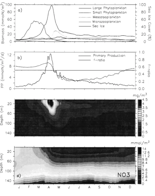
Figure 11-3. Domain-averaged seasonal cycle of the (a) depth-integrated (0-45 m) biomass of plankton components with sea ice cover percentage, (b) depth-integrated (0-45 m)
total primary production with the depth-averaged (0-45 m) f-ratio (ratio of the total new primary production over total primary production), (c) total Chi a and
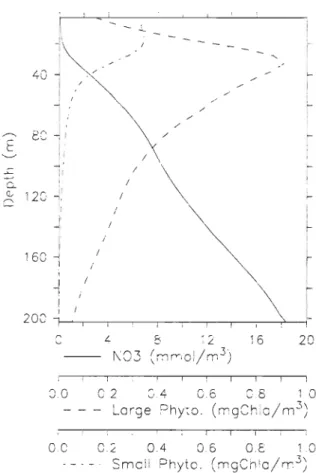
Figure ll-4. Vertical distribution of the domain-averaged concentrations of nitrate (solid line) , large phytoplankton (dashed line), and small phytoplankton (dashed-dotted line) on July l5th
... 27
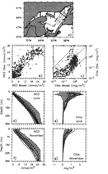
Figure ll-5. Comparisons of modeled and observed data: (a) sampling locations in June (circles) and November (crosses) 1997; scatter plot of (b) nitrate and (c) total Chi a; profiles of modeled (solid line) and observed (dashed line) concentrations of (d) nitrate and (e) total Chi a in June and of (f) nitrate and (g) total Chi a in November. The bold line represents the spatially-averaged profile. The shaded area is delimited by the spatially-averaged proflle ± standard deviation (thin
lines) ... 30
Figure ll-6. Mean seasonal cycle of total Chi a (integrated between 0-45 m) and sea ice
coyer percentage for the numerical domain and all subregions shown in Figure ll-1. The shaded area is delimited by the spatially-averaged time series of total Chi a (bold line) ± standard deviation (thin lines) ... 32
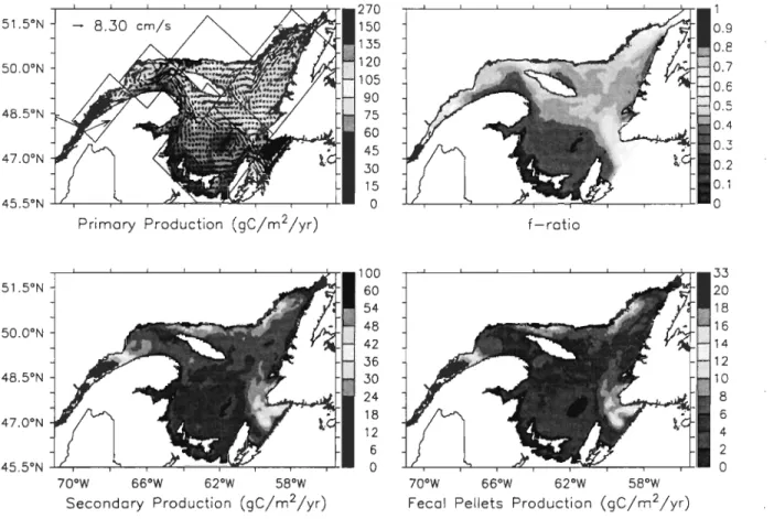
Figure ll-7. Regional overview of the depth-integrated (0-45 m) and yearly-cumulated total primary production with depth- and yearly-averaged (0-45 m) currents, depth- and yearly-averaged (0-45 m) f-ratio, depth-integrated (0-45 m) and yearly-cumulated total secondary production, and depth-integrated (0-45 m) and yearly-cumulated
fecal pellets production. Boxes on the upper left panel delirnit the studied subregions ... 34
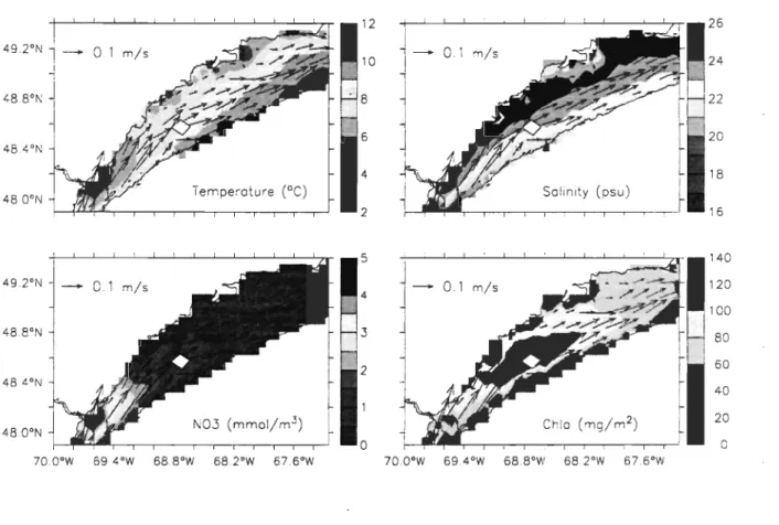
Figure 11-8. May to October mean in the LSLE of sea temperature (5 m), salinity (5 m), nitrate (5 m), and depth-integrated (0-45 m) total ChI a. Mean currents (5 m) are overlaid in all panels ... 36
Figure 11-9. Time series at a fixed station located in the upstream part of the LSLE (white
box in Figure 8) of the (a) total primary production (PP), (b) total Chl a with the depth of the nitracline overlaid, and (c) density (kg m-3) •.•••••••.•.•...•...••••••.•...••.•• 37
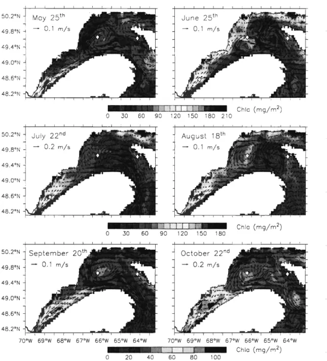
Figure 11-10. Snapshots of the depth-integrated (0-45 m) total Chi a (mg m-2) with depth-averaged (0-45 m) currents on May 25th, June 25th
, July 22od, August 18th, September 20th
, and October 22nd over the LSLE, NWG and northem
USt. ... 40
Figure II-Il. Time series at a fixed station located in the NWG (white box in Figure ll-lO) of the (a) total primary production (PP), (b) total Chl a with the depth of the nitracline overlaid, and (c) density (kg m-3). Vertical arrows at the top of each panel indicate each snapshot of Figure 11-10 ... 41
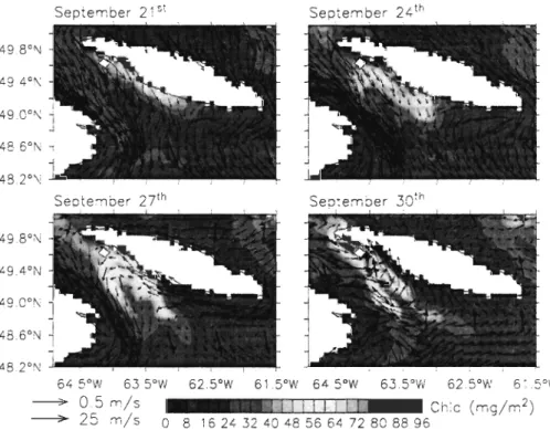
Figure TI-12. Snapshots of the depth-integrated (0-45 m) total Chl a with depth-averaged (0-45 m) currents and surface winds (bold arrows) on September 21sl
, September
24th, September 27th, and September 30th in the USt.. ....................... .43
Figure TI-13. Time series at a fixed station located in the USt (white box in Figure TI-12) of the (a) total primary production (PP), (b) surface winds, (c) total Chl a with the depth of the nitrac1ine overlaid, and (d) density (kg m-3). The two vertical lines delimit the time periods (September 21 sI to 30th) of the upwelling events shown in
Figure TI-I2 ... 44
Figure TI-I4. Snapshots of the total ChI a (5 m) with sea tempe rature contours (OC, 5 m) on September 27th, October 151, and October 5th• A 4 days (September 27th to
September 30th) Sea WIFS composite image is presented in the lower right
panel. ... 46
Figure TI-15. Time series at a fixed station located in the NEG (white box in Figure TI-14) of the (a) total primary production (PP), (b) total ChI a with the depth of the nitrac1ine overlaid, (c) nitrate concentration at 25 m, (d) temperature and salinity at 25 m, and (e) net water transport across the Strait of Belle-Isle with its moving window-averaged (14 days) equivalent overlaid. The two verticallines delimit the time periods (September 27th to October 5th) of the simulated events shown in
Figure ll-16. Vertical sections from the MS towards the Laurentian Channel illustrating the nitrate concentrations and NW-SE currents (m S-l) averaged over July-August.
The dashed and solid lines represent the seaward and north-westward current, respectively. On each panel, a solid line on a map indicates the location of the transect. ... 49
Figure ll-17. Time series of the depth-averaged (0-45 m) relative fraction of large phytoplankton (LP, bold solid line) averaged over the NWG, the NEG, and the MS. The shaded area is delimited by the mean ± standard deviation (thin solid lines). The horizontal dashed line indicates a relative fraction of 50 % ... 56
Figure Ill-l. Map of the Gulf of St. Lawrence and geographical appellations used in the paper. The bold lines indicate the boundaries of the 3-D coupled physical-biological model. ... 76
Figure ill-2. Scatter plot showing the linear relationship between salinity and the attenuation coefficient due to non-chlorophyllous matter (kp) derived from in situ
measurements. The linear regression gives the equation kp
=
-0.0364 Salinity+
1.1942 with a correlation coefficient ofr = 0.71. ... 79Figure ill-3. Positions of the (a) permanently moored thermometers, (b) sampling stations visited in 1998: AZMP croises in June (squares) and November (triangles), the fixed AZMP stations (circ1es), and the SeaWIFS validation croise in
October-November (rhombuses) ... 82
Figure ill-4. Comparisons of satellite-derived fields of SST and surface Chl a to simulated SST (5 m), Chl a (depth-averaged 0-10 m), and attenuation coefficient due to non-chlorophyllous matter (kp) for the June 7th-Il st period. The Mean simulated fields of surface wind and depth-averaged (0-10 m) current are overlaid on the Mean simulated SST and Chl a fields, respectively ...... 85
Figure ill-5. Same as Figure ill-4 for the July 2nd_8th period ... 86
Figure ill-6. Same as Figure ill-5 for the August 3rd_6th period ... 87
Figure ill-7. Same as Figure ill-6 for the August 28th-September 2nd period ... 88
Figure ill-8. Same as Figure ill-7 for the October 6th_14th period ... 89
Figure ill-9. Comparison of simulated SST with (a) AVHRR-derived SST and (b) in situ SST, and (c) comparison of in situ and simulated salinity. In situ data inc1ude measurements made in 1998 from the AZMP June and November cruises and
three flXed stations (see text). In panels (b) and (c), surface values are in red
whereas deeper values are in black (the whole water column) ... 90
Figure ID-lO. Comparisons of in situ SST to (a) simulated SST and (b) A VHRR-derived
SST ... 94
Figure ID-Il. Time series of hourly temperature records from permanently moored thermometers (in blue) compared to simulated temperature at the corresponding layer (in red). The number of the instrument (see Figure ID-3a) and the record depth appear on each panel. ... 96
Figure ID-12. Comparison of simulated ChI a with (a) SeaWIFS-derived ChI a and (b) in situ ChI a, and (c) comparison of in situ and simulated nitrate. In situ data include the whole set of available measurements made in 1998 (AZMP June and
November croises and fixed stations, SeaWIFS validation croise of October-November, see text). In panels (b) and (c), surface values are in red whereas
deeper values are in black (above 50 m for ChI a) the whole water column for
nitrate) ... 98
Figure ID-l3. Comparison of (a) simulated Chi a and (b) SeaWIFS-derived ChI a to in situ ChI a for the limited set of match-up points between Sea WIFS and in situ data ... 102
Figure IV-l. Annual mean of the depth-averaged (0-10 m) salinity (with currents overlaid) and
lep
for the ron using a variablelep ...
...
..
.
...
123Figure IV-2. Annual mean of the depth of the euphotic zone for the ron using a fixed or a variable lep ... 123
Figure IV -3. Yearly- and depth-integrated (0-45 m) new and regenerated primary production (PP) for the ron using a fixed or a variable.lep ... 125
Figure IV -4. Annual mean of the depth-averaged (0-10 m) nitrate and ammonium, and depth-integrated (0-10 m) total ChI a for the ron using a fixed or a variable
lep ...
.
...
.
...
..
...
.
...
.
....
.
126Figure IV -5. Annual mean of the depth-averaged (0-10 m) growth rates of large and small phytoplankton (LP and SP, respectively) for the ron using a fixed or a variable lep.
Because the two phytoplankton groups show the same response to light, only one panel is presented for both size classes ... 127
Figure IV -6. Mean seasonal cycle of total ChI a (integrated between 0-45 m) and sea ice
cited in the text. The black and red lines correspond to the ron using a fixed and variable kp, respectively ... 129
Figure IV-7. Time series of the vertical distribution kp (m-I). The nutricline from the run
using a fixed
kp
(black dashed line) and a variable kp (black line) are overlaid ... 131Figure IV -8. Map of the Estuary and Gulf of St. Lawrence. Acronyms indicate the subregions cited in the text. The bold lines are the open boundaries of the cou pied mode!. The thin lines indicate the transects used for nitrogen fluxes estimations. Circles show the location of the Gaspé (nearshore) and Anticosti (offshore) stations ... 133
Figure IV-9. Figure IV-9. Ratios between simulated depth-integrated (0-30 m) vs in situ depth-integrated (0-30 m) nitrate concentrations at the a) Gaspé and b) Anticosti stations. The black and red circles correspond to the ron using a fixed and variable
lep,
respectively; time series of the c) depth-integrated (0-30 m) nitrate flux from the LSLE with a fixed kp (in black) and variable kp (in red) and d) depth-averaged(0-30 m)
kp
at the Gaspé (black line) and Anticosti (black dashed line) stations ... 136LISTE DES TABLEAUX
Table II-l. State variables and partial equations ... 20
Table II-2. Parameters used in the ecosystem model.. ... 21
Table ill-l. Time periods and number of images used to build the A VHRR and Sea WIFS
composites ... 81
Table ill-2. Root mean square (RMS, OC) error and mean relative difference (MRD, %) calculated between the A VHRR-derived and simulated SST (n=50237).
Coincident points for each time period are shown in parentheses ... 92
Table ill-3. Root mean square (RMS) error and mean relative difference (MRD, %) calculated between the in situ (bottle measurements) and simulated temperature, salinity, nitrate and ChI a. Numbers of sampling are shown in parentheses ... 92
Table illA. Root mean square (RMS, OC) error and mean relative difference (MRD, %) calculated between the in situ (moored thermometers) and simulated or A VHRR-derived SST (n = 42). Coincident points for each time period are shown in parentheses ... 95
Table III-5. Root mean square (RMS, mg Chi a m-3) error and mean relative difference (MRD, %) calculated between the Sea WIFS-derived and simulated Chi a concentrations (n=48361). Coincident points for each time period are shown in parentheses ... 99
Table ID-6. Root mean square (RMS, mg Chl a m-3) error and mean relative difference (MRD, %) calculated between the in situ and simulated or SeaWIFS-derived ChI a concentrations for the GSL subregions (n=35). The number of match-up points for each subregion is displayed in parentheses ... 103
Table IV-l. Mean annual primary production of the GSL and its subregions (g C m-2 yr
-1 ) ........................ 130
Table IV -2. Ratio of the and depth-integrated (0-30 m) nitrate flux over the yearly-and depth-integrated (0-30 m) organic nitrogen flux ... 135
Table IV-3. Mean nitrate flux (0-30 m) in summer (in IOmol S-I). Percentages in parentheses indicate the bias between the fluxes simulated using a fixed or a salinity-dependant lep and those provided by Savenkoff et al. [2001] ... 139
De par sa proximité et sa dynamique, le golfe du Saint-Laurent (GSL) est un bassin expérimental unique pour l'étude des interactions physiquelbiologie à méso-échelle. Une des plus grandes mers intérieures semi-fermée, le GSL fait la connexion entre les Grands Lacs, le fleuve Saint-Laurent et l'océan Atlantique Nord. Les eaux de surface estuariennes sont évacuées du GSL par le détroit de Cabot, alors que les eaux salées de l'océan Atlantique et de la mer du Labrador y pénètrent principalement par les détroits de Cabot et de Belle-Isle, respectivement. Les variations saisonnières des débits d'eau douce du fleuve Saint-Laurent et de la rivière Saguenay contribuent grandement au patron de circulation des eaux de surface estuariennes vers le GSL. La couverture saisonnière de glace de mer associée au climat sub-arctique s'étend de janvier à avril et atteint la limite des glaces de mer la plus au sud de l'hémisphère Nord. Les marées sont modérées à fortes et la variabilité du régime des vents très synoptique. Ces forçages hydrologiques, océaniques et atmosphériques, associés aux dimensions du golfe (226000 km2, 150 m de profondeur
moyenne), génèrent une circulation complexe où les tourbillons, les résurgences côtières et les zones frontales se superposent à une circulation de type estuarienne [Koutitonsky et Budgen, 1991; Fuentes-Yaco et al., 1995; 1996; 1 997ab; Saucier et al., 2003]. Cette dynamique à méso-échelle pourrait jouer un rôle important dans la dynamique de l'écosystème planctonique du Saint-Laurent. de Lafontaine et al. [1991] soulignent une certaine hétérogénéité spatiale dans le GSL illustrée par des différences dans le cycle saisonnier, la composition spécifique et la structure de taille du phytoplancton et du
zooplancton, et probablement par des réseaux trophiques différents. Les images satellites de température de surface (http://www.osl.gc.calteledetection/fr/index.html) et de couleur de l'eau [Fuentes-Yaco et al., 1995; 1997a] suggèrent une forte variabilité hydrodynamique à méso-échelle dans le GSL, particulièrement au printemps et en automne, soit pendant les périodes de plus forte production. Des observations récentes confIrment que la variabilité interannuelle des propriétés des masses d'eau du GSL [Saucier et al., 2003], de la biomasse planctonique dans l'estuaire maritime du Saint-Laurent [EMSL; Starr et Harvey, 2000; Starr et al., 2001], du recrutement des stocks de poisson [Runge et al., 1999], des patrons d'agrégations du krill et des baleines à la tête du chenallaurentien [Simard et Lavoie, 1999; Lavoie et al., 2000] est fortement liée à l'influence du climat et des apports d'eau douce sur les processus de mélange et la circulation.
TI apparaît nécessaire d'engager un plus grand nombre d'études afIn de comprendre, quantifier et, éventuellement prédire, les effets de la variabilité des processus physiques sur la production planctonique marine. C'est de l'échelle locale (1-10 km) à moyenne
(10-plusieurs centaines de km) que les interactions directes entre la dynamique des écoulements océaniques et la production des communautés planctoniques sont les plus importantes [Garçon et al., 2001; Lévy et al., 2001]. En effet, la dynamique de ces écoulements océaniques d'échelle locale à moyenne obéit à des échelles de temps caractéristiques (du jour à quelques mois), proches de celles des processus biologiques impliqués dans la production planctonique (de la journée pour la production primaire à quelques semaines pour la production secondaire). Ces structures de méso-échelle constituent une fraction importante de l'énergie cinétique des océans [Le Traon, 1991] et se singularisent par leur
dynamique dans l'espace et dans le temps. L'activité biogéochimique à l'échelle de ces structures est en étroite relation avec cet aspect dynamique. Les structures de méso-échelle sont impliquées dans l'enrichissement de la couche de surface en sels nutritifs via un
transport horizontal [Williams et Follows, 1998] et vertical [Martin et Richards, 2001]. McGillicuddy et al. [1998] suggèrent que le déséquilibre entre les estimations de production
primaire et la disponibilité en sels nutritifs dans les eaux oligotrophes de la mer des Sargasses pourrait être compensé par les apports verticaux de sels nutritifs au centre des tourbillons cycloniques de méso-échelle. Ces apports peuvent être équivalents à ceux engendrés par la convection hivernale de la colonne d'eau [Siegel et al., 1999]. La
dynamique de l'écosystème planctonique pélagique en zone frontale est également fortement liée aux processus de résurgence et de subduction des masses d'eau. Ces mouvements verticaux peuvent contribuer à augmenter la production primaire dans la zone euphotique tout en générant une hétérogénéité spatiale de cette production et de la biomasse phytoplanctonique [Spall et Richards, 2000] qui peuvent être découplés à l'échelle locale
[Zakardjian et Prieur, 1998]. La plus forte production générée par cette dynamique frontale
modifie la relation taille/abondance des cellules phytoplanctoniques et donc la structure trophique des communautés [Rodriguez et al., 2001]. La variabilité de la structure et de la
productivité de l'écosystème planctonique en zone frontale peut mener à des fluctuations de l'exportation de carbone vers les couches profondes [Claustre et al., 1994; Peinert et Miquel, 1994; Rodriguez et al., 2001]. Les flux de carbone sont donc fortement liés à la
dynamique de méso-échelle. L'impact de cette dynamique sur la biogéochimie de la colonne d'eau est local mais peut s'étendre à l'échelle des bassins océaniques [Lorentz et al.,
1993; Claustre et al., 1994; McGillicuddy, 2001]. Cette variabilité à méso-échelle n'est pas typiquement résolue dans les modèles de circulation à l'échelle globale [Doney et al., 2001] mais les modèles de circulation à plus haute résolution apportent l'évidence qu'elle est fondamentale pour l'estimation de la productivité primaire et l'exportation de matière organique [Mahadevan et Archer, 2000; Doney et al., 2001; Lévy et al., 2001; McGillicuddy, 2001]. L'échelle temporelle associée à ces structures de méso-échelle dans l'océan ouvert est de quelques semaines à plusieurs mois. En milieu oligotrophe, comme dans la région du Gulf Stream, l'enrichissement en nitrate de la zone euphotique lié à la cinétique de tourbillons cycloniques est un processus clé pour la productivité du système. La durée de vie des structures de méso-échelle en milieu côtier est généralement plus courte, de quelques jours à plusieurs semaines, et ces dernières répondent à des forçages fortement synoptiques. À l'échelle régionale et locale, cette activité a des implications majeures sur la distribution spatiale du phytoplancton [Pavelson et al., 1999], la production primaire [Morân et al., 2001] et la structure des communautés planctonique [Ressler et Jochens, 2003].
Dans le Saint-Laurent, les structures de méso-échelle ont été principalement documentées dans l'EMSL et dans le nord-ouest du golfe. Dans l'EMSL, le fort hydrodynamisme lié aux apports saisonniers d'eau douce du fleuve Saint-Laurent influence fortement la distribution spatiale et temporelle du phytoplancton [Therriault et Levasseur, 1985]. Le patron de la circulation estuarienne dans l'EMSL se caractérise par la formation d'instabilités et de tourbillons [Gratton et al., 1988; Ingram et EI-Sabh, 1990; Mertz et Gratton, 1990] liée aux dimensions de l'EMSL. En effet, la largeur de l'EMSL peut
atteindre 50 km soit plusieurs rayons internes de Rossby (10 km; Mertz et al., 1988),
échelle caractéristique des mouvements baroclines. En dépit de conditions environnementales favorables (stratification, lumière, sels nutritifs), le déclenchement de la floraison phytoplanctonique dans l'EMSL a lieu deux mois plus tard [fin juin-début juillet; Levasseur et al., 1984; Roy et al., 1996] que dans le GSL [avril-mai; Sévigny et al., 1979], soit en période de plus faible deôit fluvial [Therriault et al., 1986]. La communauté
phytoplanctonique est largement dominée en été par les diatomées, les flagellés étant présents tout au long de l'année quoique plus abondants en juillet et septembre [Roy et al., 1996; Levasseur et al., 1984; Savenkoff et al., 1998]. Ce schéma est atypique comparé aux eaux côtières de même latitude. Bien que les causes de la floraison tardive dans l'EMSL ne soient pas encore bien établies, la circulation des eaux estuariennes de surface est probablement un facteur majeur agissant de concert avec d'autres facteurs environnementaux tels que le régime de mélange turbulent, la turbidité de la colonne d'eau et la sédimentation des cellules phytoplanctoniques [Therriault et Levasseur, 1985; Zakardjian et al., 2000]. Dans le cadre du programme COUPPB (COUplage des Processus Physiques et Biogéochimiques), Gratton et V ézina [1994] ont mis en évidence la formation de fronts de densité transitoires (3-5 jours) dans l'axe transversal de l'EMSL liée au passage de pulses d'eau douce en provenance de l'amont de l'estuaire. Vézina et al. [1995] ont montré que le déclenchement de la floraison estivale au large de Rimouski coïncidait avec la formation d'un tel front. À ce forçage s'ajoute l'effet du cycle de marée
vive-eau/morte-eau sur le cycle de production primaire, phénomène dont l'importance dans l'EMSL a déjà été soulignée [Sinclair, 1978; Legendre et Demers, 1985]. Le fait que les concentrations en
sels nutritifs dans l'EMSL soient généralement élevées tout au long de l'année [Levasseur et al., 1984] supporte d'autant plus l'hypothèse que le cycle de production primaire soit
principalement sous le contrôle de la dynamique de la circulation de méso-échelle, du cycle de marée et de la disponibilité en lumière.
Dans le nord-ouest du golfe, les deux structures majeures de la circulation sont le courant de Gaspé et le tourbillon d'Anticosti. Le courant de Gaspé est un courant côtier barocline principalement alimenté par l'écoulement des eaux de surface estuariennes. La
dynamique du courant de Gaspé montre une variabilité synoptique importante [Koutitonsky et Budgen, 1991] illustrée par le développement de méandres et de tourbillons [Sheng,
2001] et par l'écartement de la rive sud de ce courant dessalé. Le tourbillon d'Anticosti, cyclonique et quasi-permanent [El Sabh, 1976; Koutitonsky et Budgen, 1991], est séparé du
courant de Gaspé par un front de densité [Tang, 1980a]. Le fort gradient de vitesse et de
densité entre le tourbillon d'Anticosti et le courant de Gaspé est à l'origine d'une circulation trans-frontale [Tang, 1980a] qui constitue une connexion entre ces deux structures
hydrodynamiques. Les instabilités du courant de Gaspé peuvent aussi affecter une grande partie du nord-ouest du golfe et interagir directement avec le tourbillon. Cette dynamique de la circulation affecte l'écosystème planctonique du système tourbillon d'Anticosti/courant de Gaspé. Typiquement, les concentrations estivales en sels nutritifs dans le tourbillon sont limitantes pour la croissance des diatomées et, ainsi, l'écosystème pélagique est principalement dominé au cours de l'été par les flagellés et dinoflagellés lesquels peuvent constituer plus de 80 % de la biomasse phytoplanctonique [Sévigny et al.,
phytoplanctonique du courant de Gaspé est généralement dominée par les diatomées bien qu'accompagnées de petits flagellés abondants [Levasseur et al., 1992]. Levasseur et al. [1992] ont rapporté un transport de la biomasse phytoplanctonique produite dans le courant de Gaspé vers le tourbillon d'Anticosti. Quand l'écoulement des eaux de surface estuariennes est important, la biomasse phytoplanctonique à la surface du courant de Gaspé semble être transportée par mélange turbulent au-delà du front et diluée dans les eaux de surface du tourbillon [Levasseur et al., 1992]. En revanche, quand l'écoulement s'atténue (fm juillet) la biomasse phytoplanctonique, constituée principalement de diatomées, semble s'accumuler dans le front et à la base du courant [Sévigny et al., 1979; Levasseur et al.,
1992]. De plus, Plourde et Runge [1993] suggèrent qu'une partie de la biomasse zooplanctonique du tourbillon n'ait pas une origine locale mais estuarienne [e.g., Vézina et al., 2000]. Le tourbillon d'Anticosti n'est donc pas une structure hydrodynamique isolée mais sa dynamique est au contraire influencée par la dynamique de méso-échelle de la circulation estuarienne.
Un troisième type de structure, plus faiblement documenté, est lié aux résurgences d'eau froide régulièrement observées dans le nord du golfe, sur la Basse Côte Nord [Koutitonsky et Budgen, 1991] et à l'extrémité ouest du détroit Jacques Cartier où le mélange tidal entre les eaux intermédiaires et les eaux de surface est intense [Pingree et Griffiths, 1980]. Au sud de l'île d'Anticosti, ces résurgences d'eau côtière sont plus probablement générées par les vents de nord-ouest ou le mélange tidal [Koutitonsky et Budgen, 1991]. Les images satellites de température de surface indiquent la présence de résurgences d'eau froide dans cette zone en été comme en automne
(http://www.osl.gc.ca/teledetectionlfrlindex.htmI). Ce type de résurgences est généralement associé à une plus forte production primaire liée à l'apport en surface d'eau intermédiaire riche en sels nutritifs. La côte sud de l'île d'Anticosti n'ayant jamais fait l'objet de programme d'échantillonnage, aucune donnée concernant la production planctonique n'est actuellement disponible. Toutefois, des estimations de concentration de chlorophylle a obtenues à l'aide d'images du capteur CZCS (Coastal Zone Color Scanner) ont permis à Fuentes-Yaco et al. [1995; 1997ab] de mettre en évidence des épisodes de plus forte biomasse phytoplanctonique sur la rive sud de l'île d'Anticosti. Certaines images satellites
de couleur de l'eau montrent des filaments riches en chlorophylle a qui partent de la zone de plus forte biomasse et envahissent le 'nord du plateau madelinien. Ces structures laissent supposer qu'une fraction de la biomasse phytoplanctonique produite dans la zone de résurgence au sud d'Anticosti pourrait être exportée via la circulation à méso-échelle vers le reste du GSL [Fuentes-Yaco et al., 1995; 1996].
Au regard de cette revue de littérature non-exhaustive sur le couplage physique-biologie à méso-échelle, le GSL se pose comme un système complexe et riche en processus susceptibles d'influencer le cycle annuel de production planctonique. L'objectif général de la thèse est de quantifier l'effet de cette circulation à méso-échelle sur la dynamique de la production planctonique du Saint-Laurent. Pour atteindre cet objectif, le premier modèle d'écosystème planctonique couplé au modèle prognostique de circulation du GSL [e.g., Saucier et al., 2003] a été developpé au cours de cette thèse afin de pleinement capturer la variabilité du système. L'atout majeur de cette approche réside dans la possibilité d'atteindre la résolution temporelle, tidale à saisonnière, caractéristique des processus
hydrodynamiques du Saint-Laurent. Trois objectifs spécifiques sont fixés afin de répondre à l'objectif général. Le premier objectif spécifique (chapitre II) consiste à vérifier la robustesse écologique du modèle couplé physique-biologie à l'échelle régionale et à décrire qualitativement et quantitativement la variabilité sous-régionale du cycle saisonnier planctonique en réponse à des régimes hydrodynamiques variés qui caractérisent le système. Les observations in situ seules peuvent difficilement rendre compte de l'effet de la variabilité à méso-échelle sur la dynamique du phytoplancton. En revanche, les données satellites de température de surface et de couleur de l'eau y contribuent en apportant une information à haute résolution temporelle Gusqu'à quelques heures) et spatiale (jusqu'à un kilomètre). Le second objectif spécifique (chapitre ID) vise ainsi à valider les solutions du modèle couplé à l'échelle régionale et synoptique à l'aide de données satellites de température de surface (advanced very high resolution radiometer) et de couleur de l'eau (Sea-viewing Wide Field-of-view Sensor). Le troisième et dernier objectif spécifique de la thèse (chapitre IV) se place dans la continuité des résultats obtenus dans le troisième chapitre, notamment en ce qui concerne l'importance des eaux turbides estuariennes dans le Saint-Laurent. TI vise à quantifier l'impact de la turbidité des eaux continentales, particulièrement du panache estuarien, sur la dynamique planctonique du GSL.
Le corps de cette thèse est constitué de trois chapitres rédigés en anglais sous forme d'articles scientifiques ainsi que d'une introduction et conclusion générale en français. Le second chapitre est publié dans la revue Journal of Geophysical Research (Ocean). Le troisième chapitre est en révision après soumission à la revue Journal of Marine Systems. Le quatrième chapitre sera soumis à une revue internationale pour publication.
II. SEASONAL VERSUS SYNOPTIC V ARIABILITY IN
PLANKTONIC PRODUCTION IN A IDGH-LATITUDE MARGINAL
ABSTRACT
The Gulf of St. Lawrence (Canada) is a subarctic marginal sea characterized by highly variable hydrodynamic conditions that generate a spatial heterogeneity in the marine production. A better understanding of physical-biologicallinkages is needed to improve our ability to evaluate the effects of climate variability and change on the gulf' s planktonic production. We develop a three-dimensionnal (3-D) eddy-permitting resolution physical-biological coupled model of plankton dynamics in the Gulf of St. Lawrence. The planktonic ecosystem model accounts for the competition between simplified herbivorous and microbial food webs that characterize bloom and post-bloom conditions, respectively, as generally observed in temperate and subarctic coastal waters. It is driven by a fully prognostic 3-D sea ice-ocean model with realistic tidaI, atmospheric and hydrological forcing. The simulation shows a consistent seasonal primary production cycle, and highlights the importance of local sea ice dynamics for the timing of the vernal bloom and the strong influence of the mesoscale circulation on planktonic production patterns at subregional scales.
INTRODUCTION
General circulation models generally predict that global climate change associated with increased greenhouse gas concentrations in the atmosphere will lead to an amplified warming in the Arctic and its adjacent seas over the next century (5-8°C in 2070; e.g., Hol/and and Bitz, 2003). Among those, the Gulf of St. Lawrence (GSL) is a large semi-enclosed sea of 226000 km2 that connects the Great Lakes and the St. Lawrence River with the North Atlantic Ocean [e.g., Koutitonsky and Budgen, 1991]. Runoff from the St. Lawrence watershed is the second most important source of freshwater from North America into the North Atlantic Ocean [e.g., Bourgault and Koutitonsky, 1999]. The GSL exhibits a subarctic climate with a seasonal sea ice cover present between J anuary and April, and sheds the southernmost extent of sea ice in the northern hemisphere. Freshwater runoff, large to moderate tides, and highly synoptic winds drive the gulfs circulation. These physical forcing, coupled with the relatively large dimensions of the gulf (several internal Rossby deformation radii) and an average depth of 150 m, generate a complex hydrodynamics with eddies, coastal upwellings, and fronts superimposed on a mean estuarine-like circulation [e.g., Koutitonsky and Bugden, 1991; Saucier et al., 2003]. These hydrodynamic conditions have been shown to have a marked effect on summer primary production in the northwestern Gulf [Levasseur et al., 1992; Fuentes-Yaco et al., 1995, 1996, 1997ab; Tremblay et al., 1997], and are thought to generate a spatial heterogeneity in the marine production of the GSL [e.g., de Lafontaine et al., 1991]. Savenkoff et al. [2001] also suggest that the GSL can be subdivided into distinct subregions on the basis of specific
hydrodynamic regimes that affect the nutrient transport and the resulting planktonic production. Recent observations confmn that the high interannual variability in plankton biomass in the Lower Estuary [Starr and Harvey, 2000; Starr, 2001], the recruitment of fish stocks in the southem gulf [Runge et al., 1999], the aggregation of krill and whales at the head of the Laurentian Channel [Simard and Lavoie, 1999; Lavoie et al., 2000], and the water masses properties of the GSL [Saucier et al., 2003] are strongly linked to the influence of climate and freshwater inputs on the mixing and circulation processes. However, it has not yet been possible to quantify together the detailed circulation and the response of the planktonic ecosystem.
Prior to any attempt to predict the effects of global climate variability and changes on the GSL system, we must first acquire a better knowledge of the links between the physical environment and the short-term to interannual variations in planktonic production. In order
to improve our capability to predict these responses, we need to develop models that reproduce the spatio-temporal variability of the primary and secondary production cycles. Modelling of planktonic production in the St. Lawrence marine system has been limited to
one-dimensionnal (l-D) models of the carbon cycle in the northwestem [Tian et al., 2000] and northeastem [Tian et al., 2001] GSL, to a 2-D modelling study of the phytoplankton production in the Lower Estuary [Zakardjian et al., 2000], and to 3-D modelling of copepods population dynamics [Zakardjian et al., 2003]. This paper aims at describing and quantifying the circulation-planktonic production coupling in the GSL using a detailed 3-D physical-biological model. The coupled model includes both simplified herbivorous and microbial food webs typical of bloom and post-bloom conditions respectively, as generally
observed in temperate and subarctic coastal waters. It is driven by a 3-D high resolution primitive equations ocean-sea ice regional model [Saucier et al., 2003] with realistic tidal, atmospheric and hydrologic forcing.
In the present paper, we focus on the ecological robustness of the coupled model
performances al the regional scale and the subregional variability of the seasonal plankton cycle in response to varied hydrodynamic conditions. These first results demonstrate that the coupled model predicts realistic levels of biomass and a seasonal cycle of planktonic production dominated by the spring phytoplankton bloom, as observed in the GSL. In
addition, the model generates a large synoptic and spatial variability in planktonic production in response to the buoyancy-driven circulation, tidal mixing, and wind events. As a consequence, primary production can locally be as important as during the spring bloom.
MODEL FORMULATION
1. The 3-D regional circulation model
A detailed description of the deterministic sea ice-ocean coupled model is presented in Saucier et al. [2003], and the characteristics are briefly reviewed here. The ocean model is govemed by the shallow water equations solved by a finite difference scheme. It incorporates a level2.5 turbulent kinetic energy equation [Mellor and Yamada, 1974, 1982] and diagnostic master length scales. A thermodynamic and dynamic sea ice model [Semtner, 1976; Flato, 1993] is coupled with the ocean mode!. Bulk aerodynamic exchange formulas govem the heat and momentum fluxes between the ocean, sea ice and atmosphere. The model domain covers the Estuary and the Gulf of St. Lawrence and is delimited by three open boundaries at the Cabot Strait, the Strait of Belle-Isle, and the upper limit of the tidal influence near Montreal (Figure ll-l). The grid resolution is 5 km on the horizontal
and ranges from 5 to 20 m in the vertical, with free surface and bottom layers adjusted to topography. The model is fully deterministic and tracer conserving [e.g., Saucier et al., 2003], driven by a detailed atmospheric forcing (three-hourly winds, light, precipitation),
daily river ronoff data from the St. Lawrence river and the 28 most important tributaries, hourly water levels (co-oscillating tides) and monthly mean temperature and salinity profiles at the Strait of Belle-Isle and Cabot Strait. The model accounts for the variations of sea ice, tides, momentum, heat and salt fluxes, and river discharges with a time step of 300 s and reproduces the high frequency to interannual variations of the circulation, water mass properties, and sea ice coyer. Simulations for 1996-1997 [Saucier et al., 2003] and recently
52DN
~
~
tfelle-isie i"
, rt1 1 ! 58°WFigure 11-1. Map of the Estuary and Gulf of St. Lawrence. Bold lines delimit the numerical domain. Boxes indicate the studied subregions: Lower Estuary of St. Lawrence (LSLE), northwestem Gulf of St. Lawrence (NWG) , Unguedo Strait (USt), Magdalen Shallow (MS), southem Laurentian Channel (SLC), northeastem Gulf of St. Lawrence (NEG) and Jacques Cartier Strait (JCS).
through 2003 [Saucier et al., 2005, in prep.] have been successfully compared to temperature and salinity data, the sea ice cover, water levels, and past analyses of transport in the Lower Estuary and GSL. In particular, the model reproduces the main well-known circulation features and their seasonal variations. Those include the year-round cyclonic gyre over the northwestern GSL known as the Anticosti Gyre, the Gaspé CUITent, an unstable buoyancy-driven baroclinic coastal jet, and the southeastward outflow through western Cabot Strait.
2. The planktonic ecosystem model
The planktonic ecosystem model (Figure II-2) was developed in a moderately complex way in order to limit the number of transfer functions and parameters, and to allow an easier interpretation of the biological response to the high frequency to seasonal variations of environmental conditions generated by the physical model. Primary producers are size-fractionated into large (>5 ~m) and small (<.5 ~m) phytoplankton (LP and SP,
respectively) both growing on nitrate (N03) and ammonium (NH4). Similarly, the secondary producers are divided in mesozooplankton (200-2000 ~m, MEZ) and
microzooplankton (20-200 ~m, MIZ). Two detrital compartments close the cycling of nitrogen, namely particulate and dissolved organic nitrogen (pON and DON, respectively). A close coupling between small phytoplankton and microzooplankton dynamics, autochthonous nitrogen release and DON ammonification is assumed to represent the dynamic of the microbial food web. State variables and partial differential equations are listed in Table II-l and detailed in the Appendix, and parameters definition and values are
r ---.
,
\~-1--~---~----
,
(~
NH4 I4j- - - - { --- - _ /~----Figure ll-2. Conceptual planktonic ecosystem model including nitrate (N03), ammonium
(NH4) , large phytoplankton (LP) , small phytoplankton (SP), mesozooplankton (MEZ),
microzooplankton (MIZ) , particulate organic nitrogen (PON) and dissolved organic nitrogen (DON). Arrows represent nitrogen fluxes between the biological components.
given in Table 11-2.
3. Coupling with the 3-D regional circulation model
The partial differential equation used to compute the evolution of a simulated scalar (here C) is of the form:
where t is time, x, y, z are the spatial coordinates, u, v, w are the CUITent velocities in the x, y, z directions, respectively; Kx, Ky and Kz are the horizontal and vertical eddy diffusion coefficients, respectively; the sinks and sources are described in Table 11-1. At each time step, the transport of each biological variable is performed by the advection-diffusion routine of the physical model while the sink and source terms are explicitly computed afterwards.
The present simulation covers the 1997 one year period. This year was chosen because the atmospheric and runoff conditions were close to their respective climatology. The physical and biological models are initialized with observations acquired during November and December 1996 throughout the GSL from the Atlantic Zone Monitoring Program [AZMP; Therriault et al., 1998]. In order to initialize the biological model with a dynamically balanced physical ocean, the circulation model starts in November 1996 with observed temperature-salinity profiles interpolated to each model layer. It runs until January Ist 1997 at which time the profiles of nitrate and chIorophyll
Table 11-1. State variables and partial equations Symbol Meaning N03 Nitrate NH4 Ammonium LP Large phytoplankton SP Small phytoplankton MEZ Mesozooplankton MIZ Microzooplankton
paN Particulate organic nitrogen
DON Dissolved organic nitrogen
dN03
- - = -~LP .NuN03LP .LP - ~ sp.NuN03sp .SP
dt
dNH4- - = -~LP .NuNH4LP .LP - ~sp·NuNH4sp .SP + ex.MEZ + gzMIZ .(1-eg).(1- assMlZ ).MlZ
dt
+reffi.DON
dLP ( LP ) dLP
- - = (~LP - ffiLP ).LP - gZMEZ' .MEZ - sedLP' ~
dt
LP+MIZ uZdSP
- - = (~sP - ffisp ).SP - gZMlZ'MlZ
dt
dMEZ 2
- - - = gzMEZ .assMEZ .MEZ - ffiMEZ.MEZ - ex.MEZ
dt
dMIZ ( MIZ )
- - = gzMlZ .assMlZ .MIZ - ffiMlZ .MIZ - gzMEZ' .MEZ
dt
LP+MIZdPON dPON
- - = gZMEZ·(I-assMEZ)·MEZ-ffiLP·LP-fg.PON -sedPON" :\
dt
uZdDON
- - - = gZMlZ .eg. (1 - assMlZ ).MIZ + ffiMlZ .MIZ + ffiMlZ .MIZ - rem. DON
dt
Table 11-2. Parameters used in the ecosystem model Symbol - -_ .-Light field kw ~
Meaoing Value and unit
Pure seawater attenuation coefficient 0.04 m-I
Nonchlorophyllous matter-associated attenuation coefficient 0.04 m-I
--- ---Phytoplankton
k3LP LP half-saturation constant for N03 uptake 1 mmol N m-3
k4LP LP half-saturation constant for NH4 uptake 0.5 mmol N m-3
k3sp SP half-saturation constant for N03 uptake 1 mmol N m-3
k4sp SP half-saturation constant for NH4 uptake 0.1 mmol N m-3
ke LP and SP half-saturation constant for light use 10 Ein m-2 d-I
dtmin LP and SP minimum doubling time 0.5 d
mLP.SP LP and SP mortality 0.02d-1
sedLP LP sinking rate 1 md-I
Reference
Morel [1988]
fitted
Parsons et aL [1984]
Kiefer and Mitchell [1983]
Zakardjian et al. [2000] fitted Smayda [1970] _._---_._---,---_._--_._---_._---_.-•. __ ...
__
._---_ .. _--_.,--_.- --._---_._ ..__
._-_
.. _ ...__
..._
... -. '._--- -. __ .. _ ... _-... _ .,-_._. Zooplankton gmaxMEZ gmaxMIZ iVMEZ kMIZ assMEZ assMIZ mMEZMEZ maximum grazing rate MIZ maximum grazing rate
Ivlev parameter of MEZ grazing formulation half-saturation constant for MIZ grazing MEZ assimilation efficiency
MIZ growth efficiency MEZ mortality 0-2 d-I 2 d-I 0.8 (mmol N m-3
r
l 0.8 mmol N m-3 70% 30% 0.05 (mmol N m-3 d-1rl fitted Strom et al. [200 1] Frost [1972] fitted Kjorb~e et aL [1985] Riegman et al. [1993] fittedmMIZ MIZ mortality 0002 dol fitted
ex NH4 excretion by MEZ 0005 dol Sa(z and A Ica raz [1992]
eg DON egestion by MIZ 30% Lehrter et al. [1999]
Detritus
sedPON PON sinking rate 100 mdol Turner [2002]
fg PON fragmentation rate 0005 dol Fasham et alo [1990]
November-December 1996 observations are in tum interpolated and merged into the simulation. Equal concentrations of large and small phytoplankton were assumed to initiate the run. Because of the lack of data for the remaining biological scalars for the same period, idealized profiles were used. Values of 1 mmol m-3 for ammonium [e.g., Levasseur et al., 1990; Tremblay et al., 2000; Zakardjian et al., 2000], 0.05 mmol m-3 for DON and 0.005
mmol m-3 for PON were assigned to each depth interval from the surface to the last active
layer. Concentrations for mesozooplankton and microzooplankton were set to 0.4 mmol N m-3 [e.g., Sime-Ngando et al., 1995; Roy et al., 2000; Savenkoff et al., 2000] in the upper 25
m and to 0 below this depth. Laterally homogenous initial conditions for the biological sca1ars were assigned to each grid point. At the open boundaries of the domain, the concentrations are maintained constant through time and are the same than those used for the initial conditions. Both chemical and biological variables are set to zero in the inflowing rivers. A dynamic equilibrium is reached after two to three weeks in January, mostly affecting the mesozooplankton and nitrate fields (seen in Figure ll-3ac). Sea ice and winter mixing maintain the biological variables in a slowly-varying state until the spring bloom onset.
~E 1 00 +! ----'--~--'-___,,_-'----'----'---.L.--L---'--l.----'--_+_r 1 00 (/) -1 ) - -Large Phytoplanktor.
r
"~o 80
j
a
- -s
mali Phytopiankton r LL 80 mOnE 60 ~ - - - Mesozoopiankton L~ 60 ~
E - -Microzoopiankton ~ , ,
~
40j
--
Sea Ice 40~
Ë
20 ~ 20 ;:, o ~ iii 0 ... ---.. --- --- 0 '-" ---. 12J
f' 1.0 ~ ' 1 b) Primary Production N ~ f-ratio 0.8 -( 8 zJ
'____
06 . 1 o !---+--~---~~~r 0ê
4~
l
tf- 0.46
0.2 0.. 0.. 0 +I--.-~-~-~-~-~-~-~~-~-~-_+! 0.0 20 ---. E '-" 60 .r ~ Q. Q) o 100 140 20 ---. E 60 .r ~ Q. ~ 100 140 J F M A M J J A s o N mg/m3 , 4.5 mmol/m3 14 12.6 11.2 9.8 8.4 7 5.6 42 2.8 1.4 o oFigure 11-3, Domain-averaged seasonal cycle of the (a) depth-integrated (0-45 m) biomass of plankton components with sea ice cover, (b) depth-integrated (0-45 m) total primary production with the depth-averaged (0-45 m) f-ratio (ratio of the total new primary production over total primary production), (c) total ChI a and (d) nitrate. The horizontal line in panel b indicates a f-ratio of 0.5.
RESULTS
J. Mean seasonal biomass and production cycle
The coupled model produces a strong spatial and temporal variability of planktonic production due to the sea ice dynamics, freshwater runoff, tidal and wind-induced circulation and mixing. In order to facilitate the interpretation of the model results we examine the domain-averaged time series over the simulation period (Figure 11-3). After a relatively low production winter period due to low light intensity and the sea ice coyer (January to March), the diatom-dominated vernal bloom occurs in the second half of April following sea ice melt (Figure 11-3a), and increasing light levels and stratification. The simulated timing of the bloom is consistent with previous observations, occurring generally from the end of March to the end of April [de Lafontaine et al., 1991]. The mean depth-integrated (0-45 m) phytoplankton concentration during the peak of the spring bloom, 151 mg ChI a m-2 (Figure ll-3a), is of the same order of magnitude than observations, with maximum values ranging from 130 mg ChI a m-2 [Savenkoff et al., 2000] to 215 mg ChI a m-2 [de Lafontaine et al., 1991]. The coincident peak of primary production is mainly nitrate-based (f-ratio of 0.72, Figure 11-3b) and reaches 1 g C m-2 d-I, a spatially-averaged value that is near the lower bound of reported estimates of 1.6-5.7 g C m-2 d-I in April
[Tremblay et al., 2000]. It reflects the time-differential onset of the spring bloom because
maximum values of primary production ranging between 1.4 and 2.2 g C m-2 d-I are found over 65 % of the GSL in April.
During the development phase of the bloom, the relative contributions of mesozooplankton grazing pressure on large phytoplankton biomass in the euphotic zone,
senescence and sinking of viable eells out of the euphotie zone were similar. At the peak of the bloom, the grazing impact raised to 44 %, while senescence and cell sedimentation represented 28.6 % and 27.5 %, respectively. The decline of the vernal bloom was
eoincident with the nitrate depletion in the euphotie zone and an increasing grazing pressure from mesozooplankton. Approximately Il days after the maximum phytoplankton biomass is reached, the model generates a peak of mesozooplankton biomass with a maximum of 2.3 g C m-2 (Figure TI-3a), a reasonable value considering that reported mesozooplankton biomass are generally less than 5 g C m-2 in the GSL [Roy et al., 2000].
This peak of mesozooplankton biomass in May leads to a higher grazing on microzooplankton and then a relaxation of the predation on small phytoplankton, as
illustrated by a slight inerease of its biomass (Figure TI-3a).
Following the bloom and the nutrient depletion in the upper layer (Figure TI-3d), a deep maximum of the phytoplankton biomass develops in the vieinity of the nitracline near 35 m (Figure TI-3c), as classically observed during the stratified season in the GSL [e.g.,
Vandevelde et al., 1987; Levasseur et al., 1992; Ohman and Runge, 1994; Runge and de Lafontaine, 1996] and in other shelf seas [e.g., Holligan et al., 1984]. The simulated deep
maximum of phytoplankton biomass is mainly formed by large phytoplankton whereas small phytoplankton is eonfined to the upper layer (Figure TI-4). During summer and fall,
-
-
'. " -Ii, 1 ! "' " 40 ....! 1 1 / ï . / 1 : / ~;
./ 80 / E , ji 1 :1 1 i ...., , / D.. i! Q) 120 1 ;... 0 -" " , , 1 J f-t i i~
160 -l 1\
1 1 -1 ! ~~
1~
200 1 0 4 8 iL 16 20 - - r\03 ( ,mmO'/ i m 3) 0.0 0.2 0.4 0.6 0.8 1 0- - - Lorge Phyto. (mgChio/m3)
0.0 0.2 0.4 0.6 O.B 10
Smoil Phyto. (mgChlo/m3)
Figure II-4. Vertical distribution of the domain-averaged concentrations of nitrate (solid line), large phytoplankton (dashed line), and small phytoplankton (dashed-dotted line) on July 15th.
those simulated in the preceding winter (February). In contrast, the small phytoplankton and microzooplankton biomass shows only slight variations throughout the year, which is typicaI in the GSL [Savenkoff et al., 2000]. During summer and faB, the mean domain-averaged biomass of 542 mg C m·2 for small phytoplankton is comparable to the mean vaIue previously reported for the GSL [636 mg C m-2; Savenkoff et al., 2000]. In the same way, the yearly-averaged biomass of microzooplankton (0.5 g C m-2) compares weIl with seasonal means previously reported for the Lower Estuary [0.55 g C m-2 in summer; Sime-Ngando et al., 1995] and the GSL [0.53 g C m-2 and 0.48 g C m-2 in winter/spring and summer/faII, respectively; Savenkoff et al., 2000].
Concomitantly with the phytoplankton biomass, the primary production gradually decreases during summer and faIl (Figure ll-3b). The mean summer primary production is 197 mg C m-2 d-I, corresponding to the lower bound previously reported in the GSL [180-504 mg C m-2 d-I; Tremblay et al., 2000]. However, the primary production Can locaIly reach values as high as 2.3 g C m-2 d-I and 2.6 g C m-2 d-I in the GSL and Lower St. Lawrence Estuary (LSLE), respectively. On average, regenerated production prevails in summer (0.21< f-ratio< 0.30) while the fraction of new production continuously increases in faII (0.30< f-ratio< 0.55) due to the nitrate replenishment of the euphotic zone from depth (Figure ll-3b) associated to faB and winter wind-driven mixing. These results compare well with the relative contribution of nitrate to primary production caIculated by
Tremblay et al. [2000] for spring (73 %), summer (27 %) and faIl (10-41 %).
The simulated ChI a and nitrate concentrations have been compared with in situ measurements from AZMP monitoring cruises made in June and November 1997.