HAL Id: hal-03034281
https://hal-imt-atlantique.archives-ouvertes.fr/hal-03034281
Submitted on 8 Dec 2020
HAL is a multi-disciplinary open access
archive for the deposit and dissemination of
sci-entific research documents, whether they are
pub-lished or not. The documents may come from
teaching and research institutions in France or
abroad, or from public or private research centers.
L’archive ouverte pluridisciplinaire HAL, est
destinée au dépôt et à la diffusion de documents
scientifiques de niveau recherche, publiés ou non,
émanant des établissements d’enseignement et de
recherche français ou étrangers, des laboratoires
publics ou privés.
Sensor Self-location with FTM Measurements
Jerome Henry, Nicolas Montavont, Yann Busnel, Romaric Ludinard, Ivan
Hrasko
To cite this version:
Jerome Henry, Nicolas Montavont, Yann Busnel, Romaric Ludinard, Ivan Hrasko. Sensor Self-location
with FTM Measurements. WiMob 2020 - 16th International Conference on Wireless and Mobile
Computing, Networking and Communications, Oct 2020, Thessaloniki (virtual ), Greece. pp.1-6,
�10.1109/WiMob50308.2020.9253395�. �hal-03034281�
Sensor Self-location with FTM Measurements
Jerome Henry
∗, Nicolas Montavont
‡, Yann Busnel
‡, Romaric Ludinard
‡, Ivan Hrasko
†∗Cisco Systems, Research Triangle Park, NC 27560, USA, Email: jerhenry@cisco.com †Cisco Systems, Bratislava, Slovakia, Email: ihrasko@cisco.com
‡IMT Atlantique, IRISA, Cesson-S´evign´e, France, Email: firstname.lastname@imt-atlantique.fr
Abstract—Multidimensional Scaling is commonly used to solve multi-sensor location problems. In this paper, we show that such technique provides poor results in the case of indoor location problems based on 802.11 Fine Timing Measurements, especially when the number of anchors is small. We then propose an iterative approach based on geometric resolution of angle inaccuracies. We show that this geometric approach provides better location accuracy results than other Euclidean Distance Matrix techniques based on Least Square Error logic. We also show that the proposed technique, with the input of one or more known points, can allow a set of fixed sensors to auto-determine their position on a floor plan.
Index Terms—FTM, Fine Timing Measurement, 802.11, mMDS, Euclidean Distance Metric, Multidimensional Scaling
I. INTRODUCTION ANDRELATEDWORK
While outdoor location is often possible with GPS and other techniques, indoor location stays challenging, as GPS signal is often not available inside. Among several proposed techniques, based on grid fingerprinting [12], signal, angles evaluations or time of flight (ToF) [17], 802.11-2016 Fine Timing Measure-ment (FTM) defines a new ranging procedure based on 802.11 and ToF. An initiating station (ISTA) exchanges frames with a responding station (RSTA) and uses timestamps (frames Tx time, Rx time on both sides) to deduce its distance to the RSTA (travel time divided by speed of light). After ranging to multiple RSTAs, the ISTA knows its distance to a set of anchors, but does not know its location. FTM allows each RSTA to send its Location Configuration Information (LCI) to the ISTA, a geo-position and height element which content follows a format defined in RFC 6225 [15].
However, this procedure introduces the very problem that it aims to solve. Indoor, GPS is difficult to use and there is no easy alternative solution for a device to determine its geo-position. Yet FTM supposes that indoor anchors are somehow configured with an accurate geo-position. Many implementers are left with manual and time consuming tech-niques to determine each RSTA location, using tedious floor plan measurements coupled with area maps displaying geo-position references.
Outdoor location based on GPS can commonly provide accuracy down to a meter or less [5]. When nearing a building, the accuracy gets diluted when the building hides some GPS satellites. Different augmentation techniques, such as Pan et al. [14], were proposed to limit this issue. Indoor, GPS accuracy heavily depends on the building structure (e.g., windows, floor size and plan). In some scenarios, location can still be obtained indoor [13], but in most, the signal is lost.
The idea of seeding GPS measurements from outdoor to indoor systems has for example been studied by Dattorro et al. [2]. With an external seed, RSTAs could range to one another and determine their relative position. Such a task falls into the general domain of sensor ranging and location. With wireless technologies, most distance evaluation techniques are noisy, resulting in an imperfect, or incomplete, distance matrix. Resolving such a matrix is a complex problem, which challenges are summarized by Kjaegaard et al. [10]. Liberti [11] provides an overview of the main resolution techniques. In the particular case of sensor location, Eren et al. [6] show that the problem can be convex if the dimension space is known, which is often the case for RSTAs in FTM (but not when using FTM alone, as we will show). An approach close to ours, to reduce the problem with sub-matrix spaces, is detailed by Liu et al. [13], although the proposed method is strictly algebraic (while we propose a geometric component). As the distances are organized in a matrix, algebraic approaches are natural. Some authors, like Doherty and al. [3], explore geometric resolutions in scenarios where link directionality matters. We will show that the addition of learning machine can considerably enhance the resulting accuracy.
This paper shows that, using FTM, this deployment process can be simplified dramatically. Static sensors can use FTM to learn their relative position. Then, with the seed of a GPS-enabled client ranging from outdoor, an RSTA can learn its own location, thus allowing all other RSTAs to use that information to deduce their own location.
The rest of this paper is organized as follows: Section II exposes the general problem space of noisy Euclidian matrix completion. Section III explains our approach, with an asym-metry reduction phase and an algebro-geometric approach. Section IV presents numerical validation through experimental measurements, and compares the accuracy of our proposed method to other classical Euclidean Distance Matrix (EDM) resolution methods. Section V concludes this paper.
II. PROBLEMSPACEFRAMEWORK
A. Multidimensional Scaling (MDS) background
With FTM, Wi-Fi access points and other static devices can be configured as ISTAs and RSTAs, and range to one another over time. The outcome, similar to any other noisy Euclidean Distance Matrix (EDM), is a network of n > 0 nodes, among which 0 ≤ m ≤ n nodes have a measured pairwise distance, which can be organized in a matrix that we will note ˜D. The main task of the experimenter is then to find the dimension
N where the set was measured, then construct a matrix of distances that on the one hand best resolves the noise (which causes inconsistencies measured distances), and on the other hand is the closest to the real physical distances, called ground truth, and which matrix is noted D. Such a task is one main object of metric Multidimensional Scaling (mMDS).
Two main principles lie at the heart of mMDS: the idea that distances can be converted to coordinates, and the idea that during such a process dimensions can be evaluated. mMDS usually starts from the ground truth distance matrix D and attempts to find the position matrix X. Making such a trans-formation relates to eigendecomposition, by which formally a square matrix, that we call B, of size n×n can be decomposed as B = QΛQ0, where the matrix Q is orthonormal (i.e. Q is invertible and we have Q−1= Qt) and Λ is a diagonal matrix
such that ∀(i, j) ∈ J1; nK, λi,j = 0 if i 6= j and λii 6= 0. Values (λii)i∈J1;nK
of Λ are the eigenvalues of B.
Applied to mMDS, eigendecomposition is useful because the number of positive, non-null eigenvalues is equal to the rank of the matrix, i.e. the dimension of the object that mMDS attempts to resolve. In noisy matrices, where distances are approximated, it is common that all eigenvalues will be non-null. However, the decomposition should expose large eigenvalues (i.e. values that have a large effect on an input to the matrix) and comparatively small eigenvalues (i.e. values that tend to reduce input to the null vector). Small eigenvalues are usually arbitrarily identified by the experimenter, then ignored and considered to be null values that appear as non-zero because of the matrix noise. Noisy matrices may also surface some negative eigenvalues. The common practice is also to consider them as undesirable but unavoidable result of noise and ignore them for rank estimation.
Thus, classical mMDS starts by computing, from all mea-sured distances, the squared distance matrix ˜D(2) = h ˜
dij 2i
, also commonly called proximity matrix or similarity matrix. Next, a centering matrix J is computed, that is in the form J = In−n1cc0, where c is an n column vector of all ones.
This matrix is called centering because it creates a matrix of weights centered around twice the mean of the number of entries n. This matrix has useful properties described in [9]. In particular, applied to ˜D, it allows the determination of the centered matrix B = −12J ˜D(2)J , which is a transformation of ˜D around the mean positions of ˜dij∈RN.
At this point, the distance matrix is centered. mMDS then computes the eigendecomposition of B = QΛQ0. Next, the experimenter has the possibility to decide of the dimensions of the projection space (R2orR3in our case, but the dimension can be any m ∈ N in mMDS). This can be done by choosing the m largest eigenvalues λ1, λ2, . . . , λm either arbitrarily or
by deciding that the dimension space Rm matches all m large positive eigenvalues in B, ignoring the null, negative and (comparatively) small positive eigenvalues.
Then, if we write Λm the matrix of these m largest
eigenvalues, and Qmthe first m columns in Q, the coordinate
matrix is determined to be U = QmΛ 1/2 m .
B. mMDS Limitations in FTM Measurements
mMDS is a family of techniques, with multiple possible variations, but all of them abide by general core principles expressed above. These principles present properties of great value for multiple distance applications, but also three major limitations for indoor measurements like FTM.
1) Pairwise Asymmetry: With FTM, measurements be-tween station pairs can be bidirectional, each side alternating between the RSTA and ISTA roles. In a noisy environment, these measurements suffer from the effects of multipath. Locally, strong persistent reflections can differently affect each receiver. As a consequence, the initial measured distance matrix is asymmetric, i.e. ˜dij 6= ˜dji for many pairs. This
issue can be mitigated by only considering the smallest value for each reported pair distance, thus allowing ˜dij = ˜dji =
min(i,j){ ˜dij, ˜dji}.
2) Dimension Determination: With multipath locality, each pair measured distance d˜ij presents a dilation factor kij
(compared to the ground truth dij, thus ˜dij = kijdij), different
than the dilation for another pair. Determining if the stations are at the same height (inR2) or in 3 dimensions (multi-floor
scenario) becomes difficult. For example, in a deployment where APs or sensors are positioned every 20 to 25 meters and floors are 4 meters apart (including slabs and isolation), a measurement of ˜d = 25 prevents the experimenter from determining if d = 25 between 2 stations on the same plane, or if 20 ≤ d ≤ 24.68 between sensors on different floors, separated vertically by a distance 4 ≤ w ≤ 15.
In the case of Wi-Fi ranging, this issue is easily solved with RSSI evaluations and LoS path loss equations. But we postulate that time of flight techniques alone cannot solve this issue unless the distance dilation k between pairs is consistent across all dij and estimated precisely.
3) Error Averaging: Many mMDS techniques proceed with the logic that distances may be noisy, but the noise being unknown, it can be considered as Gaussian, i.e. symmetric in most directions. But in the case of FTM (and probably multiple other time-of-flight-based distance estimation techniques), the noise is not Gaussian throughout the matrix. This last point causes the third additional difficulty. mMDS only considers the positive, large eigenvalues. This is a necessary requirement of the distance-to-coordinate resolution process, where (Λ1/2)2
needs to have a solution in R (i.e. no complex part), but its effect is to ignore some components of pairwise dilation. As noted in [16], the matrix transformation used for mMDS resolution makes that the components of a pairwise dilation are projected as weights for the computation of the centered matrix B, affecting all other entries of B in the process. The large error of a single pair thus affects the computed position of all points in U , thus distributing the error to all positions. In a scenario like FTM where the noise is not Gaussian, mMDS used alone can provide an acceptable result, but that will often be disappointing, as precise measurements get degraded by the contribution of dilated pairs.
Therefore, there is a need for a method that can identify and compensate for the highly dilated segments, to attempt
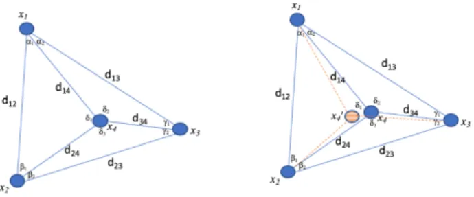
Fig. 1. Sensor geometric relationship.
to reduce their dilation before they are injected in a method, such as mMDS, where all segment contributions are treated equally.
III. GEOMETRICEDM RESOLUTION FORFTM A. Wall Remover - Minimization of Asymmetric Errors
One first contribution of this paper is a method to reduce dilation asymmetry. Space dimension is resolved using other techniques (e.g. RSSI-based). A strong obstacle between two stations, say x3 and x4, can cause their distance to appear
stretched. This stretch may not appear between x3 or x4
and other stations (e.g. x3x2 or x4x2). A good resolution
is therefore ‘not’ to average the error, but locate it, then attenuate it locally if possible. Geometry provides great tools to this mean, that can reduce the distance error only when it is directional, thus outputting a matrix ˜D which k factor is closer to uniformity. It should be noted that the purpose of such method should not be to fully solve the MDS problem, as some pair distances are usually not known, and the method has a limited scope .
In many cases, we can select 4 stations such that one of them is within the triangle formed by the three others, as represented in the left part of Figure 1. The triangle is scalene, but the same principle applies to any triangle. A fourth sensor x4 is found
within the (x1, x2, x3) triangle. Sides can be expressed from
other sides and angles. For example, d24 can be expressed
as d224 = d212 + d214− 2d12d14cos(α1). We could also use
a similar equation to express α1. Thus, angles and missing
distances can be found from known distances. However, in a noisy measurement scenario, inconsistencies are found.
For example, an evaluation of the triangle (x1, x2, x4)
may be consistent with the left side of Figure 1, but an evaluation of triangle (x1, x3, x4) may position x4 in the
hashed representation x04 of the right part of Figure 1. The most probable reason for the inconsistency is noise, an obstacle or a reflection source between x3 and x4. Other possibilities
can be found, for example a larger dilation for d12 than for
d24 and d14. But as more comparisons are performed, the
inconsistency re-appears when the pair is tested against other points, thus making the obstacle a likely cause. Thus, we propose a method where a learning machine, that we call a geometric wall remover engine, is fed with all possible distances in the matrix and compares all possible iterations of
sensors forming a triangle and also containing another stations. Each time a scenario matching the right side of Figure 1 is found, the algorithm learns the asymmetry and increases the weight w of the probability p that the matching segment (x3x4
in this example) has an overly stretched kij factor.
At the end of the first training iteration, the system outputs a sorted list of segments with the largest stretch probabilities, then attempts to reduce the largest stretch by applying to the affected segment distance a contraction factor ζij (this
can be a step increment, similar to other machine learning algorithms learning rate logic, or be proportional to the stretch probability). The system then runs subsequent iterations on the same principles, until the stretch of each segment falls within acceptable range of the others.
This method has the merit of surfacing points internal to the constellation that display large k factors, but is also limited in scope and intent. In particular, it cannot determine large k factors for outer segments, as the matching points cannot be inserted within triangles formed by other points. However, its purpose is to limit the effect of asymmetries, not to solve the entire matrix.
B. Iterative algebro-geometric EDM Resolution
The Wall Remover method can be used on its own to reduce asymmetry before using classical EDM techniques. It can also be used in combination with the iterative method proposed in this section, although the iterative method has the advantage of also surfacing dilation asymmetries, and thus could be used directly (without prior dilation reduction). Combined together, these two techniques provide better result than standard EDM techniques.
EDM resolution addresses two contiguous but discrete prob-lems: matrix completion and matrix resolution. In most cases, the measured distance matrix ˜D has missing entries (stations out of range of each other) and a first task is to complete the matrix by estimating these missing distances. Once the matrix contains non-zero numerical values, the next task is to resolve inconsistencies and find the best possible distance combination.
Several methods solve both problems with the same algo-rithm. Dokmanic et al. [4] provide a description of the most popular implementations. We propose a geometric method, which first uses partial matrix resolution as a way to project station positions geometrically onto aR2 plane, then a mean
cluster error method to identify individual points in individual sets that display large asymmetric distortions (and should therefore be voted out from the matrix reconstruction). By iteratively attempting to determine and graph the position of all possible matrices for which point distances are available, then by discarding the poor (point pairs, matrices) performers and recomputing positions without them, then by finding the position of the resulting position clusters, the system reduces asymmetries and computes the most likely position for each station.
The details of each step, along with the mathematical proofs, can be found in the research report by the same
authors [8]. The principles are as follows. The measured distance matrix ˜D of n station distances is separated in all possible sub-matrices ˜Dm of size 2 ≤ m ≤ n. A pivot xi
is chosen iteratively in ˜Dm. For each iteration, xi is set as
the origin, and xi = (0, 0). The next point xj is iteratively
set along the x-axis, and xj = ( ˜dxixj, 0). If m > 2, then
the position (uxl, vxl) of each other point xl of the set
{xi, xj, xl} is found using standard triangular formulas and
where: uxl= xlx2j−xix2l−xix2j −2xixj and vxl= q xix2l − u2xl
The calculated (uxl, vxl) are always positive, but their
sign can be corrected where needed based on the distance comparison between points on the graph. Later iterations use other points (xi = (0, 0)) as reference, coordinate translation
then rotation is used to align the next graph to the previous one, using common points successively as the reference (to align the graphs and yet avoid centering all graphs on xi).
As measured distances are noisy, at the end of the iterative process, all points associated with a stations are not perfectly overlapping, but form a cluster, which center can be deter-mined by a simple coordinate mean calculation. Projections that are congruent will display points that are close to one another for a given cluster. The graph will also display some representations that display large asymmetric deviations, caused by a dilation factor k different for a station pair than for the others. The geometric Wall Remover method is intended to reduce such effect. As it acts on the angles of adjacent triangles, it is more precise than this section of our proposed method. However, it may happen that the dilation occurs among pairs than the geometric Wall Remover cannot identify (for example because the pair is formed with stations at the edge of the constellation) and this method complements it.
The deviation also surfaces matrices coherence. A coherent matrix contains a set of distances displaying a similar dilation factor k. An incoherent matrix contains one or more distance displaying a k factor largely above or below the others. For example, several stations may be separated from each other by walls, but be in LoS of a common station, which will display a k factor smaller than the others. Stations that display good coherence in multiple matrices are efficient anchors (while those positioned in a challenging location are poor anchors for any iteration).
An additional step is therefore to identify good, medium and poor anchors and discard distances that were computed using poor anchors. This is done by computing the Euclidean dis-tance between each point position from a given matrix to the cluster center for that point. Points that are far from the cluster center are deemed poor anchors. Matrices using this station as an anchor are removed from the batch and clusters are recomputed without these stations’ contribution as anchors. As the computation completes, each cluster center is used as the best estimate of the associated station position. By reducing the variance of the dilation factor k, by removing sub-matrices and station pairs that bring poor accuracy contribution, this
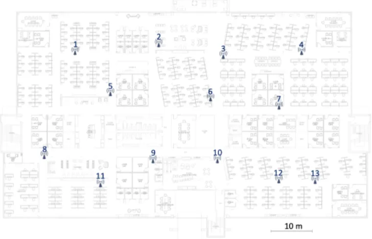
Fig. 2. Experimental setup.
method outperforms standard EDM completion methods when RN is known, because it incorporate asymmetries evaluation
and reduction as it computes the most likely anchor positions. IV. EXPERIMENTALVALIDATION
A. Experiment Methodology
We tested this method in a representative building that is a three-storey office building with cubicle areas alternating with blocks of small offices. Our testbed is installed on the second floor. The wall structure is irregular, causing different reflection and absorption patterns for each AP pair. The floor already has Wi-Fi coverage. One FTM device equipped with Intel 8260 cards is positioned near (one foot away) each of the 13 existing APs, near ceiling level, as represented in Figure 2. Ground truth distances are known from floor plan blueprint and onsite laser ranging. The FTM stations are configured to successively act as ISTAs and RSTAs. The system is left active for two days. Every hour, the system wakes up, each ISTA ranges against the detected RSTAs on various channels for 10 minutes and logs the result. At the end of the collection phase, the logs of all stations are collected and injected into the learning machine. Mobile stations are also walked around the building. GPS accuracy utilities are installed on different phones, that surface outside an error of less than half a meter on average. Inside the building, accuracy collapses.
Observing the distance matrices immediately makes appar-ent the challenges in mMDS. The ground truth 13∗13 distance matrix surfaces 9 positive eigenvalues, but only 2 of these are large, indicating a 2-dimensional geometrical object. The measured FTM matrix surfaces ‘only’ 7 positive eigenvalues, but all of them are large.
As such, it is clear that the distance matrix alone is not sufficient to assert the dimensionality of the space. However, complementing with RSSI evaluation easily solves the issue. Two APs (AP15 and AP16) are positioned on the upper floor above AP05 and AP06 respectively. A simple comparison of the observed signal and measured distance shows that AP15 signal to any AP on the lower floor systematically appears
Fig. 3. Measured distances to ground truth ratios, and pairs identified by the geometric wall remover method as ‘abnormal’.
12 to 28 dB below the pairwise signal between these APs at equivalent distance. By contrast, AP16 to AP15 signal appears 10 to 25 dB above the signal to any other AP at comparable distance. This result immediately indicates that AP15 and AP16 are on a different floor from the others (and that both AP15 and AP16 are on the same floor), allowing us to easily group APs on floors.
B. Geometric Wall Remover Phase
Some stations are positioned in open spaces, but others are placed in challenging locations, conference rooms or corridors, from where no clear LoS can be established to other stations. In some cases, the nLoS condition has no effect on the range mean (as all neighbors can only be reached through walls), but in some others, ‘canyon conditions’ appear, where strong reflections against walls cause the dilation factor to vary from with directionality.
Figure 3 displays the ratio between the mean of the mea-sured distance and the ground truth. The distances that the geometric wall remover engine identifies as deviating from the others are highlighted. Some stations are out of range from one another (e.g. station 1 against station 13) and are not addressed in this phase.
As can be observed, the geometric wall remover engine cor-rectly identifies most incorrect distances, except those affect-ing stations positioned at the edge of the floor. A contraction factor ζ is applied to the segment with worst stretch (the step value of ζ was chosen to be static and small, set to 0.98). As more iterations were run, each with a ζ factor applied to the worst offender, the number of reported abnormal distances decreases, until, on the last iteration, the engine does not surface any more anomaly. At this point, the largest deviation from the ground truth (for the flagged pairs) was brought down to 1.13. This validation indicates that the geometric wall remover can correctly identify inner outliers and reduce the associated error, without distorting the graph (over or under reduction).
C. Iterative algebro-geometric phase
In this phase, we start with the largest possible matrix. A matrix of size 13 is of course of low interest, as there is a single possible ranging outcome. Iteratively, the engine finds that a matrix of size 12 also offers a single solution, because the table contains several stations that are not of range of each other, thus causing some pairs to show NaN distance. A matrix of size 9 starts allowing for more than one pivot. As the matrix size decreases, more combinations appear and noise increases.
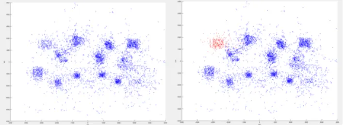
Fig. 4. Position graph of matrix size 5 (left), sensor 4 highlight in red (right).
Fig. 5. Clusters for sensors 2, 3, 5 and 6, before (left) and after (right) outlier suppression.
The process repeats iteratively. With smaller matrices and more combinations, clusters start to appear for each station, with various densities (mean distance from cluster center) as can be seen in Figure 4 (left). Each point to sensor identifier is known, and thus individual sensor clusters can be graphed as seen in Figure 4 (right), then treated separately if needed.
Clusters display different density. For each cumulative graph, cluster centers are computed and the mean cluster radius ri compared between clusters. Then, outliers (points
more than 2σ away from the cluster center) are removed from each cluster as displayed in Figure 5 (for better legibility, only 4 stations from the building are plotted).
After removing the outliers, each station cluster center is re-computed. The final cluster centers are displayed in Figure 6. Ground truth positions are green circles, the computed cluster position for each station is represented as a red star. The maximum error is observed at 1.1143 meter.
At this stage, the relative station positions are estimated, but their orientation is not known. However, using the ranging information from one or more mobile phones, walking outside the building, to two or more stations, and sending to the AP the GPS location of the mobile phone as seed, the graph can be rotated to its correct orientation and the phone GPS location can be used to populate the LCI values of all stations on the graph.
D. Comparison with other methods
Noisy EDM completion is a complex problem. Proposed solutions are many, and tend to be tailored to specific problem spaces. We will limit our comparison to the main methods listed in [4]. Naturally, using classic MDS boils down to performing an eigenvalue decomposition and geometric cen-tering. As the matrix is noisy, the error is large. Additionally, the algorithm interprets missing distances as 0 values, which
Fig. 6. Cluster center position computation (red star) vs ground truth position (green circles).
Fig. 7. Classical MDS projection with raw data (left) and after NaN distances resolution (right) in Building 1.
introduces irreconcilable inconsistencies in the matrix in all dimensions. The effect is worsened when the projection is constrained into R2, as can be seen in Figure 7 (left). This effect can be attenuated by constructing and overlapping partial matrices for which distances are known [1]. Even in this case, the effect of asymmetry is visible, resulting in a large error space (Figure 7, right).
Many optimizations methods aim at finding missing ele-ments from a matrix that is assumed to be noiseless. This assumption is necessary to maintain convexity, but with the consequence of being unusable in our scenario. For incomplete and noisy matrices, a classical solution is to use semi-definite relaxation. This technique has multiple variants to adapt to different matrix sizes or sparsity scenarios, and both [1] and [7] are typical illustrations of the associated reasoning. In all cases, the goal is to bound the rank of the Gram matrix to the target dimension space, thus constraining the number of positive and non-null eigenvalues. The process is efficient, especially for large matrices. As it proceeds iteratively, it also has the virtue of minimizing the error. However, the error is still affected by asymmetries and therefore sub-optimal for asymmetric scenarios like FTM.
V. CONCLUSION
We presented a method to solve noisy Euclidian distance matrices (EDM). We showed that in the case of station
time-of-flight measurements, measured distances are dilations of ground truth distance, but that the dilations are asymmetric, thus rendering classical EDM methods generally inaccurate, as they tend to assume noisy symmetry and therefore tend to center the error. We propose a machine learning method for identifying and reducing noise asymmetry based on evalua-tion of angles within overlapping triangles. We then propose a second machine learning method, aimed at graphing the positions of stations derived from distance sub-matrices, and at identifying and removing combinations that surface excessive distances, thus progressively removing edge asymmetries and reducing the distance errors. We show that this method outper-forms standard EDM resolution methods. In future works, we will examine how this method can be extended to 802.11az, where some stations can stay entirely passive, building their location from the observation of FTM exchanges between other stations.
REFERENCES
[1] E. Candes and Y. Plan. Matrix completion with noise. Proceedings of the IEEE, 98(6):925–936, Jun 2010.
[2] J. Dattorro. CONVEX OPTIMIZATION † EUCLIDEAN DISTANCE GEOMETRY 2e. December 2019.
[3] L. Doherty, K. S. J. Pister, and L. E. Ghaoui. Convex position estimation in wireless sensor networks. In Twentieth Annual Joint Conference of the IEEE Computer and Communications Society, pages 1655–1663, 2001. [4] I. Dokmanic, R. Parhizkar, J. Ranieri, and M. Vetterli. Euclidean distance matrices: Essential theory, algorithms, and applications. IEEE Signal Processing Magazine, 32(6):12–30, Nov. 2015 2015.
[5] N. Dvorecki, O. Bar-Shalom, L. Banin, and Y. Amizur. A machine learning approach for wi-fi rtt ranging. In Proceedings of the 2019 International Technical Meeting of The Institute of Navigation, pages 435–444, 01 2019.
[6] T. Eren and et. al. Rigidity, computation, and randomization in network localization. IEEE INFOCOM, 4:2673–2684, 2004.
[7] X. Guo, L. Chu, and X. Sun. Accurate localization of multiple sources using semidefinite programming based on incomplete range matrix. IEEE Sensors Journal, 16(13):5319–5324, July 2016.
[8] J. Henry, I. Hrasko, Y. Busnel, R. Ludinard, and N. Montavont. A Geometric Approach to Noisy EDM Resolution in FTM Measurements. https://www.dropbox.com/s/gk2600vtky7d4c0/Geometric approach to
noisy EDM resolution in FTM measurements-11.pdf?dl=0, 2020. [Online; accessed 13-June-2020].
[9] D. Jacobs. Multidimensional scaling: More complete proof and some insights not mentioned in class. 2016.
[10] M. Kjaergaard and et al. Indoor Positioning Using GPS Revisited, pages 38–56. 2010.
[11] L. Liberti. Distance geometry and data science, 2019.
[12] R. Liu, C. Yuen, T. Do, and U. Tan. Fusing similarity-based sequence and dead reckoning for indoor positioning without training. IEEE Sensors Journal, 17(13):4197–4207, 2017.
[13] X. Liu, S. K. Nath, and R. Govindan. Gnome: A practical approach to nlos mitigation for gps positioning in smartphones. pages 163–177, 01 2018.
[14] L. Pan, C. Cai, R. Santerre, and X. Zhang. Performance evaluation of single-frequency point positioning with gps, glonass, beidou and galileo. Survey Review, 49(354):197–205, 2017.
[15] Y. Polk, M. Linser, M.Thomson, and B. Aboba. Dynamic Host Config-uration Protocol Options for Coordinate-Based Location ConfigConfig-uration Information. RFC 6225, RFC Editor, July 2011.
[16] J. Tsang and R. Pereira. Taking all positive eigenvectors is suboptimal in classical multidimensional scaling. ArXiv, abs/1402.2703, 2016. [17] A. Yassin, Y. Nasser, M. Awad, A. Al-Dubai, R. Liu, C. Yuen,
R. Raulefs, and E. Aboutanios. Recent advances in indoor localization: A survey on theoretical approaches and applications. IEEE Communi-cations Surveys Tutorials, 19(2):1327–1346, 2017.