HAL Id: hal-01610408
https://hal.sorbonne-universite.fr/hal-01610408
Submitted on 4 Oct 2017
HAL is a multi-disciplinary open access
archive for the deposit and dissemination of
sci-entific research documents, whether they are
pub-lished or not. The documents may come from
teaching and research institutions in France or
abroad, or from public or private research centers.
L’archive ouverte pluridisciplinaire HAL, est
destinée au dépôt et à la diffusion de documents
scientifiques de niveau recherche, publiés ou non,
émanant des établissements d’enseignement et de
recherche français ou étrangers, des laboratoires
publics ou privés.
Distributed under a Creative Commons Attribution| 4.0 International License
Sea Surface Temperature of the mid-Piacenzian Ocean:
A Data-Model Comparison
Harry Dowsett, Kevin Foley, Danielle Stoll, Mark Chandler, Linda Sohl, Mats
Bentsen, Bette Otto-Bliesner, Fran Bragg, Wing-Le Chan, Camille Contoux,
et al.
To cite this version:
Harry Dowsett, Kevin Foley, Danielle Stoll, Mark Chandler, Linda Sohl, et al.. Sea Surface
Tempera-ture of the mid-Piacenzian Ocean: A Data-Model Comparison. Scientific Reports, NaTempera-ture Publishing
Group, 2013, 3 (1), pp.2013. �10.1038/srep02013�. �hal-01610408�
Sea Surface Temperature of the
mid-Piacenzian Ocean: A Data-Model
Comparison
Harry J. Dowsett
1, Kevin M. Foley
1, Danielle K. Stoll
1, Mark A. Chandler
2, Linda E. Sohl
2, Mats Bentsen
3,
Bette L. Otto-Bliesner
4, Fran J. Bragg
5, Wing-Le Chan
6, Camille Contoux
7,8, Aisling M. Dolan
9,
Alan M. Haywood
9, Jeff A. Jonas
2, Anne Jost
8, Youichi Kamae
10, Gerrit Lohmann
11, Daniel J. Lunt
5,
Kerim H. Nisancioglu
3, Ayako Abe-Ouchi
6,12, Gilles Ramstein
7, Christina R. Riesselman
1,
Marci M. Robinson
1, Nan A. Rosenbloom
4, Ulrich Salzmann
13, Christian Stepanek
11,
Stephanie L. Strother
1,13, Hiroaki Ueda
10, Qing Yan
14& Zhongshi Zhang
14,31United States Geological Survey, Reston, Virginia, 20192, USA,2Columbia University - NASA/GISS, New York, NY, 10025,
USA,3Bjerknes Centre for Climate Research, Bergen, Norway,4National Center for Atmospheric Research, Boulder, Colorado,
80305, USA,5School of Geographical Sciences, University of Bristol, Bristol BS8 1SS, UK,6Atmosphere and Ocean Research
Institute, University of Tokyo, Kashiwa 277-8564, Japan,7Laboratoire des Sciences du Climat et de l’Environnement/IPSL, UMR
CEA-CNRS-UVSQ, Orme des Merisiers, 91191 Gif-sur-Yvette, France,8UPMC Universite´ Paris 06 & CNRS, Sisyphe, 75005
France,9School of Earth and Environment, University of Leeds, Leeds, UK,10Graduate School of Life and Environmental Sciences,
University of Tsukuba, Tsukuba, Japan,11Alfred Wegener Institute for Polar and Marine Research, Bremerhaven, Germany, 12Research Institute for Global Change, Japan Agency for Marine-Earth Science and Technology, Yokohama, Japan,13Department
of Geography, Faculty of Engineering and Environment, Northumbria University, Newcastle upon Tyne, NE1 8ST, UK,14Institute of
Atmospheric Physics, Chinese Academy of Sciences, Beijing, China.
The mid-Piacenzian climate represents the most geologically recent interval of long-term average warmth
relative to the last million years, and shares similarities with the climate projected for the end of the 21
stcentury. As such, it represents a natural experiment from which we can gain insight into potential climate
change impacts, enabling more informed policy decisions for mitigation and adaptation. Here, we present
the first systematic comparison of Pliocene sea surface temperature (SST) between an ensemble of eight
climate model simulations produced as part of PlioMIP (Pliocene Model Intercomparison Project)
with the PRISM (Pliocene Research, Interpretation and Synoptic Mapping) Project mean annual SST
field. Our results highlight key regional and dynamic situations where there is discord between the
palaeoenvironmental reconstruction and the climate model simulations. These differences have led to
improved strategies for both experimental design and temporal refinement of the palaeoenvironmental
reconstruction.
T
he deep-time geological record contains responses of the climate system to a wide range of internal and
external forcings as well as documentation of intricate short- and long-term feedbacks. While modeling
studies of more recent past climate intervals, like the Last Millennium (LM) and the Last Glacial Maximum
(LGM), provide useful information about the future of our climate system and are being incorporated into the
next Intergovernmental Panel on Climate Change (IPCC) assessment, palaeoclimate modeling of more ancient
time periods have been unable to reproduce some of the key large-scale features associated with periods of
extreme global warmth, and it is important that we gain a better understanding of such discrepancies.
Deep-time climates afford us an opportunity to explore climate sensitivity to a range of atmospheric CO
2levels, to
understand how heat is transported during warm climate intervals, to gain insight into the controls on
pole-to-equator thermal gradients, and to evaluate the stability of ice sheets and the response of sea level during warmer
climates. Anthropogenic changes could affect Earth’s climate for hundreds to thousands of years, thus analysis
and understanding of the most recent deep-time interval of warmth – similar in magnitude to that projected for
the end of the 21
stcentury – is relevant to our understanding of future climate and discussion of adaptation and
mitigation policies.
SUBJECT AREAS:
CLIMATE AND EARTH SYSTEM MODELLING MARINE BIOLOGY PALAEOCEANOGRAPHY PALAEOCLIMATE
Received
25 January 2013
Accepted
31 May 2013
Published
18 June 2013
Correspondence and requests for materials should be addressed to H.J.D. (hdowsett@ usgs.gov)The Pliocene Epoch (5.332 Ma to 2.588 Ma) spans an interval of
global warmth with high-frequency, low-amplitude variability
tran-sitioning to high-frequency, high-amplitude variability associated
with the initiation of Northern Hemisphere glaciation. The U.S.
Geological Survey’s Pliocene Research, Interpretation and Synoptic
Mapping (PRISM) group selected for study the most recent interval
within the Pliocene (3.264 to 3.025 Ma) known to have temperatures
above preindustrial (PI) levels. This interval within the Pliocene, the
middle part of the Piacenzian Age, is particularly attractive for
palaeoclimate studies because many of the first-order boundary
con-ditions were little different than today: continents and ocean basins
were near their present geographic positions and the flora and fauna
of the Late Pliocene was in large part identical to present day,
allow-ing for modern analog-type reconstructions of the
palaeoenviron-ment
1. Chronology for Piacenzian sequences within deep-sea cores
can usually be well-resolved from many magnetobiochronologic
events, coupled with an ever-increasing number of orbitally-tuned
chronologies
2.
The ‘‘PRISM interval’’ has been the focus of two decades of
intens-ive investigations into all aspects of the climate system, resulting in a
series of palaeoenvironmental reconstructions: PRISM0, PRISM1,
PRISM2 and the current PRISM3
3–30. PRISM data have been used
in a number of climate modeling studies to explore conditions
dur-ing this last great interval of global warmth
31–39. A natural evolution
of these individual modeling studies was the formation of an
orga-nized model intercomparison project for the Pliocene, which
includes many of the leading climate models that contribute IPCC
simulations.
The Pliocene Model Intercomparison Project (PlioMIP) is a
sub-component of the Palaeoclimate Modelling Intercomparison Project
(PMIP
40,41;). The initial phase of PlioMIP includes two experiments,
both of which focus on the mid-Piacenzian time period equivalent to
the PRISM data sets: the first PlioMIP experiment employs
atmo-sphere-only general circulation models, and the second utilizes
coupled ocean-atmosphere models (see
42–54). Both experiments make
use of the PRISM3 versions of the boundary condition data sets
30.
In this paper we compare initial results of the second PlioMIP
experiment using mean annual sea surface temperature (SST) fields
derived from eight simulations (Figure 1), with PRISM mean annual
SST estimates at each of 100 locations in the PRISM3 marine
recon-struction (Figure 2). This comparison is used to document large-scale
features of the mid-Piacenzian surface ocean, assess where models
and data are in good general agreement and where they are not, and
also looks at the variability of the multi-model ensemble versus the
variability in the palaeodata-based estimates.
Results
Comparison of individual model and data anomalies (D
MODELand
D
PRISM, respectively, see ‘‘Methods’’) on a site-by-site basis identifies
a greater range of warming in the reconstructed SST (,10uC spread
in D
PRISM). The models are the most inconsistent with each other,
and with the PRISM data in the North Atlantic region (Figure 3).
This area is, of course, complex given that a myriad of strong
feed-backs can affect the region, including changes in sea ice, the Gulf
Stream current, Atlantic meridional overturning, and even the storm
tracks. Similar inconsistency in this region was shown among
the general circulation models (GCM’s) used in the IPCC 4
thassessment
55.
Individual models rarely show negative (i.e. Pliocene SST cooler
than present day) anomalies. Relative to the data, the
multi-model-mean anomaly (D
MMM) always shows small positive values and
exceeds 13uC at only two locations corresponding to core Site 722
on the Arabian Margin and Site 907 in the subarctic North Atlantic
(Figure 3).
Negative D
PRISMvalues are confined to the tropics and the
sub-tropical North Atlantic (Figures 2, 3). In the latter (area b in Figure 3),
these anomalies are isolated to land sections (outcrops) associated
with the western boundary current and others in the Mediterranean
Sea region. The subtropical estimates are from a combination of
planktonic foraminifer, ostracod and Mg/Ca palaeothermometers
and represent medium- to high-confidence sites (Figure 2). The
tropical sites showing negative D
PRISMvalues (area a in Figure 3)
are located near the equator in all ocean basins and are presently
associated with equatorial divergence. Small changes in position of
equatorial currents and upwelling cells along coastal regions could
explain apparent cooling at these locations.
Other upwelling sites from the Pacific (677, 847, 852, 1236, 1237,
1239), Atlantic (659, 661) and Indian Oceans (722) have some of the
largest D
PRISMvalues in the low-latitude data set based upon a
com-bination of planktic foraminiferal and alkenone palaeothermometry
and show basic agreement between proxies and between D
PRISMand
multi-model-mean anomalies (D
MMM) (Figure 3
30; Supplementary
information). Tropical sites in the PRISM3 data set collectively
indi-cate a mean anomaly of 11.08uC. The aforementioned sites have a
mean anomaly of 13.21uC. Removal of these sites greatly reduces the
magnitude of the mean tropical D
PRISM(to 10.4uC) and supports the
Dowsett et al.
28finding that low latitude SSTs, away from upwelling
centers, were indistinguishable from modern conditions.
Documenting the tropical sea surface temperature stability in the
Pliocene, particularly given evidence of substantial warming at high
latitudes, is of considerable importance for the appraisal of the
prim-ary climate drivers for this period. The multi-model ensemble from
the IPCC 4
thassessment report shows that greenhouse gas forcing of
less than a double-CO
2equivalent still yields a tropical warming of
Figure 1
|
Model sea surface temperature anomaly (DSST), calculated bysubtracting preindustrial from Pliocene sea surface temperature, as simulated by each of the eight PlioMIP models. (a) CCSM4, (b) COSMOS, (c) GISS-E2-R, (d) HadCM3, (e) IPSL CM5A, (f) MIROC4m, (g) MRI-CGCM2.3, (h) NorESM. Maps created using Panoply v.3.1.3 written by Robert B. Schmunk.
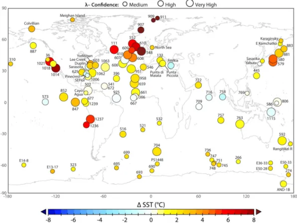
Figure 2
|
Map showing distribution of PRISM localities, sea surface temperature anomalies (DSST), calculated by subtracting modern from Pliocene sea surface temperature, and the l-confidence placed upon each locality estimate (relative size of circle, where larger circles represent greater confidence). Map created in iMap v.3.5 using World Vector Shoreline (NOAA National Geophysical Data Center, Date Retrieved 4/17/2011, http://www.ngdc.noaa.gov/mgg/shorelines/shorelines.html).Figure 3
|
Scatter plot of multi-model-mean anomalies (squares) and PRISM3 data anomalies (large blue circles) by latitude. Vertical bars on dataanomalies represent the variability of warm climate phase within the time-slab at each locality. Small colored circles represent individual model anomalies and show the spread of model estimates about the multi-model-mean. While not directly comparable in terms of the development of the means nor the meaning of variability, this plot provides a first order comparison of the anomalies. Encircled areas are (a) PRISM low latitude sites outside of upwelling areas; (b) North Atlantic coastal sequences and Mediterranean sites; (c) large anomaly PRISM sites from the northern hemisphere. Numbers identify Ocean Drilling Program sites discussed in the text.
more than 1uC by the middle of this century
55while recent Pliocene
simulations using the Goddard Institute for Space Studies (GISS)
ModelE2-R, a Coupled Model Intercomparison Project Phase 5
(CMIP5 ) model, found that Pliocene tropical warming exceeded
1uC with as little as 405 ppm CO
253. Although the existence of a
tropical thermostat mechanism cannot be entirely ruled out given
uncertainties in modeled cloud responses, most of the IPCC GCM’s
would support the lower-end estimates for Pliocene atmospheric
CO
2. The only locations in the tropics where the PRISM3 data do
indicate some warming tend to be in areas of present-day upwelling,
so most simulations, which show consistent warming at all
long-itudes, are still too warm compared with proxies.
A second region of offset between the D
MMMand D
PRISMexists in
the mid- to high northern latitudes. The majority of sites in Figure 3
(area c) are from the North Atlantic. The extensive warming at high
latitudes in the North Atlantic has been repeatedly
documen-ted
9,27,28,45and is also seen in terrestrial archives of surface air
tem-perature (e.g.
56,57). Mid-latitude sites (410, 548, 552, 606, 607, 608 and
610) are the very highest confidence sites in the PRISM3 data set, and
the large inter-model spread in this region may be due to the highly
variable position of the Gulf Stream—North Atlantic Drift and the
resolution of the different models
45. However, the magnitude of the
warming in the mid- to high-latitude North Atlantic, in both D
MMMand any D
MODEL, is small compared to D
PRISM. While the variability
of D
PRISM(a function of the within-time-slab variability at those
localities) and the spread of the individual D
MODELresults about
the D
MMMoverlap in many cases (Figure 3), there is no way to
directly compare these uncertainty measures, and there exists a
con-sistent offset between data and models.
Four sites in Figure 3 (area c) are outside the North Atlantic. Sites
579 and 580 are located in the North Pacific Kuroshio Extension.
Analysis of the diatom assemblages at both sites suggests moderate
warming over present day conditions within the PRISM interval
8,13.
Some but not all PlioMIP simulations pick up this North Pacific
warming (relative to PI conditions) (Figure 1). New faunal data from
ODP Site 1208, located beneath the Kuroshio Extension, show little
change in mean annual temperature relative to present day but
sug-gest greatly reduced seasonality (5uC), with winter temperatures
warmer during the Pliocene (Supplementary material). This is
essen-tially the same pattern exhibited by the Gulf Stream in the North
Atlantic. This reduced seasonality is not demonstrated by PlioMIP
simulations.
Sites 1014 and 1021, from the upwelling cell off the west coast of
North America, show Pliocene warming (relative to today)
docu-mented by both faunal and alkenone palaeothermometry of 6uC–
8uC, which is not simulated by any of the models (area c of Figure 3).
Reed-Sterrett et al.
58suggest the cause may be due to a shoaling
thermocline, but an analysis of seasonal vertical temperature profiles
from the MIROC4m and GISS-E2-R simulations show no change to
the thermocline between Pliocene and PI (preindustrial).
Sites 1236 and 1237 are both situated on the Nazca Ridge. Site 1236
is located just seaward of the main path of the cool, northward
flowing Peru-Chile Current while Site 1237 is located near the
east-ern edge of the current and associated upwelling. Proxy SST data
show warmer upwelling conditions during the Pliocene than exist
today in the region, analogous to the upwelling region off the Pacific
coast of North America (Figure 2). The D
MMMvalues do not capture
this, but some PlioMIP simulations (GISS-E2-R and HadCM3) do
show warmer regional anomalies (Figure 1) and the MIROC4m
simulation shows a deepening of the mixed layer during the
Pliocene relative to the PI.
Large scale features.
Several large-scale first-order features of the
Pliocene climate can be found in both data reconstructions and
model simulations. Models are generally in good agreement with
estimates of Pliocene SST in most regions except the North
Atlantic and upwelling regions in the tropics and subtropics
(Figures 1, 2). Despite the complications of variability within the
PRISM time slab and the spread shown by the different PlioMIP
simulations, there is a fundamental divergence between the two
data sets that increases with increasing latitude. This decoupling
may stem from a number of sources, including the resolution of
the models, differing model parameterizations of subgrid-scale
features such as clouds, the highly variable nature of the
mid-latitude North Atlantic, or the nature of the Gulf Stream – North
Atlantic Drift Current
45.
Polar amplification of SSTs is one of the principal signatures of the
PRISM data set, with a maximum temperature increase observed in
the North Atlantic. However, no such extreme is evident in the
MMM data (Figure 3). While individual models show various levels
of polar amplification, none are equivalent in magnitude to the
PRISM data. Conversely, low-latitude warming is common to all of
the PlioMIP simulations, but is not observed in the PRISM data away
from upwelling cells. Suggestions that increased oceanic and/or
atmospheric heat transport during the Pliocene helped flatten the
meridional temperature gradient are not unequivocally supported by
the MMM data, because individual model simulations show a wide
range of heat transport response
59.
Although general ocean surface circulation, based upon global
distribution of SSTs, appears to have been broadly similar between
the Pliocene and today, patterns of warming seen in the PRISM data
in both the North Atlantic and North Pacific could indicate that
western boundary currents were more vigorous or that meridional
overturning was enhanced. Unfortunately, climate models do not
have a consistent Pliocene response with regards to either meridional
overturning or ocean heat transport
59.
Reduced seasonality, a phenomenon more characteristic of the
tropics in the modern, can be documented farther north during
the Pliocene based upon analysis of palaeontological assemblages
found in coastal regions (e.g. Ref. 60–62).
In the Southern Ocean, poleward displacement of palaeo-fronts is
documented in the PRISM data by changes in sedimentology,
paleontology and productivity
14,16that demonstrate the Pliocene
Antarctic Polar Front was as much as 6u latitude further south than
today. The corresponding adjustments of isotherms are in close
agreement with the PlioMIP simulations, especially when the
vari-ability of both is taken into account (Figure 3).
Discussion
Features determined by the analysis of palaeontological and
geo-chemical data as well as output of the PlioMIP simulations document
the overall warming of surface waters of the Pliocene ocean.
Large-scale circulation (i.e., the existence of but not necessarily
position of subtropical gyres) appears to have been similar in both
data reconstructions and model simulations, but the differences in
resolution between models and the variability introduced by the
PRISM time slab averaging procedures tend to obscure important
details. The PlioMIP simulations of mean annual temperature
(MAT) do not pick up the magnitude of warming in upwelling
regions documented by geochemical and palaeontological proxies
in the PRISM data. An initial analysis of seasonal vertical
temper-ature profiles from seven of the eight PlioMIP simulations in the Peru
Upwelling region shows a simple temperature offset between PI and
Pliocene, but no change to thermocline depth. Only one model,
MIROC4m, shows a clearly deeper thermocline and concomitant
mixed layer during the Pliocene. Tropical cyclones may play an
important role in vertical mixing of the upper ocean
63,64, but
dem-onstrating that to be the case for the PlioMIP simulations will require
analysis beyond the scope of the current study.
The overall D
MMMfield is in agreement with D
PRISMvalues in most
regions; however, models do not achieve the level of high-latitude
warming seen in the North Atlantic and Arctic data. Reduced sea ice
Table
1
|Details
of
coupled
atmosphere-ocean
climate
models,
boundary
conditions,
published
climate
sensitivity
and
ocean
heat
transport
values
59from
PlioMIP
Experiment
2
Mode lI D Sponsor(s )Count ry Atmos phere Top Resolut ion Ocean Resolut ion Z Coord ., Top BC Se a Ice Dynam ics, Leads , Coupling Flu x adjustm ents, Land Soils, Plant s, Routing , PlioMIP Exp 2 Boundary Con ditions : Prefer red/Alternate Int egration Length (Years) Cl imate Sensitivit y (u C) Ocea n Heat Tran sport PL-PI (%) CCSM4 * Nationa lCenter for Atmosp heric Research, USA Top 5 2.2 hPa 0.9 u 3 1.2 5 u, L2 6 0.2 7 u–0. 64 u 3 1.1 25 u, L60 Depth, free surface Rhe ology, leads, melt ponds No adjustment s Layers, cano py, rou ting Alter nate 500 3.2 2 4 MIRO C4m Center for Climate Sys tem Research (Uni . Tokyo, N ational Ins t. for Env . Studies, Fro ntier Research Ce nter for Global Cha nge, JA MSTE C), JAPAN Top 5 30 km T42 (, 2.8 u 3 2.8 u) L20 0.5 u–1.4 u 3 1.4 u, L43 Sigma /depth free surface Rhe ology, leads No adjustment s Layers, cano py, rou ting Preferr ed 1400 4.0 5 2 7 HadC M3 Hadle y Cent re for Cl imate Pr ediction and Rese arch/M et O ffice U NITED KI NGDOM Top 5 5 hPa 2.5 u 3 3.7 5 u, L1 9 1.2 5 u 3 1.2 5 u, L20 Depth, rig id lid Free dri ft, lea ds No adjustment s Layers, cano py, rou ting Alter nate 500 3.1 2 7 GIS S-E2-R * NASA/GIS S, USA Top 5 0.1 hPa 2 u 3 2.5 u,L 4 0 1 u 3 1.25 u, L32 Mass/ are a, free surface Rhe ology, leads No adjustment s Layers, cano py, rou ting Preferr ed 950 2.7 4 COS MOS Alfred We gner Ins titute GER MANY Top 5 10 hPa T3 1 (, 3.75 u 3 3.7 5) u, L19 bi polar orthogo nal curvil inear GR30 , L40 (formal 3.0 u 3 1.8 u) D epth, free surface Rhe ology, leads No adjustment s Layers, cano py, rou ting Preferr ed (for details see Stepa nek and Lohmann (20 12)) 1000 4.1 6 IPSL CMS A * Laboratoire des Sci ences du Climat et de l’En vironne-ment FR ANCE Top 5 70 km 3.7 5 u 3 1.9 u, L3 9 0.5 u–2 u 3 2 u, L31 Free surface , Z-co ordinates Th ermo- dynamics , -Rhe ology, Lea ds No adjustment s Layers, cano py, rou ting, pheno logy Alter nate 750 3.4 2 MR I-CGCM 2.3 Meteoro logical Research Institute and Uni versity of Tsu kuba JA PAN Top 5 0.4 hPa T42 (, 2.8 u 3 2.8 u) L30 0.5 u–2.0 u 3 2.5 u, L23 Depth, rig id lid Free dri ft, lea ds Heat, fresh water and mome ntum (12 uS–12 uN) Layers, cano py, rou ting Alter nate 500 Eq uilibrium CS : 3.2 (Effe ctive CS : 2.9) 3 NorE SM Bjerknes Centr e for Cl imate Rese arch N ORWAY Top 5 3.5 hPa, T31, L2 6, (C AM4) G37 (, 3 u 3 3 u), L30 isopycnal lay ers and L2 nonisop ycnal lay ers sa me as CC SM4 No adjustment s same as CC SM4 Alter nate 1500 3.1 2 14 *denotes models used for IPCC 5th A ssessment Report.cover no doubt played a significant role in the high latitude warming
of the Pliocene. Continued refinement of the model
parameteriza-tions and proxy data for Arctic sea ice may improve the agreement
between PlioMIP simulations and warmth suggested by marine and
terrestrial data.
The mid-latitude North Atlantic is highly variable today, and this
is reflected in the high variance associated with the D
MMMin this
region. Future experiments aimed at understanding additional
for-cings and incorporating seasonal rather than mean annual SST may
help elucidate the spread in D
MMMin the mid latitude North Atlantic
region.
These PlioMIP simulations, performed with carefully controlled
boundary conditions and protocols, point to the need for a more
temporally refined data reconstruction with as broad geospatial
cov-erage as possible. The next phase of PlioMIP simulations will be
accomplished using a realistic near-modern orbital configuration
relevant to future climate discussions
65. If the oceanographic record
responds strongly to certain orbital periods in certain regions, the
time-slab methodology could produce a systematic bias in those
regions. Similarly, the time-slab may integrate different seasonality
in each measurement within the time-slab. In an attempt to reduce
uncertainty, the PRISM4 palaeoenvironmental reconstruction will
be correlated to marine isotope stage KM5c representing an
order-of-magnitude increase in chronologic resolution
66.
The PlioMIP model ensemble comparison to the PRISM3
palaeo-environmental reconstruction of SST represents the first systematic
data-model comparison for the mid-Piacenzian warm period. The
differences we identify between proxy data and models, if real,
pre-sents a significant challenge in assessing climate sensitivity beyond
the current period. Since the Pliocene is an optimal test-bed for
models, and in the face of current and future warming, it is
imper-ative that the disagreement in amplitude of warming be explored in
more detail with a focus on reducing uncertainty in climate proxies as
well as uncertainties in the models and their forcings.
Methods
PRISM Reconstruction.The PRISM mean annual temperature verification data set has 100 localities ranging from 77.9u South latitude to 80.4u North latitude and situated in every major ocean basin (Figure 2). Approximately 1/3 of the localities are confined to the Tropics and 1/3 are in the North Atlantic Basin. Twenty percent of the PRISM sites are located in the Southern Ocean. These data are derived primarily from quantitative faunal or floral analyses, augmented where possible with Mg/Ca and alkenone estimates45. The PRISM data have been examined in numerous articles
including1,18,30,39,45.
PRISM mean annual SST estimates represent a warm-peak-average, which is defined as the warm phase of climate from the interval between 3.264 Ma and
3.025 Ma at each locality. The use of a time-slab equivalent to ,240 Ky duration introduces variability about the estimated warm phase of SST, expressed as the standard deviation of the warm peak estimates within the time slab at each locality (See Supplementary Information Table S1).
Data have been assessed using the l-confidence scheme45. This provides a
measure of confidence based upon chronology, sample density, sample quality and type as well as performance of quantitative method used. l for included localities ranges from Very High to High to Medium and the percentage of sites
corresponding to each level are 29%, 34% and 36% respectively. Figure 2 shows the spatial distribution and confidence of the 100 PRISM localities (see also
Supplementary Table S1).
Models.The model simulations included in this paper are from CCSM4 (National Center for Atmospheric Research54), GISS-E2-R (NASA Goddard Institute for Space
Studies53), HadCM3 (Hadley Centre for Climate Prediction and Research52),
MIROC4m (Center for Climate System Research, National Institute for Environmental Studies, Frontier Research Center for Global Change44), COSMOS
(Alfred Wegner Institute48), IPSL CM5A (Laboratoire des Sciences du Climat et de
l’Environnement51), MRI-CGCM2.3 (Meteorological Research Institute and
University of Tsukuba50) and NorESM (Bjerknes Centre for Climate Research49).
Details of the models are found in Table 1 and in the corresponding publications. The GISS-E2-R, CCSM4 and IPSL CM5A models are the same versions used in IPCC 5th
assessment future climate simulations. Coupled ocean-atmosphere model simulations for the PlioMIP experiment will be available from the PMIP3 project https://pmip3.lsce.ipsl.fr/.
In an attempt to standardize the PlioMIP simulations, all models were initialized and run using an identical (to the extent possible) experimental design and protocol (Table 2; see also43). Of the eight models, three (MIROC4m, COSMOS and
GISS-E2-R) used the preferred Pliocene boundary conditions, meaning each model’s land/sea mask was altered to reflect a 25-meter increase in Pliocene sea level, the existence of ocean in place of the West Antarctic Ice Sheet, and the removal of Hudson Bay (which is a result of Pleistocene ice sheet geography).
For each model in the PlioMIP ensemble, the Pliocene simulations were run until the individual modeling groups determined that their models had achieved an equilibrium state; integration times varied from 500 to 1500 years (Table 1). Twelve monthly SST fields were then averaged over the last 30 years of the run to develop a mean annual SST data set. Figure 1 shows the change in SST, Pliocene minus PI, simulated by each of the eight PlioMIP models. In this study, data points representing the PRISM localities are selected directly from the contributed datasets to avoid biases due to interpolation during re-gridding.
Comparison of anomalies.Analysis of the global and regional performance of the eight PlioMIP models is based upon comparison to the multiple proxy SST anomalies documented in45, which are referenced to the mid-20th century calibration of
Reynolds and Smith67. We focus on comparing data and model SST anomalies rather
than absolutes to avoid biases introduced by the effect of latitude on absolute SST (warmer at lower latitudes and cooler at higher latitudes). Testing the commonality between the anomalies produced by the model and data affords a more accurate test of the model response to Pliocene boundary conditions34,39.
Part of model–data disagreement is related to differences in the control (PI) simulation for each model. We corrected each model anomaly by subtracting a term equivalent to the difference between the mid 20thcentury calibration used by the
palaeontological data and PI conditions39:
Table 2 | Forcings and boundary conditions for PlioMIP Experiment 2 Pliocene and preindustrial simulations
Experiment 2 Protocol Preferred Alternate Control
Greenhouse gases
CO2(ppm) 405 405 280
N2O (ppb) As PI control As PI control 270
CH4(ppb) As PI control As PI control 760
CFCSs As PI control As PI control 0
O3 As PI control As PI control Local Modern
Orbital
Eccentricity 0.016724 As PI control 0.016724
Obliquity (u) 23.446u As PI control 23.446u
Perihelion (180u) 102.04u As PI control 102.04u
Boundary Conditions
Land/Sea Mask land_fraction_v1.1 local modern land/sea mask Local Modern
Topography topo_v1.1* topo_v1.4* Local Modern
Ice Sheets biome_veg_v1.3or biome_veg_v1.2or Local Modern
mbiome_veg_v1.3 mbiome_veg_v1.2
Vegetation biome_veg_v1.3or biome_veg_v1.2or Pre-industiral
mbiome_veg_v1.3 mbiome_veg_v1.2 including land use
DPRISM~PRISMPLIO{RSMODERN
DMODEL~MODELPLIO{RSMODERN{
MODELPREINDUSTRIAL{HadISSTPREINDUSTRIAL
ð Þ
where PRISMPLIOis the PRISM3 mean annual SST estimate at each locality (45,68, this
paper); RSMODERNis the modern observed temperature at each PRISM locality
determined from61; MODEL
PLIOis the mean annual SST value sampled at each
PRISM locality from the model SST field as described above; MODELPREINDUSTRIAL
is the mean annual SST value sampled at each PRISM locality from the model control simulation; HadISSTPREINDUSTRIALis the mean annual SST sampled at each PRISM
locality from a PI data set which is a hybrid of observational and modeled data69.
1. Dowsett, H. J. The PRISM palaeoclimate reconstruction and Pliocene sea-surface temperature. In Deep-time perspectives on climate change: marrying the signal from computer models and biological proxies (eds. Williams, M., Haywood, A. M., Gregory, J. & Schmidt, D. N), pp. 459–480 (Micropalaeontological Society Special Publication, Geological Society of London, 2007).
2. Wade, B. S., Pearson, P. N., Berggren, W. A. & Pa¨like, H. Review and revision of Cenozoic tropical planktonic foraminiferal biostratigraphy and calibration to the geomagnetic polarity and astronomical time scale. Earth Sci. Rev. 104, 111–142 (2011).
3. Dowsett, H. J. & Cronin, T. M. High eustatic sea level during the middle Pliocene: Evidence from the southeastern U.S. Atlantic Coastal Plain. Geology 18, 435–438 (1990).
4. Cronin, T. M. Pliocene shallow water paleoceanography of the North Atlantic Ocean based on marine ostracodes. Quat. Sci. Rev. 10, 175–188 (1991). 5. Dowsett, H. J. The development of a long-range foraminifer transfer function and
application to Late Pleistocene North Atlantic climatic extremes. Paleoceanography 6, 259–273 (1991).
6. Dowsett, H. J. & Poore, R. Z. Pliocene sea surface temperatures of the North Atlantic Ocean at 3.0 Ma. Quat. Sci. Rev. 10, 189–204 (1991).
7. Thompson, R. S. Pliocene environments and climates in the western United States. Quat. Sci. Rev. 10, 115–132 (1991).
8. Barron, J. A. Pliocene paleoclimatic interpretation of DSDP Site 580 (NW Pacific) using diatoms. Mar. Micropaleontol. 20, 23–44 (1992).
9. Dowsett, H. J., Cronin, T. M., Poore, R. Z., Thompson, R. S., Whatley, R. C. & Wood, A. M. Micropaleontological evidence for increased meridional heat transport in the North Atlantic Ocean during the Pliocene. Science 258, 1133–1135 (1992).
10. Cronin, T. M. et al. Microfaunal evidence for elevated Pliocene temperatures in the Arctic Ocean. Paleoceanography 8, 161–173 (1993).
11. Dowsett, H. et al. Joint investigations of the Middle Pliocene climate I: PRISM paleoenvironmental reconstructions. Global Planet. Change 9, 169–195 (1994). 12. Willard, D. A. Palynological record from the North Atlantic region at 3 Ma:
vegetational distribution during a period of global warmth. Rev. Palaeobot. Palynol. 83, 275–297 (1994).
13. Barron, J. A. High resolution diatom paleoclimatology of the middle part of the Pliocene of the Northwest Pacific. Proc. Ocean Drill. Program, Sci. Results 145, 43–53 (1995).
14. Barron, J. A. Diatom constraints on the position of the Antarctic Polar Front in the middle part of the Pliocene. Mar. Micropaleontol. 27, 195–213 (1996). 15. Cronin, T. M. & Dowsett, H. J. Biotic and oceanographic response to the Pliocene
closing of the Central American isthmus. In Evolution and Environment in Tropical America (eds. Jackson, J. B. C., Budd, A. F. & Coates, A. G.), pp. 76–104 (University of Chicago Press, 1996).
16. Dowsett, H. J., Barron, J. & Poore, H. R. Middle Pliocene sea surface temperatures: a global reconstruction. Mar. Micropaleontol. 27, 13–25 (1996).
17. Thompson, R. S. & Fleming, R. F. Middle Pliocene vegetation: reconstructions, paleoclimatic inferences, and boundary conditions for climate modeling. Mar. Micropaleontol. 27, 27–49 (1996).
18. Dowsett, H. J. et al. Middle Pliocene Paleoenvironmental Reconstruction: PRISM 2. U.S. Geo. l Surv., Open File Report 99–535, (1999).
19. Cronin, T. M., Dowsett, H. J., Dwyer, G. S., Baker, P. A. & Chandler, M. A. Mid Pliocene deep-sea bottom-water temperatures based on ostracode Mg/Ca ratios. Mar. Micropaleontol. 54, 249–261 (2005).
20. Dowsett, H. J., Chandler, M. A., Cronin, T. M. & Dwyer, G. S. Middle Pliocene sea surface temperature variability. Paleoceanography 20, 1–8 (2005).
21. Dowsett, H. J. & Robinson, M. M. Stratigraphic framework for Pliocene paleoclimate reconstruction: the correlation conundrum. Stratigraphy 3, 53–64 (2006).
22. Dowsett, H. J. Faunal re-evaluation of Mid-Pliocene conditions in the western equatorial Pacific. Micropaleontology 53, 447–456 (2007).
23. Dowsett, H. J. & Robinson, M. M. Mid-Pliocene planktic foraminifer assemblage of the North Atlantic Ocean. Micropaleontology 53, 105–126 (2007).
24. Hill, D. J., Haywood, A. M., Hindmarsh, R. C. A., & Valdes, P. J. Characterizing ice sheets during the Pliocene: evidence from data and models. In Deep time perspectives on climate change: marrying the signals from computer models and biological proxies (eds. Williams, M., Haywood, A. M., Gregory, D., Schmidt,
D. N.), pp. 517–538 (Micropalaeontological Society Special Publication, Geological Society of London, 2007).
25. Robinson, M. M., Dowsett, H. J., Dwyer, G. S. & Lawrence, K. T. Reevaluation of mid-Pliocene North Atlantic sea surface temperatures. Paleoceanography 23 (2008).
26. Salzmann, U., Haywood, A. M., Lunt, D. J., Valdes, P. J. & Hill, D. J. A new global biome reconstruction and data-model comparison for the Middle Pliocene. Global Ecol. Biogeogr. 17, 432–447 (2008).
27. Dowsett, H. J., Chandler, M. A. & Robinson, M. M. Surface temperatures of the Mid Pliocene North Atlantic Ocean: implications for future climate. Philos. Trans. R. Soc. London Ser. A 367, 69–84 (2009).
28. Dowsett, H. J., Robinson, M. M. & Foley, K. M. Pliocene three-dimensional global ocean temperature reconstruction. Clim. Past 5, 769–783 (2009).
29. Sohl, L. E. et al. PRISM3/GISS topographic reconstruction. U.S. Geo. l Surv. Data Series 419, 6p (2009).
30. Dowsett, H. et al. The PRISM3D paleoenvironmental reconstruction. Stratigraphy 7, 123–139 (2010).
31. Chandler, M. A., Rind, D. & Thompson, R. Joint investigations of the middle Pliocene climate II: GISS GCM Northern Hemisphere results. Global and Planet. Change 9, 197–219 (1994).
32. Sloan, L. C., Crowley, T. J. & Pollard, D. Modeling of middle Pliocene climate with the NCAR GENESIS general circulation model. Mar. Micropaleontol. 27, 51–61 (1996).
33. Haywood, A. M., Valdes, P. J. & Sellwood, B. W. Global scale palaeoclimate reconstruction of the middle Pliocene climate using the UKMO GCM: initial results. Global Planet. Change 25, 239–256 (2000).
34. Haywood, A. & Valdes, P. Modelling Pliocene warmth: contribution of atmosphere, oceans and cryosphere. Earth Planet. Sci. Lett. 218, 363–377 (2004). 35. Haywood, A. M. et al. Comparison of mid-Pliocene climate predictions produced
by the HadAM3 and GCMAM3 General Circulation Models. Global Planet. Change 66, 208–224 (2009).
36. Lunt, D. J. et al. Earth system sensitivity inferred from Pliocene modeling and data. Nature Geoscience 3, 60–64 (2010).
37. Stoll, D. Impacts of Arctic and Equatorial Pacific Sea Surface Temperature Warming on Global Climate, masters thesis, Alaska Pacific University, Anchorage, AK, 328 p. (2010).
38. Dolan, A. M. et al. Sensitivity of Pliocene ice sheets to orbital forcing. Palaeogeogr. Palaeoclimatol. Palaeoecol. 309, 98–110 (2011).
39. Dowsett, H. J. et al. Sea surface temperatures of the mid-Piacenzian warm period: A comparison of PRISM3 and HadCM3. Palaeogeogr. Palaeoclimatol. Palaeoecol. 309, 83–91 (2011).
40. Braconnot, P. et al. Results of PMIP2 coupled simulations of the Mid-Holocene and Last Glacial Maximum – Part 1: experiments and large-scale features. Clim. Past 3, 261–277 (2007).
41. Braconnot, P. et al. Results of PMIP2 coupled simulations of the Mid-Holocene and Last Glacial Maximum – Part 2: feedbacks with emphasis on the location of the ITCZ and mid- and high latitudes heat budget. Clim. Past 3, 279–296 (2007). 42. Haywood, A. M. et al. Pliocene Model Intercomparison Project (PlioMIP):
experimental design and boundary conditions (Experiment 1). Geosci. Model Dev. 3, 227–242 (2010).
43. Haywood, A. et al. Pliocene Model Intercomparison Project (PlioMIP): experimental design and boundary conditions (Experiment 2). Geosci. Model Dev. 4, 571–577 (2011).
44. Chan, W.-L., Abe-Ouchi, A. & Ohgaito, R. Simulating the mid-Pliocene climate with the MIROC general circulation model: experimental design and initial results. Geosci. Model Dev. 4, 1035–1049 (2011).
45. Dowsett, H. J. et al. Assessing confidence in Pliocene sea surface temperatures to evaluate predictive models. Nature Clim. Change 2, 365–371 (2012).
46. Koenig, S. J., DeConto, R. & Pollard, D. Pliocene Model Intercomparison Project: implementation strategy and mid-Pliocene Global climatology using GENESIS v3.0 GCM. Geosci. Model Dev. 4, 2577–2603 (2012).
47. Yan, Q., Zhang, Z., Wang, H., Gao, Y. & Zheng, W. Set-up and preliminary results of mid-Pliocene climate simulations with CAM3.1. Geosci. Model Dev. 4, 3339–3361 (2012).
48. Stepanek,C. & Lohmann, G. Modelling mid-Pliocene climate with COSMOS. Geosci. Model Dev. 5, 1221–1243 (2012).
49. Zhang, Z. S. et al. Pre-industrial and mid-Pliocene simulations with NorESM-L. Geosci. Model Dev. 5, 523–533 (2012).
50. Kamae, Y. & Ueda, H. Mid-Pliocene global climate simulation with MRI CGCM2.3: set-up and initial results of PlioMIP Experiments 1 and 2. Geosci. Model Dev. 5, 793–808 (2012).
51. Contoux, C., Ramstein, G. & Jost, A. Modelling the mid-Pliocene Warm Period climate with the IPSL coupled model and its atmospheric component LMDZ5A. Geosci. Model Dev. 5, 903–917 (2012).
52. Bragg, F. J., Lunt, D. J. & Haywood, A. H. Mid-Pliocene climate modeled using the UK Hadley Centre Model: PlioMIP Experiments 1 and 2. Geosci. Model Dev. 5, 1109–1125 (2012).
53. Chandler, M. A., Sohl, L. E., Jonas, J. E., Dowsett, H. J. & Kelley, M. Simulations of the Mid Pliocene Warm Period using two versions of the NASA/GISS ModelE2-R Coupled Model. Geosci. Model Dev. Disc. 5, 2811–2842 (2012).
54. Rosenbloom, N. A., Otto-Bliesner, B. L., Brady, E. C. & Lawrence, P. J. Simulating the mid-Pliocene Warm Period with the CCSM4 model. Geosci. Model Dev. Disc. 5, 4269–4303 (2012).
55. Meehl, G. A. et al. Global Climate Projections. In: Climate Change 2007: The Physical Science Basis. Contribution of Working Group I to the Fourth Assessment Report of the Intergovernmental Panel on Climate Change [Solomon, S., Qin, D., Manning, M., Chen, Z., Marquis, M., Averyt, K. B., Tignor, M. & Miller, H. L. (eds.)]. Cambridge University Press, Cambridge, United Kingdom and New York, NY, USA (2007).
56. Salzmann, U. et al. How well do models reproduce warm terrestrial climates of the past? Nature Climate Change (in revision).
57. Ballantyne, A. P. et al. Significantly warmer Arctic surface temperatures during the Pliocene indicated by multiple independent proxies. Geology 38, 603–606 (2010).
58. Reed-Sterrett, C., Dekens, P. S., White, L. D. & Aiello, I. W. Cooling upwelling regions along the California margin during the early Pliocene: evidence for a shoaling thermocline. Stratigraphy 7, 141–150 (2010).
59. Zhang, K.-S. et al. Mid-pliocene Atlantic meridional overturning circulation not unlike modern? Clim. Past Discuss. 9, 1297–1319 (2013).
60. Hazel, J. E. Ostracode biostratigraphy of the Yorktown Formation (Upper Miocene and Lower Pliocene) of Virginia and North Carolina. U.S. Geological Survey Professional Paper 704, 13 (1971).
61. Cronin, T. M. Evolution of marine climates of the U.S. Atlantic Coast during the past four million years. Philos. Trans. R. Soc. London Ser. B 318, 661–678 (1988). 62. Dowsett, H. J. & Wiggs, L. B. Planktonic foraminiferal assemblage of the
Yorktown Formation, Virginia, USA. Micropaleontology 38, 75–86 (1992). 63. Fedorov, A. V., Brierley, C. M. & Emanuel, K. Tropical cyclones and permanent El
Nin˜o in the early Pliocene epoch. Nature 463, 1066–1070 (2010).
64. Sriver, R. L. & Huber, M. Modeled sensitivity of upper thermocline properties to tropical cyclone winds and possible feedbacks on the Hadley circulation. Geophysical Research Letters 37, L08704 (2010).
65. Haywood, A. M. et al. On the identification of a Pliocene time slice for data-model comparison. Phil. Trans. R. Soc. (in press).
66. Dowsett, H. et al. The PRISM (Pliocene Palaeoclimate) Reconstruction: Time for a paradigm shift. Phil. Trans. R. Soc. (in press).
67. Reynolds, R. W. & Smith, T. M. A high-resolution global sea surface temperature climatology. J. Clim. 8, 1571–1583 (1995).
68. Dowsett, H. J. et al. Mid-Piacenzian mean annual sea surface temperature analysis for data-model comparisons. Stratigraphy 7, 189–198 (2010).
69. Rayner, N. A. et al. Global analyses of sea surface temperature, sea ice, and night marine air temperature since the late nineteenth century. J. Geophys. Res. 108, 4407 (2003).
Acknowledgments
HJD, KMF, DKS and MMR acknowledge the continued support of the U.S. Geological Survey Climate and Land Use Change Research and Development Program; HJD, MAC and MMR thank the USGS John Wesley Powell Center for Analysis and Synthesis for support of the PlioMIP initiative; HJD and CRR acknowledge support from the USGS Mendenhall Post-doctoral Fellowship Program; MAC and LES acknowledge support from the NASA Climate Modeling Program, and the NASA High-End Computing (HEC) Program through the NASA Center for Climate Simulation (NCCS) at Goddard Space Flight Center. Financial support was provided by grants to US and AMH from the Natural Environment Research Council, NERC (NE/I016287/1); DJL and FJB acknowledge NERC grant NE/H006273/1. BLO and NAR recognize NCAR is sponsored by the U.S. National Science Foundation (NSF) and computing resources were provided by the Climate Simulation Laboratory at NCAR’s Computational and Information Systems Laboratory (CISL) sponsored by the NSF and other agencies. AMH and AMD acknowledge research leading to these results received funding from the European Research Council under the European Union’s Seventh Framework Programme (FP7/2007-2013)/ERC grant agreement no. 278636. AMD acknowledges the UK Natural Environment Research Council for the provision of a Doctoral Training Grant. CS and GL received funding from AWI and Helmholz through the programmes POLMAR, PACES and REKLIM. WLC and AAO acknowledge financial support from the Japan Society for the Promotion of Science and computing resources at the Earth Simulator Center, JAMSTEC. This research used samples and/or data provided by the Ocean Drilling Program (ODP). This is a product of the PRISM Project.
Author contributions
H.D., K.F. and D.S. analyzed the data and DS prepared all illustrations. H.D., K.F., D.S., M.C., L.S., M.B., B.O., F.B., W.C., C.C., A.D., A.H., J.J., A.J., Y.K., G.L., D.L., K.N., A.A., G.R., C.R., M.M., M.R., N.R., U.S., C.S., S.S., H.U., Q.Y. and Z.Z. reviewed the manuscript and contributed simulation or proxy data.
Additional information
Supplementary informationaccompanies this paper at http://www.nature.com/
scientificreports
Competing financial interests:The authors declare no competing financial interests.
How to cite this article:Dowsett, H.J. et al. Sea Surface Temperature of the mid-Piacenzian Ocean: A Data-Model Comparison. Sci. Rep. 3, 2013; DOI:10.1038/srep02013 (2013).
This work is licensed under a Creative Commons
Attribution-NonCommercial-NoDerivs Works 3.0 Unported license. To view a copy of this license, visit http://creativecommons.org/licenses/by-nc-nd/3.0