William L. Garrison, 1960, Connectivity of the Interstate Highway System. Version bilingue et commentée
Texte intégral
Figure
![Figure 1 The National System of Interstate Highways, 1957. Comprising 41,000 Miles of Expressway Facilities [123]](https://thumb-eu.123doks.com/thumbv2/123doknet/7411192.218260/7.892.194.693.275.589/figure-national-interstate-highways-comprising-miles-expressway-facilities.webp)
![Figure 4 A Portion of the Interstate Highway System [132]](https://thumb-eu.123doks.com/thumbv2/123doknet/7411192.218260/15.892.192.704.189.780/figure-portion-interstate-highway.webp)
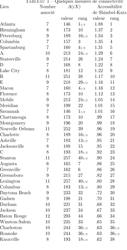
![Table 1 Some Measures of Connectiveness [134]](https://thumb-eu.123doks.com/thumbv2/123doknet/7411192.218260/17.892.191.652.205.1103/table-some-measures-of-connectiveness.webp)
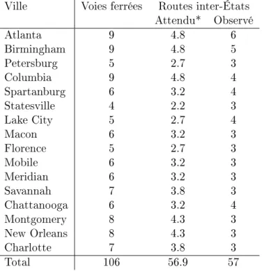
![Table 3 Comparison of Selected Cities [136]](https://thumb-eu.123doks.com/thumbv2/123doknet/7411192.218260/19.892.239.659.485.877/table-comparison-of-selected-cities.webp)


Documents relatifs
a) Un graphe est un arbre ssi il existe une chaîne unique entre chaque paire de sommets distincts. c) Un graphe G sans cycle, de n sommets et n-1 arêtes est un
En justifiant, associer à chacun des 4 nuages de points qui suivent l’un des coefficients de corrélation, ainsi que les séries étudiées :.. rang mondial des écoles de
Exercice 16 : pour chacun des exemples suivants, construire la matrice associée au graphe donné.. Exercice C : déterminer et utiliser une matrice d’adjacence On considère le
En effet, la relation d'équivalence entre graphes est transitive; en outre, le passage du graphe direct au graphe équivalent hiérarchisé (première proposition), puis du
En conséquence, dans un graphe simple non orienté, le nombre de sommets de degré impair est pair En effet, s'il existait un nombre impair de sommets de degré impair,
La conception de notre m´ ethode de s´ eparation et ´ evaluation progressive a ´ et´ e guid´ ee par une constatation : la borne inf´ erieure que nous pr´ econisons n´ ecessite
Le codeur est synchronisé avec une horloge clk de fréquence deux fois supérieure à la fréquence symbole, les données binaires entrante sont synchronisées avec clk et changent
Pour tout graphe G , χ(G ) = ∆(G ) + 1 si et seulement si G est un cycle impair ou un graphe complet (autrement, χ(G ) ≤ ∆(G )).. Th´
