Uiiiversité de IVlontréa.1
v1t/,
Une approche globale à l’estimation du mouvement de caméra pour des scènes encombrées
par
Viiiceut Cliapdelaine-Couture
Départemeut d’iuformaticiue et de recherche opérationelle Faculté des arts et des sciences
Mémoire présenté à la Faculté des études supérieures en vue de l’obtention du grade de lVlaître ès sciences (M.Sc.)
en Informatique
Octobre, 2004
D
Université
(111
de Montréal
Direction des bibliothèques
AVIS
L’auteur a autorisé l’Université de Montréal à reproduire et diffuser, en totalité ou en partie, par quelque moyen que ce soit et sur quelque support que ce soit, et exclusivement à des fins non lucratives d’enseignement et de recherche, des copies de ce mémoire ou de cette thèse.
L’auteur et les coauteurs le cas échéant conservent la propriété du droit d’auteur et des droits moraux qui protègent ce document. Ni la thèse ou le mémoire, ni des extraits substantiels de ce document, ne doivent être imprimés ou autrement reproduits sans l’autorisation de l’auteur.
Afin de se conformer à la Loi canadienne sur la protection des renseignements personnels, quelques formulaires secondaires, coordonnées ou signatures intégrées au texte ont pu être enlevés de ce document. Bien que cela ait pu affecter la pagination, il n’y a aucun contenu manquant.
NOTICE
The author of this thesis or dissertation has granted a nonexclusive license allowing Université de Montréal to reproduce and publish the document, in part or in whole, and in any format, solely for noncommercial educational and research purposes.
The author and co-authors if applicable retain copyright ownership and moral rights in this document. Neither the whole thesis or dissertation, nor substantial extracts from it, may be printed or otherwise reproduced without the author’s permission.
In compliance with the Canadian Privacy Act some supporting forms, contact information or signatures may have been removed from the document. While this may affect the document page count, it does flot represent any loss of content from the document.
Université de Montréal Faculté des études supérieures
Ce mémoire intitulé:
Une approche globale à l’estimation du mouvement de caméra pour des scènes encombrées
préseuté par:
Vincent Chapdelaine-Couture
a été évalué par un jury composé des personues suivantes:
Max Mignotte, président-rapporteur $ébastien Roy, directeur de recherche Douglas Eck, membre du jury
- 8 décembre 2004
RÉSUMÉ
Ce mémoire s’inscrit dans le domaine de la vision pa.r ordinateur, et plus précisément dans celui de la recherche automatique de la trajectoire de caméra à partir d’une séquence vidéo. La résolution (le ce problème peut mener à plusieurs applications dont la navigation autonome.
Nous analysons des vidéos de scènes encombrées. Ce type de scènes, composé d’une multitude d’objets à plusieurs profondeurs, survient fréquemment en milieu naturel (forêt, plantes, etc.) et en milieu urbain (câbles, salle remplie (le meubles, etc.) et sont propices aux occlusions et au problème d’échelle. Par conséquent, les méthodes traditionnelles de flux optique et de suivi de points sailla;its ne peuvent être appliquées sur ce type de scènes.
La séquence vidéo est transformée dans le domaine de Fourier spatio-temporel, puis analysée pour retrouver la trajectoire de la caméra. Une nouvelle méthode est établie pour l’analyse du mouvement latéral. Cette méthode est ensuite adaptée au mouvement global par rectification de la séquence vidéo. Son analyse ne nécessite ni décomposition en régions ni suivi de points saillants.
Mots-clés vision par ordinateur, neige optique, flux optique, problème d’occlu sions, problème d’échelle, analyse des composantes principales.
ABSTRACT
This thesis is a research in the field of computer vision and deals with egomotion
estimation from a vicleo sequence. Solving egomotion can lead tomany applications, like automated navigation for instaice.
We analyse videos of cluttered scenes, composed of many objects at clifferent depths (forest, plants, wires, etc.). Since scale and occlusion problems are severe in these scelles, traditiona.l optical flow methods cannot be applied.
A video sequence is transformed in the Fourier domain and a.nalvsed to estimate the camera motion. First, a new method to analyse lateral motion is presenteci. Then, the video sequence is rectified to estimate the global 3D motion. This analysis does not require the use of patches or tracking.
Keywords computer vision, optical snow, optical ftow, occlusion problem, scale
vi
RÉSUMÉ
TABLE DES MATIÈRES
iv
ABSTRACT
V
TABLE DES MATIÈRES LISTE DES FIGURES
• vi
ix
LISTE DES TABLEAUX
X
DÉDICACE xi
REMERCIEMENTS xii
INTRODUCTION
CHAPITRE 1 :TRAVAUX PRÉCÉDENTS
1
4
CHAPITRE 2 : NEIGE OPTIQUE
2.1 Algorithme pour analyser la neige optique 2.1.1 Cas particulier : absence de rotation 2.1.2 Cas général
z
9910
CHAPITRE 3 (ARTICLE) PRINCIPAL COMPONENTS ANALY
SIS 0F OPTICAL SNOW 12
3.1 Introduction
3.2 Previous work
3.2.1 Optical Slow
3.2.2 Bowtie axis estimation using wedge filter .
3.3 Bowtie Axis Estimation with PCA
3.3.1 Comparison of tlie two best fit plane methocÏs
12 13 13 16 18 19
vii
3.3.2 Pindillg the bowtie axis 21
3.3.3 Resuits 22
3.3.4 Comparhig the eigenvalues 23
3.4 Conclusioi 25
CHAPITRE 4 :ESTIMATION DE LA TRAJECTOIRE 3D DE LA
CAMÉRA 26
4.1 Méthode par décomposition de la vidéo e pièces 27
CHAPITRE 5 : (ARTICLE) A GLOBAL ANALYSIS 0F OPTICAL
SNOW FOR ARBITRARY CAMERA MOTIONS 30
5.1 IiitrocÏuctioii 31
5.2 Previous works 31
5.2.1 Optical Snow 31
5.3 Motion Field 34
5.3.1 IViotion Field Rectification 34
5.3.2 Finding rotatioll w 36
5.3.3 fiilding translation t 36
5.4 Experimeiltal results 36
5.5 Comparing the eigellvalues 37
5.6 Conclusion 38
CHAPITRE 6 :DISCUSSION 39
6.1 Algorithme biologiquement plausible pour l’analyse de la neige optique 39
6.2 Distribution d’énergie uniforme 39
6.3 Une approche hiérarchique 40
6.4 Analyse dans le domaine de Fourier des séquences rectifiées . . . 42
6.5 Mesure robuste de la présence d’un noeud papilloil 44
6.6 Distribution d’énergie des profondeurs 44
CONCLUSION . 48
BIBLIOGRAPHIE 49
ANNEXE I: PRÉSENCE D’ÉNERGIE SUR L’AXE DU NOEUD
PAPILLON 55
ANNEXE II: CODE DE L’ANALYSE DE COMPOSANTES PRIN
LISTE DES FIGURES
1 Exemples de flux observé lors d’un mouvement de caméra 2 2.1 Distribution d’énergie d’un noeud papillon dans le domaine de Fourier $ 2.2 Noeud papillon et prisme utilisé pour l’estimation de son orientation 10
2.3 Cisaillement temporel itératif 11
3.1 Wedge used to estimate the orientation of a howtie signature . . . . 15
3.2 Eigenbasis of a bowtie in the frequency domain 1$ 3.3 Sequences used to compare the Wedge method and the PCA method 23
3.4 fitness model of optical snow . . . 25
5.1 Eigenbasis of bowtie signature 33
5.2 Motion rectification 35
5.3 Sequences used to evaluate motion rectification 37 5.4 Fitness model of forward and lateral motions . 38
6.1 Distribution d’énergie avant et après normalisation . . 41
6.2 Exemple de l’effet de normalisation 41
6.3 Séquence test créée par professeur Richard Mann . . . 42
6.4 Exemple de l’effet d’un processus hiérarchique 43 6.5 Estimation de la distribution d’énergie des plans du noeud papillon 45 6.6 Estimation des plans limites du noeud papillon 46 1.1 Séquence Holly utilisée pour mesurer la concentration d’énergie sur
LISTE DES TABLEAUX
3.1 Comparison between the PCA method aiid the Wedge rnethod . 24
5.1 Motioii rectificatioii residts for synthetic anci rea.1 scenes 37 6.1 Étapes de l’analyse globale de scènes encombrées 47 1.1 Base propre en fonction du poids des énergies 56
xii
REMERCIEMENTS
Je veux tout d’abord remercier Sébastien Roy, mou directeur de recherche. pour m’avoir aidé à orienter ce projet et à l’approfondir par des discussions euri chissantes.
.Je remercie Michael Langer, professeur à l’université McGill, et Richard Manu,
professeur à l’université de Waterloo, pour leur disponibilité et leur précieuse col
lahoration ainsi que tous les membres du laboratoire d’informatique pour leur
soutien.
Je remercie également mes parents pour leur encouragement, et ma mère pour la lecture et la correction du texte de ce mémoire.
INTRODUCTION
Par ce qu’il voit, un observateur humain peut estimer son propre mouvement. Par exemple, en regardant par la fenêtre d’un train en mouvement, il peut évaluer sa trajectoire relative. L’objet de ce mémoire est d’estimer la trajectoire d’une caméra filmant l’espace environnant encombré d’une multitude d’objets à plusieurs profondeurs.
La trajectoire de la caméra et le mouvement d’objets dans une scène sont deux composantes importantes du mouvement observé clans une sécluence vidéo. Cepen clant, dans ce mémoire, nous ne considérons ciue le mouvement de caméra clans des scènes statiques.
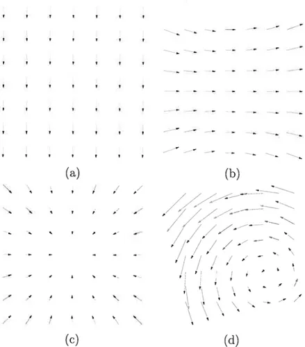
Le mouvement 3D de caméra génère un flux de mouvement 2D dans l’image (voir Fig. 1). IVIême si ce flux est connu, l’estimation du mouvement de caméra reste difficile puisclue chaque mouvement observé clans la sécluence dépend des paramètres du mouvement de caméra et de la profondeur de chaque point visible dans la scène.
Plusieurs approches existent pour l’estimation de la trajectoire de caméra. L’une de celles-ci estime directement le flux optique à chaque pixel à partir du gradient dans une séquence. Le flux optique est considéré depuis plus d’un demi-siècle comme un indice important utilisé par le système visuel humain [4]•
Cette approche suppose l’existence d’une vélocité unique à chaque point clans le champ visuel [3,44]
Cette supposition n’est cependant valide que s’il y a continuité dans l’espace, comme la surface d’un objet lisse. En effet, si un observateur se déplace devant une scène 3D encombrée, mie forêt par exemple, cette supposition n’est plus valide; les feuilles et les branches situées à plusieurs profondeurs causent beaucoup d’occlusions et des discontinuités du mouvement observé. Les frontières des nombreux objets présents dans la scène rendent donc difficile le calcul du flux optique. Or, on observe qu’une personne peut se promener facilement à travers des environnements 3D encombrés; des études psychologiques confirment d’ailleurs qu’un observateur humain peut s’oriellter dans tut nuage de points [1•
2 r t r r — r r r r (a) (b) / / ./ -0 — r » .. s » , -p » j A S P p r — Ø I A I \ t / t (c) (cl)
FIG. 1 — Exemples de flux observé lors d’un mouvement de caméra (a) Translation
vers le haut (a) Rotation vers la gauche (a) Tra;s1ation vers l’arrière ta) Trajectoire complexe.
3
Une autre approche se base sur le suivi de points saillants (coins, frontières, etc.). Cette approche robuste et rapide devient par contre difficile à utiliser pour des scènes encombrées clans lesquelles il y a une multitude de petits objets difficiles à suivre à cause des occlusions.
Récemment. Langer et Mann [1 ont introduit une nouvelle catégorie de mouve ments appelée neige opticue. La neige opticue généralise le flux optique en aban donnant toute contrainte de continuité spatiale. Les scènes de neige optique (ou
encombrées) sont composées par définition de petits objets situés à une multitudede
profondeurs. Comme mentionné précédemment, si lon abandonne la contrainte de continuité des profondeurs, les méthodes traditionnelles de flux optique ne peuvent plus être utilisées. La neige optique fournit d’importants indices sur la profondeur et le mouvement, et s’avère particulièrement utile au calcul de la trajectoire de
caméra.
Nous estimerons. clans ce mémoire, la trajectoire de caméra en utilisant les principes de la neige optique, sans calculer le flux et sans suivi de points saillants. Au chapitre 1, nous ferons une revue des principaux travaux s’inscrivant dans le domaine de l’estimation du mouvement de caméra. Puis, au chapitre 2, il sera question des principes de la neige optique établies dans les travaux des professeurs Langer et Manu. Nous présenterons, au chapitre 3, un algorithme pour résoudre rapidement le modèle de neige optique en utilisant l’analyse des composantes prin cipales (PCA). Au chapitre 4, nous résumerons les travaux reliés à l’estimation de la trajectoire 3D de la caméra pour des scènes encombrées. Soulignons que ces tra vaux proposent une analyse des mouvements latéraux par régions, alors que nous présentons, au chapitre 5, une rectification de la séquence origimiale qui permet une estiniation rapide et globale du mouvement arbitraire de caméra pour des scènes encombrées. Cette approche ne nécessite aucune décomposition en régions. Nous terminerons par une discussion au chapitre 6, qui sera suivie d’une conclusion.
CHAPITRE 1
TRAVAUX PRÉCÉDENTS
Ce chapitre résume les travaux reliés au problème de l’estimation du mouvement de caméra, excepté les articles ayant servi de base pour ce mémoire et qui feront Fobjet des chapitres 2 et 4.
Plusieurs méthodes de vision par ordinateur ont été développées pour analyser la trajectoire du mouvement de caméra. Des hypothèses sont habituellement as sociées au modèle de la trajectoire de caméra ou au modèle de l’environnement. Par exemple. Adiv a supposé un modèle simplifié du monde, composé de sur faces planaires; Horn et Weldon t15[ ont limité l’espace des mouvements possibles (translation pure, rotation pure, ou trajectoire générale avec profondeur connue) Fleet et Jepson [16]
ont supposé la constance temporelle d’un mouvement sur une longue séquence. D’autres méthodes [17—19] utilisent une analyse spatio-temporelle pour estimer les vélocités locales d’une image avec de larges régions temporelles.
Le mouvement 3D de la caméra est souvent estimé à l’aide du flux optique ou du flux normal (flux optique clans le sens du gradient de l’image) dérivé à partir de deux images [14, 20,22-30] ou à l’aide de la correspondance entre des points saillants préalablement détectés d’images successives [3133] Ces deux approches dépendent de la texture dans l’image et de la précision des étapes de prétraitement [[. Le calcul du flux normal est plus précis que celui du flux optique, mais son analyse est plus ambigué. De plus, le calcul du flux optidlue dépend de la continuité spatiale dans la scèneS. Cette hypothèse n’est plus valide pour des scènes encombrées. Quant aux points saillants, ils peuvent être détectés sur un plus long intervalle de temps en utilisant des filtres temporels récursifs ]16]• IViais le problème de repérage de points saillants utiles et celui des occlusions persistent.
Plusieurs auteurs [15,35.36]
proposent de calculer la trajectoire de caméra clirec tement à partir de l’intensité des pixels. Horn et Weldon [151 analysent seulement
des cas particuliers, comme décrit précédemment. Haima [35]
5 itérative pour des cas généraux, mais requiert une approximation initiale raison nable. Taalebinezhaad [36]
a dérivé une formulation mathématique complète, mais s’appuie sur des calculs à partir de points d’ancrage de même intensité entre cieux images, ce qui peut être très instable.
Les rotations et les translations 3D induisent des images 2D similaires ce c1id cause des ambigiiftés d’interprétation, particulièrement lorsqu’il y a présence de bruit. Retrouver le mouvement de caméra 3D à partir du flux optique est un problème mal posé puisque de petites erreurs dans le flux optique 2D peuvent cau ser de larges perturbations clans le mouvement 3D obtenut371. Par contre, il est beaucoup plus facile de distinguer les effets de rotations et de translations 3D aux discontinuités de profondeur, puisque le mouvement 2D de pixels rapprochés à des profondeurs différentes a des composantes rotationnefles très similaires, mais des composantes translationnelles très différentes [40[•
À
partir de cette observation, des méthodes utilisant la parallaxe de mouvement ont été construites pour obte nir la trajectoire 3D de la caméra [20,33, 40—42]Il est intéressant de noter que les discontinuités de profondeur donnent beaucoup d’information pour distinguer les composantes transiationnelles et rotationelles, mais que le flux optique y est plus difficile à calculer. Dans [20,40[
différents vecteurs, calculés à partir du flux optique, annulent les effets des rotations, et le point d’expansion (FOE focus of expan sion, l’intersection entre le plan image et la direction de la composante translation du mouvement de caméra et l’image) est obtenu à l’intersection de ces vecteurs. Cependant, les ciiscoiitinuités de profondeur rendent le flux optique très imprécis, affectant ainsi le calcul de la parallaxe de mouvement.
Heeger[12]
utilise des filtres de Gabor pour une analyse dans le domaine fréquentiel. La méthode repose sur la propriété qu’une région à profondeur constante subissant une translation produit un plan d’énergie dans le domaine fréquentiel.
Récemment, Langer et l\/Iann [7,9]
ont introduit une nouvelle catégorie de mouve ments appelée neige optiquedans laquelle aucune continuité spatiale n’est supposée. Nous utilisons, dans ce mémoire, les principes de la neige optique pour estimer le mouvement de caméra. Notre méthode ne reciuiert aucun suivi de points saillants
6 et aucuue décompositiou en régions. Puisque l’analyse se fait dans le domaine de Fourier, nous supposons une constance temporelle du mouvement de caméra d’une longueur choisie par l’utilisateur, c’est-à-dire que le mouvement de caméra doit demeurer constant pour un nombre T d’images consécutives.
CHAPITRE 2
NEIGE OPTIQUE
Ce chapitre introduit le modèle de neige optique permettant l’analyse de scènes encombrées. Dans de telles scènes. aucune continuité spatiale nest supposée et plusieurs vélocités peuvent être perçues aux environs dm pixel. Les méthodes traditionnelles cïestimation du flux optique ne sont clone plus valides. De plus. les scènes encombrées contiennent un grand nombre d’occlusions, ce qui rend le suivi de points saillants très difficile, voire impossible.
Les principes de la neige optique [7,9]
sont une extension de la propriété d’un plan en mouvement [51 qui énonce qu’une région de la scène de profondeur constante subissant une translation latérale (c’est-à-dire perpendiculaire à l’axe optique) de vélocité (y1,v.O) produit un plan dans le domaine de Fourier.
De façon pius formelle, soit I(x,y,t) une séquence d’images. Si une région de la séquence subit une translation pure de vélocité (u1, un), nous savons de [z15[
que cette vélocité est contrainte par
ai
ai
aï
(2.1) 8y
at
La transposition de cette contrainte dans le domaine de Fourier produit l’équation suivante
—2(v1f1 + v9f + f)Î(J1,
f, f)
= 0 (2.2)où
Î(f1, f,
ft) est la transformée de Fourier de I(x, y,t). L’équation 2.2 implique que toutes les fréquences non nulles deÎ(x,
y,t) sont sur le planu1f1+vf+J O. Dans [7, 9], ce modèle a été étendu à la situation où un ensemble de vélocités ont un paramètre libre à l’intérieur d’une région, c’est-à-dire où les vélocités varient8 selon l’équation
(y1,v) = (u, + at1, u + at) (2.3)
où ‘u.‘un. t1 et t sont des constantes et n est une variable inversement propor tionnelle à la proforcleur visible au point
(,
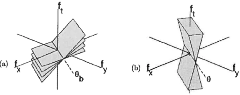
y). Comme décrit plus en détails au chapitre 4, ‘ui, sont reliées à la rotation de la caméra et t, t, à sa translation.Ce nouveau modèle porte le nom de neige optique et produit plusieurs plans clans le domaine frécluentiel. Ces plails forment un noeud papillon (voir figure 2.1) qui respecte les deux propositions suivantes
Proposition 1 Les plans du noeud papillon sintersectent en une ligne, appelée l’axe du noeud papillon, passant par l’origine.
Proposition 2 L’axe du noeud papillon suit la direction (—tu, t1, u1t—v9t1).
En normalisant le vecteur (t1, tu), cette direction devient (—ta, t1, U sin(O)), OÙ O est l’angle entre les vecteurs et (n1,n).
FIG. 2.1 — (a) Distribution d’énergie dans le domaine de Fourier (a) d’un point
de vue perpendiculaire à l’axe du noeud papillon (h) d’un point de vue parallèle à l’axe du noeud papillon.
La neige opticlue ne suppose aucune continuité spatiale, contrairement aux modèles standards de mouvement comme le flux optique ou le mouvement en couches. Le modèle de neige optique permet donc de grandes discontinuités de profondeur. En fait, l’ouverture du noeud papillon s’agrandit en fonction de qui
9 s’il n’y a qu’une profondeur visible, le noeud papillon devient un simple pian et la notion d’axe ne tient plus.
Puisque les deux premières composantes de l’axe du noeud papillon donnent la direction de la translation, cet axe permet donc de séparer les composantes rotationnelles et translationnelles du mouvement. Sans cet axe, ces composantes sont confondues.
2.1 Algorithme pour analyser la neige optique
Langer et Manu [9] ont tout d’abord développé un algorithme pour trouver l’orientation du noeud papillon pour une trajectoire de caméra sans composantes rotationnelles u et ut,. Cet algorithme a ensuite été modifié dans [6]
pour permettre la présence des composantes rotationnelles.
2.1.1 Cas particulier absence de rotation
Langer et Mann [9] ont développé un algorithme pour trouver l’orientation du noeud papillon dans le ca.s où u1 = O (c’est-à-dire aucune rotation), ou lors du
suivi d’un point dans la scène, c’est-à-dire lorsque le vecteur (—u9,
u1)
est parallèle au vecteur (t1, t9). Dans ces deux cas, l’axe du noeud papillon repose dans le plan de pente(f1, f9,
O) en direction de (—tu, t1, O).À
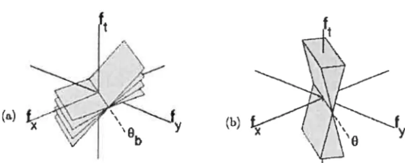
partir du spectre des puissances l’algorithme développé dans [9] profite de la géométrie du noeud papillon. L’orientation de l’axe du noeud papillon corres pond à l’angle qui accumule le moi;s d’énergie dans un prisme à base triangulaire de pente Vmax (voir Fig. 2.2-b). L’énergie minimale, nulle en théorie, se trouve en pratique affectée par les effets de frontières (exemple d’effet de froitières).Plus précisément, pour un angle O, Langer et Manu [9]
définissent
fo
comme suit:‘o
ft
(a) f
X ‘ )
f
bFIG. 2.2 (a) Noeud papillon dans le domaine fréquentiel. L’axe du noeud papillon est dans la direction &. (b) Prisme utilisé pour l’estimation de l’orientation du noeud papillon.
Soit T le nombre d’images dans la séquence et N la taille des images. L’énergie est accumulée suivant la condition < V,
De plus, pour s’assurer que l’énergie accumulée minimale soit de O, Langer et Mann [9] n’utilisent que les fréquences qui satisfont
f(fo, ft)ff2
>r
en raison del’imprécision de la vélocité des basses fréquences.
Avant d’effectuer la transformée de Fourier, l’intensité moyenne de la séquence est soustraite de la séquence originale pour enlever la composante continue (le DC). Un fenêtrage Gaussien de la séquence originale, d’un écart type d’un sixième de la taille de l’image, est aussi appliqué à la séquence pour réduire le bruit dû aux effets de bord dans le domaine de Fourier.
2.1.2 Cas général
Dans le cas où il y a présence de rotation, l’axe du noeud papillon ne repose
plus dans le plan de pente
(f f9,
O). Maun et Langer [6]utilisent une compensation de mouvement [46] pour annuler l’effet de la rotatioii. Pour ce faire, il faut trouver un plan rr = (m’, mb,, 1) qui minimise la somme des différences
ffÎ(h,f9,(ft-mJ-m9f9)
mod M)f2.(f,f,ft)NxNx M
Une fois ce plan estimé, les puissances sont déplacées suivait l’axe
f
d’une11
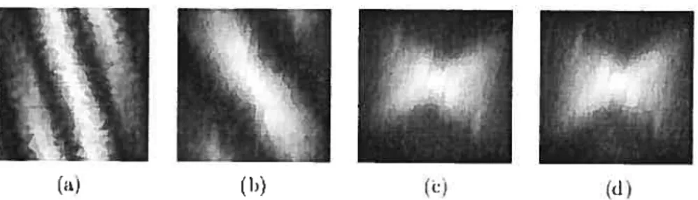
FIG. 2.3 Processus du cisaillemellt temporel itératif, des puissances origmales en ta) aux puissaices complètement cisaillées en (cl). On petit clairemellt voir e (a)
l’aliassage temporel causé par les pentes trop abruptes des plans.
plail de pente
tf f,
O), c’est-à-dire ayant comme iormale (0, 0, 1) (voir Fig. 2.3). Puisque tous les piais du noeud papillon contiennent l’axe du noeud papillon, le plan ir contien aussi l’axe du iioeud papillon et l’axe repose donc dans le plant f, f,
0). L’axe du ioeud papillon peut ensuite être trouvé à l’aide de la méthodedécrite à la section 2.1.1.
La composante rotationnelle ;ormale û est ensuite calculée selon l’équation
= m — (m
où ‘f est la direction trallslatiomielle retrouvée à partir de l’axe du lloeud pa pillon et m (m’,mL,).
Nous présentoils dans l’article qui suit une nouvelle méthode basée sur l’analyse des composantes principales permettant l’analyse rapide de la neige optique dans
le cas général et ne nécessitant aucun paramètre.
1
CHAPITRE 3
(ARTICLE) PRINCIPAL COMPONENTS ANALYSIS 0F OPTICAL SNOW
Cet article [63]
a été publié comme l’indique la référence bibliographicue V. C-Couture, S. Roy, M. S. Langer et R. Mann. “Principal Components Ana lysis of Optical Snow” dans British Machine Vision Con ference 2004 (BMVC’04), Kingston (UK), septembre 2004, vol. 2, pages 799-808. L’article est présenté ici clans sa version originale.
Many applications in computer vision use Principal Components Analysis (PCA), for example, in camera calibration, stereo, localization and motion estimation. We present a new and fast PCA-based methocÏ to analyze optical snow. Optical snow is a complex form of visual motion that occurs wheii an observer moves through a highly cluttered 3D sceiie. For this category of motion field, rio spatial or depth co herence cari be assumeci. Previous methods for measuring optical snow have used a wedge filter in a spatiotemporal frequency domain. The PCA method is also based on the spatiotemporal frequency domain analysis, but examines a differellt geome
try property of the spectrum. We compare the results of the PCA method to the
previous methocis using both real and synthetic secluences.
3.1 Introduction
Recently, Langer and Mann [7]
considered a category of visual motion called opticat snow which generalizes optical flow by abandoning classical assumptions of spatial continuity. Optical snow arises when an observer moves relative to a rigici 3-D cluttered scee or object (falling snow, forest, plants). Optical snow is characterized hy small spatial features and a dense set of depth discontinuities. It procÏuces a highly discontinuons motion fielcl. Traditional optical flow methods
13
camiot be expected to recover an image velocity field from optical snow since these methods tvpically assmne local snioothness in the velocity field 1, or a small num
ber of weÏl-isolated discontinuities e.g. [53—55] definition. smoothness constraints
do not apply for optical snow. Layered motion models sucli as 113, 57-61 also do not
apply, since these models assume smoothness within layers[56l, and the number of layers is typically very small (2 or 3). In optical snow, the number of “layers” can be in the hundrecis or more.
To overcome the dense depth cÏiscontinuity problem that arises in measuring optical snow, Langer and Mann 1’ introduceci an analysis of the motion which was hased in the spatio-temporal freqnency clomain. In [8,9[, they presented an
algorithm to find the direction of the motion for the special case of parallel optical snow, which arises for example in the case of a lateral camera motion [8,61] This
algorithm was then generalized in [6]
to handie the case of optical snow that arises from general observer motion, including both non-lateral motion ancl camera roil.
The previous method for measuring optical snow uses a wedge-filter to estimate the distribution of power in the spatio-ternporal Fourier power spectrum. This filter was rnotivated hy the geometric properties of optical snow in the spatio-ternporal frequency domain (see Sec. 3.2). In this paper, we present a new and fast algorithm which uses PCA to estimate the properties of optical snow. The PCA method is complementary to the wedge filter method, in that it is based on a geometrical property of the power spectrum that the wedge method ignores. We show the effectiveness of the PCA method by comparing experimental resuits of the PCA method to that of the wedge method of [9]
3.2 Previous work
3.2.1 Optical $now
Optical snow is produced by an observer moving relative to a rigid 3D cluttered
scene. It is a special case of motion paraltaxin which the density of clepth disconti
14
image velocity field can be closely approximated as a sum of two fields — one that
is due to camera translation and the other due to camera rotation [2J As a resuit,
the image velocity vectors in a local image patch satisfy the relation
(vx, v) = (n + ù t, ‘u. + t) (3.1)
where ‘ut, u,, t, t are constants which depend on the patch and c clepencis on
position x, y in the patch and on the depth of the point visible at (x, y) [6]•
Thus,
optical snow vielcls a 011e parameter family of velocities (a une!) in any local image patch.
Que can examine the power spectrum properties of optical ftow by using Eq.
(3.1) to extend the classical motion plane property 5,12J The motion plane property states that an image transiating with uniform image velocity produces a plane of
energy in the 3D spatio-temporal frequency domain. Formally, let I(x. y, t) he a time varying image which is defined by an image patch transiating with velocity
(v, va). From [41, this velocity is constrained hy
ai
ai
ai
(3.2)
This constraint, transposed in the Fourier domain, yields
(vf+vfy+f)
Î(J,f.f)
0 (3.3)where
Î(J, f,, f)
is the Fourier transform of I(x,y, t). Eq. (3.3) implies that all frequencies(h f,
ft) for whichÎ(f, f, f)
O lie on the planev1f1 + vf9 + ft = 0. (3.4)
Substituting Eq. (3.1) into Eq. (3.4) yields a family of planes in the frequency cloinain,
15
This set of planes forrns a bowtie (see Fig. 3.la) and follows the two following propositions [9]
Proposition 1 The planes of the bowtie intersect at a common une, called the
aris of the bowtie, that passes through the origin.
Proposition 2 : The axis of the bowtie is in direction (—t9,t,, n,t9—n9t,) in the 3D frequency domain. By normalizing (t,, t1), this direction becomes (—t9, t,, UJ sin()), where is the angle between vectors (t,, t9) anci (n,,‘tt9). By assuming that (t,, t9)
is perpendicular to (u,, n9). we get (—t9, t,. \/‘Li; + n
).
For simplicity, ail equations in this paper assume image sequences of equal dimension in space and time, i.e. the size N of image region equals the number T of frames. In practice, the case of unequal dimensions can be easily be accounted for using factors of
‘vVe emphasize that optical snow is a very general moclel of visual motion. It
clescribes the velocities of any rigid 3D scene as seen hy a moving observer [6,1
The model applies whether the surfaces are partly transparent, smooth, layered, or densely cluttered. The model does not assume any spatial continuity. This is in sha.rp contrast to conventional optical fiow estimation which relies on spatial coherence of the motion fields or uses motion layers model.
ta)
(b)
FIG. 3.1 — (a) Bowtie signature in the frequency domain. The axis of howtie is in
direction &. (b) Wedge used to estimate the orientation of the howtie. The dotted une at angle O in the
(f,, f,)
is denoted 1.16
3.2.2 Bowtie axis estimation using wedge filter
Langer and Manu introduceci an algorithm to find the howtie axis in the case that (ut, u) = (O, O), where no rotation is allowed. In this case, the bowtie
axis lies in the
(f, f,
O) plane and the direction of the bowtie axis is (—tu, t, O).To find the bowtie axis, a wedge fitter is used. The wedge filter is defineci by two
motion planes, of siope +VmaT, respectively. These two planes intersect at a une in the
(f,
fi,) plane, which is oriented at an an angle O (see figure 3.1). We lett denote this une. It corresponds exactly to the axis of the bowtie when O =
If all motion planes in the bowtie have siopes of magnitude that is less than then, for this O, the intersection of the weclge filter and the howtie will be restricted entirely to the bowtie axis.
To find the bowtie axis, the wedge filter is rotateci (O is varied) and the power
that falis within the weclge filter is measurecÏ as a function of O. In particular —
and this is an important cletail a small cylinder containing the line i is removed from the wedge filter. This removes all power from the wedge filter for the case that O = °b The angle °b of the bowtie axis is estimated to 5e the angle for which the power in the wedge filter is a minimum.
The more general case is that (ut,‘un) (0, 0). In this case, the howtie axis does not lie in the
(f J)
plane (see Proposition 2). To estimate the bowtie axis in this case. a methoci vas presented in [6jThis method fias two steps. The first step is to find the best fit motion plane for the bowtie and then shear the power spectrum in the ft direction to bring this motion plane in correspondence with the
(f f)
plane. This shear amounts to motion compensation [46] of the imagesequence (within the patch in question) such that the mean velocity in the patch becornes 0. In particular, since the bowtie axis is contained in ail motion planes within the bowtie, this best fit plane also contains the bowtie axis. The second step
of the rnethod for finding the bowtie is to find the O that best aligns the wedge
filter to the bowtie, as described ahove for the case that the bowtie axis happens to already lie in the
(J f0)
plane.17
To perform motion compensation, Maun and Langer [6] find the vector
(v,v)
that miiximizes the 5um of squares
g(vx, v) = Î(fT,
J
ft) 2(f
— (VTfX +e2!2) mod N))2 f f ,ftWe Te-express the motion compensatioi step, iII a way that xviii aliow us to compare
it to the PCA method. which xve introduce in this paper.
Let F 5e the 1V3 x 3 matrix which lists the N3 possible frequency triplets
(f, f2,
ft), where eachf,
ft value is in {O,. . . ,N — 1}.
Let ‘W 5e an N3 x N3diagonal matrix of weights, with diagonal elements,
W(f1,
J, f)
=Î(f f’ LH.
Consider the matrix procluct
Zf
W(f,f2,f)2f1 f
W(J,f,f)2f
W(J,f,J)2FTW9F
Zff2
W(f,f2,f1,)2Zf
W(J.f2,f)2Zf2
Jt T1’(J.,fy’ft)2ZJf
l1(J,f2,f1)2 JJ2 14(Jx,fy,ft)2ZJ?
W(fx,fq,Jt)2where each of the summations is a triple summation over
f, f,, f,
namely over the entire 3D frecuency domain. In tlie case that there is no temporal ahasing, the modulus N can 5e ignored and the summation is equivalent tog(vx, e2) (vs, v, —1) FTV2 F (v,vy, 1)T
This inethod thus finds the best fitting motion plane by miuimizing the weighted squared distance in the ft direction.
With this hackground, let us noxv turn to the original contribution of this paper which is to introduce a new, simpler and faster PCA-method for findling the howtie axis.
‘s
3.3 Bowtie Axis Estimation with PCA
The basic idea of or PCA methocl is to finci a une in the frequency dornain
that passes through the origin and contains a concentration of power. It does so
by computing the eigenvectors of a 3 x 3 covariance matrix which is defined in the
(h’ f.
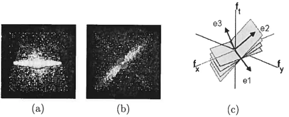
ft) domain. This strategv is justified bv the fact that the eriergv on thebowtie axis is the superposition of the energies (not merely the intersection) of the planes that contribute to the bowtie (see fig. 3.2).
e3
(
el(c)
FIG. 3.2 — (a) Energy distribution in the Fourier domain from a viewpoint perpen
dicular to the axis of the bowtie (b) Energy distribiltion in the Fourier clomain from a viewpoint parallel to the axis of the bowtie (c) Eigenhasis of bowtie signature.
The PCA methoci uses classical orthogonal distance regression [1],
which fincis the best fit line and best fit plane to a set of 3D points. In our problem, the 3D space is the frequency domain and so the coordinates are
(f’,
fi,, ft). The unes and planes we are interested in pass through the origin. Letn,f + nf + nf = O
be the equation of a plane that passes through the origin, where
nT = (n n, nt)
19
weighted distances of each
(J, f, f)
to this plane,f(n) Wth,f,J)2 n
f
+ nf
+f.f.ft
The function f(n) eau be expressecl as the matrix product
j() (T FT W2 F )/(T)
where F is the same matrix asiii Sec. 3.2. We vill cliscuss our choice of T/V(f,
f,
ft)below.
The function f(n) is a Rayteigh quotient. This quotient is maximized and mi nimized by the eigeuvectors corresponding to the largest smallest eigenvalues of
FTV2F, respectively. The minimum eigenvector defines the normal of the best fit
plane n. The maximum eigenvector clefines to the best fit une t which is considered to be the bowtie axis. The Hue t aiways lies in the plane n, sirice FTW2F is a
symmetric real 3 x 3 matrix and so it has an orthogonal set of eigenvectors. 3.3.1 Comparison of the two best fit plane methods
Both the wedge filter method of [6,9]
and our new PCA method compute a minimization which finds a motion plane that best fits a bowtie. However, there are several differences between the methods.
Let us first hriefiy mention two minor differences. Que is that f(n) measures the weighted distance orthogonal to a plane, whereas g(vx, u9) measures the weigh
teci distance in the ft direction only. Que eau make arguments for either of these
distance choices. Indeed similar non-orthogonal [12,62] vs. orthogonal [50,52]
choices were made in classical optical fiow. A second difference is that the f(n) minirni zation normalizes by the length of n, whereas the g(v1, u9) minimization does not normalize by the length of (v, u, —1). The effect of normalizing is to explicitly penalize for high speeds. Again, arguments eau be made for or against.
20
For wedge filter method [6],
the weighting furlctioll was the amplitude spectrum
Î(f,
fy,f)
. The amplitude spectnim turus out to be inappropriate for the PCAformulatioll, however.
To uiiderstand how problems can arise, consider au illustrative example. Sup pose that an image sequence is clefined by summing two transiating image sequeices
I(x,y.t) Ii(x,y,t)+I2(’,yt)
The Fourier trarisform of the summed image sequence is
î(f1, J, f)
=Îi(f, f, f)
+ fy,J)
with power spectrum
Îtf,f,f)
2= j
Î1(f,f2,f))
2 +Î2(f,f2,f))
2 + 2 Re(Îi(ff2ft) Î2(f,f2,f)).
Let’s consider the expected value. The phases of
Î1(f f2, f)
and 12(fT,f, f)
eau be assumed independent, so we haveE
{
Î1(f, f9,
fi)Î2(f. f9, f) }
=0and 50
21
The expected power spectra On the bowtie axis is thus the sum of the expected power spectrum of the two component image sequeilces. Thus there is a coilcentra tioll of power 0n the bowtie axis, which is where the two planes superimpose.
Unfortunately, there is 1IO reason why the PCA method should cletect this
concentration of power, if we choose W(f,
f,, f)
I(fr,f, f)
as does the wedge method. To illustrate, take the counter-example in which the first frame (alld heilce ail frames) of the two transiating images have the saie amplitude spectra,Îi(f f)
=f2(f,
j,) , but they have independent phase spectra. Further suppose that two transiating images sequeces have equal but oppo site velocities. Theu oie ca show that two of the eigenvectors of FTW2F lie in
the plane
(f f,)
and the third eigenvector is parallel toL.
iVioreover, the direc tioll of the two eigenvectors in(f f,)
depends on ouly on the amplitude spectra.I
Îi(fx,fy) = 12(Jx,f,)
. These eigenvector directions would be ilKlepenclellt of the direction of image motion. Thus, for this comlterexample, the PCA method would not he able to recover the bowtie axis, eve though there is a concentration of power there. We have done experiments to show that this difficulty arises for more general sequeces (voir l’annexe I).3.3.2 Finding the bowtie axis
The difficulty that we just described arises hecause the power spectrum is a se colld order property, whereas the conceiltration of power that occurs on the bowtie axis is a higher order property. This difficulty is avoided by using a higher order power of the Fourier coefficients, namely
22
Running a similar argument as above on the expected values yields
E
{ I V(ff2f)
2 E{I
Î(f,f2,J)
41
= E{ (I
Ii(J,f2,f)) 2 + 12W.fy,Jt) 2 + 2 Re(f1(h.. f2.
ft)f2(f,f9.
ft)) )
2 = E{ I
fi(f1,f2,f))I}
+E{ I
f(f,fy,ft))I
+ E{
4 (Re(Îi(f,f2f) f9(ff2f)
)2}
+ E{
2f(f,f2,f2
f2(f,j2,f) 12}
+ E
{
2 Re( fl(JT,fy,ft) I2(f,f2,f))(11i(fr,fyit)
2+ I2(f,f2,ft) 2)
}•
The first four terms in the summation are all positive, whereas the last term vanishes, since Re(
Ii (f,
ft) I.2(J,f,, f) )
is equally likely to be positive as negat ive.In particular, we observe the desired interaction of the two motion planes along the bowtie axis. There, the third and fourth terms in the summation are positive since both I1(f,
f, f)
andI9(f, f2, f)
are simultaeously non-zero and each of the terms involves squarecÏ (and hence positive) quantities only. These ternis add a large extra weight to the minimization, which causes the first eigenvector e1 of FT W2 F to align with the bowtie axis.3.3.3 Resuits
To evaluate our method we rendered several synthetic image sequences of scenes
containing lambertian spheres (see Fig. 3.3). Image motion was generated by mo
ving a camera (45° field of view) through the scene with varions translation and rotation parameters. For taterat camera motion (axis of translation and axis of ro
tation both perpendicular to the optical axis) and a srnall field of view, the motion satisfies Eq. (1) and a bowtie should be present.
23
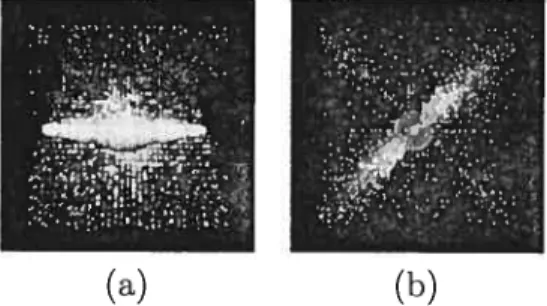
FIG. 3.3 — (a) Synthetic scenes consisted of small halls at a wide range of clepths (64
frames of size 128x128 pixels). (b) Holly bush taken from a horizontally transiating camera (32 frames of size 64x64 pixels). (c) Lab sequence taken from a camera transiating diagonally in the image plane (40 frames of 128x128 pixels).
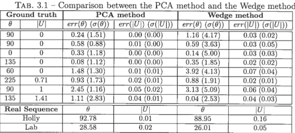
for the real sequences in the last two rows, each row shows the average over ten mus of each method. We report both the error anci the standard cleviation u of estimated bowtie parameters O and U =
Jn
+v..
We use both synthetic and real scenes to compare the accuracy of the PCA method to the wedge-based method of [6,7,9] The resuits are very similar. Temporal shearing (see Sec. 3.2.2) is used as a preprocessing step of the PCA method to account for temporal aliasing. We also perform a power normalization 021 for each spatial frequency(f. f)
to ensureuniform power distribution. Note that the PCA method is parameter-free. The wecÏge method lleecls two parameter, the siope of the wedge Umax and the cylinder
radius
r
(sec Sec. 3.2.2). For ail sequences, Umax was set to 1.0, except for the hollysequence, where 2.0 was useci. A radius r of 4 pixels was used in ail cases. These values are somewhat image dependent, which emphasizes the acivantage of getting rid of pararneters.
The average running times for the wedge method was 30seconds’. Under similar conditions, the PCA method muns in arounci 1.5 seconds.
3.3.4 Comparing the eigenvalues
Although scenes with a wide range of depths often produce optical snow, there are certain conditions in which opticai snow does not occur. The flrst example
(a) (h) (e)
24
TAB. 3.1 — Comparison between the PCA rnethod and the Wedge method
Ground truth PCA method Wedge method
L1
U err(8) ((9)) err(IUI) (u(IUD) err(8) (a(9)) err(IUI) (u(IUD) 0 0.24 (1.51) 0.00 (0.00) 1.16 (4.17) 0.03 (0.02) ïii5 0 0.58 (0.88) 0.01 (0.00) 0.59 (3.63) 0.03 (0.05) ii 0 0.33 (1.18) 0.00 (0.00) 0.14 (5.00) 0.03 (0.03) 0 0.08 (1.12) 0.00 (0.00) 0.35 (1.85) 0.02 (0.02) 0 1.48 (1.30) 0.01 (0.01) 3.92 (1.13) 0.07 (0.04) 0.71 0.93 (1.73) 0.02 (0.01) 0.88 (1.91) 0.02 (0.01) 1 2.45 (1.16) 0.05 (0.02) 3.13 (5.09) 0.06 (0.04) 135 1.41 1.11 (2.83) 0.04 (0.01) 0.04 (2.53) 0.01 (0.03)Sequence &
I
lUI
9 lUIHolly 92.78
J
0.01 88.95 0.16Lab 28.58
J
0.02 26.01 0.05is if the objects are ail distant (a mountain seen hy a walkiiig observer) then the translation compollent of the image velocities vanishes, since the translation component depends n inverse depth [2J Second, even if the objects are nearhy, if the observer is moving directly forwarcl and the field of view is small, then the translation component of image motion is small. The reason is that the translation
component varies directly with the angular distance from the direction of heading. Third, if the camera motion is pure rotation (notranslation), then the image motion fieÏd is indepenclent of depth. In ail three of these cases, the “bowtie” in fact consists only of a single motion plane.
When only a single motion plane is present, it is the best fitting plane to the “bowtie”. This plane ir is spanned by the eigenvectors e1 and e2. The eigenvalues would depend 011 the spatial orientation structure in the (transiating) image, rather
than on a bowtie axis. Moreover, the eigenvàlue for the e3 direction would be near zero.
With this issue in mmd, we would like to estimate 110w well the analyzecl motion corresponds to optical snow, i.e. if a bowtie is present. We define a howtie “fitness measure” by comparing the two largest eigenvalues. There are two extreme cases to consider. The first is that optical snow is present and there is a wide range of image speecÏs. In this case, the first two eigenvalues should correspond to the bowtie axis and a perpendicular vector in the best fitting plane ir, respect.ively.
25
The second extreme case is that a single motion plane is present. Assuming that spatial content of the image is roughiy eveiiiy distributed over ail orientations. the two corresponding eigenvalues should be equal.
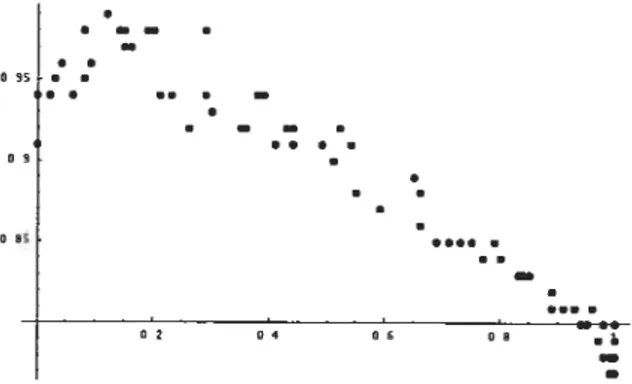
figure 3.4 shows a plot of the ratio of the ftrst two eigenvahres À2 and À1 as a function of the range of depths. As predicteci, the ratio falis off as the range of cÏepths clecreases.
035
03
005
— 02 04 06 08
FIG. 3.4 — as a function of depth range (from a single depth to a large interval).
As expected, it starts at 1 (pure plane) and decreases as a bowtie signature takes shape.
3.4 Conclusion
We presented a new simple PCA-based method to analyze optical snow. The performance of the rnethod in estimating the bowtie axis is similar to that of the previous method, which is based on a wecige ifiter. As the resuits clemonstrated, the PCA niethod lias many acivantages such as its simplicity, its efficiency and its absence of parameters.
CHAPITRE 4
ESTIMATION DE LA TRAJECTOIRE 3D DE LA CAMÉRA
Ce chapitre traite du problème de l’estimation du mouvement 3D de caméra pour des scènes encombrées. Le mouvement de caméra est régi de façon générale par six paramètres, soit les trois composantes translationneÏles t, t,t et les trois coin posantes rotationnelles w, w,,w. Pour une scène rigide, le mouvement perçu par la caméra dépend de sa trajectoire et des profondeurs clans la scène. Le modèle de neige optique, décrit au chapitre 2, est en mesure d’analyser des scènes encombrées caractérisées par mie multitude de petits objets à différentes profondeurs. Comme décrit précédemment, les méthodes standards de flux optique et de suivi de points saillants (tracking) sont inadéquates pour de telles scènes. Nous avons présenté, au chapitre 3, une nouvelle méthode d’analyse des composantes principales du modèle de la neige optique.
Pour estimer le mouvement de caméra 3D dans un cadre général à l’aide de ce modèle, deux approches sont proposées. Premièrement, l’approche locale se base sur le fait ciue plus une région est petite et plus le mouvement, au départ 3D, devient approximativement latéral et 2D. Pour une région i, l’équation 2.3 de la neige optique devient
(v, v) = (Wj + at,Wj,, + ct) (4.1)
où w.W) est l’approximation locale de la rotation de caméra et tir,Ç, l’ap proximation locale de la translation.
À
l’opposé, le modèle de neige optique nécessite une région assez grande pour contenir suffisamment de profondeurs. De plus, comme nous ne savoiis pas à l’avance le rapport entre la grosseur des objets et celle d’un pixel (problème d’échelle), la taille des régions est sujette à discussion. Nous présentons à la section 4.1 l’algorithme développé par Manu et Langer [6] basé sur27
cette approche.
Deuxièmement. l’approche globale divise les paramètres du mouvement de caméra
en deux ensembles A et B. L’ensemble A comprend les paramètres t, t,w,w9 et l’ensemble B, les paramètres t,w. Pour l’analyse de l’ensemble A, nous suppo
sons donc qu’il n’y a pas de mouvement vers l’avant (t — 0) et pas de rotation par
rapport à l’axe optique (w = 0). La translation de la caméra génère une vélocité
(t, t9) inversement proportionelle à la profondeur et, en supposant mi champ de vue restreint (+20°), la rotation génère approximativement une vélocité linéaire (—w9.w1) 1. Léquation 2.3 correspond alors à:
(ef.t’9) = (—w9 + a’t,w + ot9) t4.2)
Une rectification est ensuite appliquée à la séquence vidéo pour retrouver les paramètres de l’ensemble B, t et w2, les paramètres de l’ensemble A étant supposés nuls. Cette approche globale nécessite une moyen de détecter de façon robuste la préselice d’un noeud papillon, mais ne requiert aucune décomposition en régions.
Nous la présentons au chapitre 5. Il est à noter qu’une méthode hiérarchique pour rait éventuellement unifier ces deux approches.
4.1 Méthode par décomposition de la vidéo en pièces
Récemment, Manu et Langer [6]
ont estimé la trajectoire 3D de la caméra en subdivisant la séquence en régions. Ils ont tout d’abord observé la continuité du champ translationnel (sauf aux environs du FOE) et du champ rotationnel à partir
2$ — T X—XT — Z(x,y) YYT T
xy/f
—f—x2/f
y T, +Z(xy)f+y2/f —xy/f Z(x,y)
Ces deux champs sont donc localement constants et les vélocités reposent sur une ligne dans l’espace des vélocités (appelée la ligne de la parallaxe de mouve ment). Cette écluation est modélisée suivant l’équation 4.1.
La séquence est divisée en régions suffisammentpetites pour ciue le mouvement
devienne approximativement latéral et 2D. Pour mie séquence d’images de 256 x 256 pixels, des régions de 64 x 64 pixels ont été iltilisées. Pour chaque région j, l’axe du noeud papillon donne la direction locale de la translationt ainsi que la composante rotationnelle normale à la translation. IVIann et Langer
[6]
estiment la translation de la caméra T en minimisant l’équation
arg
min TUunit(i) x
p) TH2.avec T = 1 et où p est le centre de la région i et sa direction translationnelle. La rotation 3D ! est résolue en utilisant les composantes normales de la rotation
c et en minimisant l’équation
arg min — nnit(c) B1)2
où B1 est la matrice de rotation de la région i, c’est-à-dire
xy/f
-f
-x2/f
y29
Langer et IVIann ont donc établi une méthode pour estimer le mouvement 3D complet de la caméra. Cette méthode nécessite une décomposition de la séquence
en régions. La taille des régions reste toutefois mal définie puisqu’elle doit être suffisamment petite po’ir satisfaire l’hypothèse du mouvement latéral, mais suffi samment grande pour contenir assez (le profondeurs.
Nous présentons, clans l’article qui suit, une approche permettant l’analyse de la neige optique (c’est-à-dire de scènes encombrées) sans décomposition en régions. Cette approche introduit une rectification de la séquence et se veut unmoyen rapide d’effectuer une première estimation du mouvement de caméra.
CHAPITRE 5
(ARTICLE) A GLOBAL ANALYSIS 0F OPTICAL $NOW FOR ARBITRARY CAMERA MOTIONS
Cet article 161] a été publié comme l’indique la référence bibliographique
V. Chapdelaine-Couture et Sébastien Roy. “A Global Analysis of Optical Snow for Arbitrary Camera Motions”, dans Irish Machine Vision and Image Processing Con ference 2004 (IMVIP 2004), Dublin (Irlande), septembre 2004, pages 210-215.
L’article est présenté ici clans sa version originale.
Optical snow, introchiced [1, is a new category of motion for highly clutte red scenes in which no spatial continuity can be assumed. Since no smoothness constraint can be imposeci on the velocity field, traditional optical ftow methods can no longer he used [3] However, a model of optical
snow has been proposed in [9]
and algorithrns haseci on this moclel were suggested usillg an analysis in the spatio-ternporal frequency domain [9,63]• This model assumes lateral motion and can be used to solve the 3D camera motion problem by decomposing sequences in sufficiently small patches [6[•
We would like to use the same model to find arbi trary camera motions globally insteaci of using patches. In the present paper, we introduce a complementary model for purely nou-lateral optical snow. The stan dard optical snow model and this complementary form could lead to a new global approach for solving the general egomotion problem. We show how non-lateral op tical snow seciuences can be rectifted such that standard methods to analyze optical snow can he applied. The effectiveness of the rnethod is shown for both real and syiithetic secluences.
31 5.1 Introduction
Most studies assume a unique velocity at each point in the visual field [3[• Tins assumption is only valid if the depth map is continuons. If an observer moves in a
3D highly cluttered scene. a forest for instance, this assumption no longer holds
branches and lea.ves at mariy clept.hs cause discontinuities in the motion field. $uch cases can be solved bya human observer [43j However, these scenes are hard to solve since feature points cannot be tracked and since traditional optical fiow methocis cannot be expected to recover an image velocity.
Recentlv, Langer and Manu introcluceci a new categorv of movement called optical snow which generalizes optical flow by ahandoning assumptions of spatial contimnty. A model to analyse optical snow inciuced by ail one-parameter set of velocities has been proposed in Taking the whoie sequence in consideration, this moclel ailows for taterat observer motions only [91• Since the image velocity field
can locally be approximated as a sum of two fields, a parallel field due to camera translation and a constant field due to camera rotation [6,211 it was showed in [61
that this model could be used to recover 3D egomotion by subdividing the image
sequence in sufficieiitly small pa.tches.
We suggest a more global approacli without the use of patches. In this paper, we analyze purely non-taterat observer motions alld present a method to rectify these sequences such that standard optical snow methods can be applied. Finally, we give some experimental resuits.
5.2 Previous works 5.2.1 Optical Snow
The model of opticai snow defined in [7,1 is an extension of the motion plane property [1 which states that an image pattern transiating with uniform image velocity produces a plane of energy in the frequency domain. Formally, let I(x,y,t)
32
that this velocity la constrained
W
8I DI DI
(5.1)
This constraint, transposed
in the Fourier domain, yields thefollowing equa
tion:
—2w(vj + vf +
fjÎ(f, Iv, ft)
=0 (5.2) whereÎ(f,
fj
la the Fouriertransform
of I(f, fi,,fJ.
As notai in 1°1, equation 5.2 implies that ail
frequencies
Î(x,y,t)Ø
O lie on the planevjr+vvf,+ft=OE (5.3)
This
model was atended
mm
for the case inwhich
there la aone-parameter
set of
velocities within
an image region, i.e. wherevelocities vary according
thefoliowing equation:
(vg,vv)=(ux+atx,uv+atv) (SA)
where are constants and o depends
on
the visibledepth at
point (x,y) H.Substituting Eq. 5.4 into Eq. 5.3
yield
a family ofplanes in
the frequencydomain,
33 Thus, this model prodiices a set of planes in the frequency domain. This set of planes forms a bowtie (see Fig. 5.1) and follows the two following propositions
) f
-1
X
0b el
(a) (b)
fio.
5.1 — ta) Bowtie signature in the frequency domaïn (b) Eigenbasis of bowtiesignature
Proposition 1 The planes of the bowtie intersect at a common une, called the
axis of the bowtie, that passes through the origin.
Proposition 2 The axis of the bowtie is in direction (—t,, t, ut — vt)’. By
nonualizing (t, t9), this direction hecomes (—tu, t1, Usin()), where is the angle between vectors (t1, tb,) and (u.
Applied to the egomotion problem, it was noted in [9] that Eq. (5.4) corresponds to
(v,v9) (wy+Q:t1,w1+ty) (5.6)
In other words, camera rotation geIerates a constant velocity component (—w,, w1) for small field of views (+200) and lateral translation (t1, t9) generates a velocity inversely proportional to depth. Components w and t were assumed to 5e 0. Therefore, this model cannot recover arbitrary camera motions.
‘for simplicity, ail equations in this paper assume image sequences of equai dimension in space and time.
34 The main contribntion of this paper is to show that complementary camera
motions, i.e. following components w anci t (ail other components assllmed to be 0), produce non-lateral optical snow sequences that can be rectifieci to be analyzed by existing optical snow methocis. We will describe how to finici component.s anci t-.
5.3 Motion Field
The motion fielci eqniation contains 7 variables which are the depth P at each pixel, the translation vector (t,t, t) anci the rotation vector (w, w, w2).
More precisely, the velocity field for a pixel (x,y), as defined j [21 is
T —
t
— (1+p)w9 +yWz + —
(vT,v) — t
By assuming that only P2, t and w are non-zero, we are left with
(vx,vy)T =
(
PyWz + Px’z +
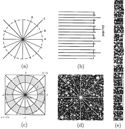
Note that rotation component w is perpendicular to translation component t for each pixel (x,y), and that w is inclependent of clepth. From this observa tion, rectification is performed on image seciuences to obtain optical snow motion (0,w2) + c(t2,0).
5.3.1 Motion Field Rectification
The rectification is a polar transformation around the FOE [651 which is the image center in our case. First, we rectify the motion field induceci by pure w
rotation. Consider a point p located in the image at (1,0) on the camera projection plane (see Fig. 5.2-a). The path followed through time hy p for a pure w2 movement is a circle of radius 1, and its speecl is exactly equal to w. The rectification is done by “unfolding” images such that this circle hecomes straight and vertical, as shown
35
FIG. 5.2 — (a) Original motion field (h) Rectified motion field (c) Rectified region
of the original sequence (cl) Original frame (e) Rectifieci frame
in Fig. 5.2-b. For a field of view of 900 alld images of size N x N, the vertical length of the rectified image is 2ir = irN pixels. Note that ftow unes of a pure forward
motion become horizontal. The velocities in the rectified motioi field correspond
fO ( ! f’T_(— -fzP/2..j..i P9’2w’Tzj
Standard optical snow produces velocities that only clepend on depth. However, the velocities in rectified nou-lateral motion sequences vary according to depth and to image position. Therefore, horizontal lines in the rectified sequence must be resampled according to factor /212 where (px’py) is the positio1 of a pixel on
py
the camera projection plane in the original sequeilce. In theory, we get infinite sampling at center (0,0). In practice, we do not rectify near the image ceuter as illustrated in Fig. 5.2-c. Notice that image corners are eut to remove empty spaces in the rectified sequence.
D
//
D C s A%I//IJ
(a) (b) (e) (e) (d)36 5.3.2 Finding rotation w,
The bowtie axis can 5e computed from the rectffied sequence using Principal Components Analysis as described in [63j• For standard optical
snow, the angle in the bowtie axis equation (see Proposition 2) is unknown. For non-lateral optical slow. however, we know that 900. Hence, the bowtie axis equation becomes (0, 1,w). Thus, the third component of the howtie axis gives us w clirectly with speed given in pixels/frame in the rectified sequence. The rotation giveil in degrees, for a field of view of 90° is then 360--.7rN
The bowtie axis can also 5e found using the best fit plane [63j
Let (nt, n, n,) 5e the normal of the best fit plane r. Since t is the only component affected hy depth, the bowtie axis is the une on the hest fit plane in direction (0, 1,
—p).
5.3.3 Finding translation t
From Eq. 5.5, and since t2 generates only horizontal velocities and w only vertical velocities, planes forming the howtie have equation (ot,,w,, 1). The best fit plane rr is defined as (, , 1) (t2,w2, 1), where is the weighted “average” of the slopes of the motion planes that compose the bowtie. The weights depend on depth distribution in the scene as well as image contrast contributed by each object. $ince this information is unknown, we can only compute t. up to a scale factor .
5.4 Experimental resuits
To evaluate our method, we rendered several synthetic image sequences of scenes containing lambertian spheres (see Fig. 5.3-a). Image motion was generated by moving a camera (90° field of view) through the scene with various t and w
parameters.
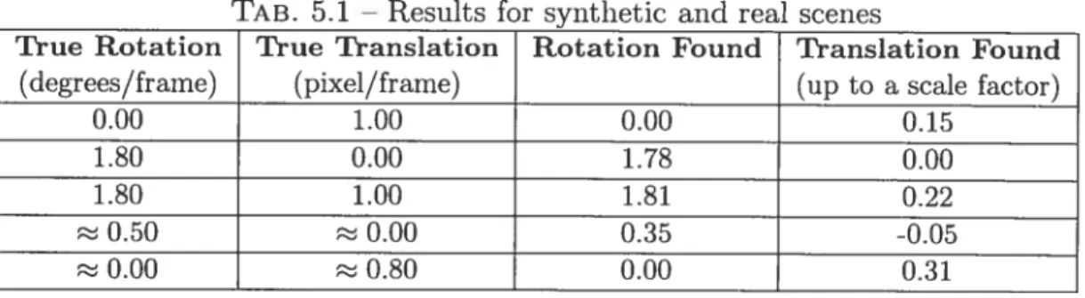
Table 5.1 shows results for various rectified sequences. The last two rows corres pond to real image sequences, respectively the laS sequence (see Fig. 5.3-b) and the plants sequence (see fig. 5.3-c). The w component is found almost exactly. The
37
FIG. 5.3 — (a) Svnthetic scenes were constitutecl of small bails at different depths
(64 frames of size 128x128 pixels). (b) Lab sequence taken from a camera rotating arounci the z-axis (40 frames of 128x128 pixels). (c) Pla;its sequence taken from a camera making a forward motion (32 frames of 128x128 pixels).
rmrning time is about 1.6 seconds for 128x128x32 sequences 011 a 1.3GHz AIVID Athion machine.
TAB. 5J Resuits for synthetic and real scenes
True Rotation True Translation Rotation Found Translation Found
(
degrees/frarne) (pixel/frame) (up to a scale factor)0.00 1.00 0.00 0.15
1.80 0.00 1.78 0.00
1.80 1.00 1.81 0.22
0.50 0.00 0.35 -0.05
0.00 0.80 0.00 0.31
5.5 Comparing the eigenvalues
When analyzing image sequences globally, we would like to estimate how well the motion fits the optical snow model, i.e. if a bowtie is present. For instance, an unrectifed forward motion or a rectified lateral motion do not produce a bow tie signature. For such cases, the motion fieid features velocities oriented in ail directions. Detecting these situations would be a great benefit.
jj [63] depth range is evaluated by comparing the two largest eigenvalues of
the Principal Components Analysis method. We can aclapt this measure to detect the presence of a bowtie. The ratio of the first two eigenvalues À2 and À1 lias a
38 maximum of 1 and should decrease as we get doser to a bowtie signature. In fact, the presence of a bowtie creates a high power concentration along its axis which increases the first eigenvahie. The absence of a bowtie is caracterized by a iiiform power distribution which makes ) and almost equal. Fig. 3.4-a shows a plot of as a fiinction of for rectified sequences. As expected, the ratio falis off as the bowtie takes shape in the frequency clomain. Fig. 3.4-b shows as a function of for non-rectified sequelwes. As expectecl, it increases linearl up to 1 as howtie signature clïsappears. The sequeices useci for these graphs have random translation vectors of unit length.
Notice that the curve in Fig. 3.4-a decreases noi-linear1y while the other one is linear. This might be caused by the subsampling during rectification which ac centuates the effect of aiy lateral motion. This is stiil imder investigation. These curves, if rnodelled correctly, would allow merging non-lateral and lateral motions analysis into a general egomotion estimation algorithm.
(a)
FIG. 5.4 — (a) as a ftmction of for rectified secluences. It starts rut 1 anci
decreases as a bowtie signature takes shape. (b) -- as a function of for no;
rectified sequences. It increases linearly up to 1 as bowtie signature disappears.
5.6 Conclusion
This paper presented a method to analyze purely non-lateral optical snow by introducing a rectification process. Results show its accuracy alld efficiency. We hope to solve the general egomotion problem in a global approach using this scheme.
• ,•.:. •: •. • .? • 0.75 • 0.7 0 65 (b)
CHAPITRE 6
DISCUSSION
Une nouvelle méthode PCA d’analyse du modèle de neige optique est présentée au chapitre 3 (voir le code à l’annexe II). Cette méthode trouve une ligne d’énergie dans la tranformée de Fourier 3D de la séquence. De plus, une rectification de la séquence vidéo, introduite au chapitre 5, permet l’estimation du mouvement de caméra vers l’avant (t2) et de la rotation par rapport à l’axe optique (w2). Par contre, les analyses de la séquence rectifiée et non rectifiée sont interdépendantes. Un modèle robuste permettant de mesurer la contribution des composantes ciblées dans la séquence originale (t,t,,w, w0) et celles ciblées dans la séquence rectifiée
(t2,w2) reste à établir. Plusieurs autres observations sont aussi nécessaires, dont certaines peuvent servir de pistes de recherche.
6.1 Algorithme biologiquement plausible pour l’analyse de la neige op tique
L’algorithme PCA recherche en fait une ligne dans le domaine fréquenciel. Plu sieurs méthodes ont déjà été proposées pour trouver de façon biologiquement plau sible un plan dans le domaine fréquentiel à l’aide de filtres de Gabor [50—52]
Il serait intéressant d’adapter ces algorithmes pour trouver non pas un plan, mais une ligne.
6.2 Distribution d’énergie uniforme
La méthode du prisme à base triangulaire de Langer et Mann [9] et la méthode PCA présentée au chapitre 3 sont complémentaires, en ce sens que la première mesure l’absence d’énergie et la deuxième, la présence d’énergie. Cette observation peut laisser croire que la méthode du prisme est pins robuste pour des scènes où les objets et le contraste dans l’image sont non uniformes.