INTER-NOISE 2006
3-6 DECEMBER 2006 HONOLULU, HAWAII, USA
Sound field modeling in architectural acoustics
using a diffusion equation
Judicaël Picauta LCPC, Centre de Nantes Route de Bouaye, BP 4129 44341 Bouguenais Cedex France Vincent Valeaub
LEA, Université de Poitiers 22 Avenue du Recteur Pineau
86022 Poitiers Cedex France
Alexis Billonc
LEPTAB, Université de La Rochelle Avenue Michel Crépeau 17042 La Rochelle Cedex 01
France
Anas Sakoutd
LEPTAB, Université de La Rochelle Avenue Michel Crépeau 17042 La Rochelle Cedex 01
France
ABSTRACT
A numerical approach is proposed to model the reverberated sound field in rooms. The model is based on the numerical implementation of a diffusion model enabling spatial variations of the sound energy within a room, unlike the statistical theory. The proposed method allows to take into account most of complex phenomena encountered in room acoustics, like mixed reflections on walls (diffuse and specular), low and high absorption on walls, atmospheric attenuation, fitted zones. Moreover, the model can be applied to complex geometries, like multiple coupled rooms of different sizes. In this paper, the model and its numerical implementation are first detailed. Then, an application is proposed for a complex geometry defined by multiple coupled rooms with fitting objects, including low and high absorption on walls, in terms of sound level and reverberation times. The main interest of the model is that such approach requires less computational time in comparison with common approaches like ray-tracing simulations.
1 INTRODUCTION
Coupled volumes and fitted rooms have attracted considerable attentions in architectural acoustics. Such configurations can be found in various buildings such as concert halls fitted with reverberation chambers, industrial halls or office spaces. In workspaces the user's acoustical comfort is of particular interest. In concert halls, a very high acoustic quality is required. The prediction of the different acoustical parameters (sound pressure levels, reverberation times, speech intelligibility, etc.) is then needed.
For coupled geometries, several models have been proposed such as statistical theory [1-3], statistical energy analysis [4], modal theory [5], finite-element methods [6] and ray-based models [7-9]. Despite being based on the diffuse-sound-field theory assumption, the statistical theory has been compared satisfactory with and numerical results. Nevertheless, different authors question the ability of the statistical theory to deal with room modes, geometric and acoustic details, as well as non-diffuse sound field [10]. The modal theory and the finite-elements methods are limited to the low-frequency range, due to increasing computation times at higher frequencies. The ray-based model have shown quite good agreements with experimental data, as well as with
a Email address: [email protected] b Email address: [email protected] c Email address: [email protected]
statistical models, provided that a large number of rays is emitted for small coupling apertures, which implies long computation times.
Various prediction models have also been proposed to describe the acoustics of fitted rooms. These include analytical models [11-13], empirical models [14] and simplified models [15]. Numerical models have also been developed, based on the ray-tracing concept. Although they achieve reasonable agreement with measurement data [16,17], most of them have limited applicability, and cannot be mixed with models for coupled rooms.
This quick review shows that a model allowing spatial variations of the reverberant sound field in coupled and fitted rooms, both in terms of sound level and sound decay, with acceptable computation times, is needed.
In recent papers [18-20], a generalization and a numerical implementation of a diffusion model [21-22], for coupled geometries and fitted rooms. The model has been validated both in stationary and time-varying states. The main interest of the model is its ability to give satisfactory results in only a few seconds or minutes. Moreover the sound decay and the sound level can be calculated at any location in the coupled or fitted volume.
In this paper, an application of the diffusion model is proposed for a complicated configuration composed of an industrial hall with fitting objects coupled with offices to show the interest of the model. At first, the diffusion model is described in the next section.
2 DIFFUSION MODEL
2.1 Theory
In recent papers [21-22], a diffusion model was proposed to simulate the sound fields in rooms with diffusively reflecting boundaries. It was shown that the energy flow per unit surface J(r,t) in a direction n and at location r in the room, may be described by a diffusion gradient equation: ) , ( gradw t Dr r J= − , (1)
where w(r,t) is the acoustic energy density and Dr is a diffusion coefficient which can be written
as Dr =λrc/3, c being the sound velocity and λr the mean free path of the room (equal to 4V=S, V
being the room volume and S the total area of the surfaces of the room). The energy density in the room, outside the direct field, is then described by a diffusion equation [18]:
) , ( ) , ( ) , ( ) , ( mcw t F t t t w t w Dr r r − r = r ∂ ∂ − ∆ , (2)
where F(r,t) is the acoustic source term and m the coefficient of atmospheric absorption. The absorption of acoustic energy at boundaries is taken into account by an exchange coefficient h. For a boundary with low absorption coefficient αr , it can be shown [22] that the energy flow J
through the surface verifies:
) , ( ) , ( ) , ( t Dr w t hwr t n r n r J = ∂ ∂ − = ⋅ , (3)
with h=cαr /4 is defined as an exchange coefficient. For larger absorption, the Sabine's absorption
coefficient αr can be replaced by the Eyring's absorption coefficient -ln(1-αr ).
For simulating the acoustics of coupled rooms connected by open apertures [19], the system of equations (2) and (3) is solved in each room by setting the diffusion coefficient, then the mean free path, to the value that it would have if the rooms were uncoupled. That means that the coupling aperture area is small compared to the area of the wall surfaces for each room, so that the mean free path is not much affected by the open aperture.
A sub-volume Vf of V may also contains scatterers, statistically defined by their density nf
(i.e. the number of scattering objects per unit volume), their average scattering cross-section Qf
and their absorption coefficientαf. The diffusion by scatterers is then characterized by the mean
free path λf=1/nf Qf . The diffusion equation (2) is then replaced by (see Ref. [20])
) , ( 4 ) , ( ) , ( ) , ( mcw t c F t t t w t w D r r − r + f = r ∂ ∂ − ∆ α , (4)
where the new diffusion coefficient D=λc/3 is defined by considering the sound diffusion both by the room and the scatterers, such as the mean free path λ is now given by:
f r f r λ λ λ λ λ + = . (5) 2.2 Numerical implementation
The numerical method used for solving the diffusion equation (2) and/or (4) together with the boundary conditions (3) is based on the finite-element method (FEM) [18]. Let us mention here that the most important limitation of finite element methods (i.e. the size of the elements) is not strictly a problem with this model, since the size of the elements is more dependent on the mean free path than on the wavelength, as it is usually encountered to solve the Helmholtz equation. Moreover, the same meshing can be applied for all frequency bands, since the frequency is only taken into account in the absorption coefficients of the room boundaries. However, the size of the element should be on the order (or smaller) of one mean free path. Thus, the diffusion model can be applied to very large enclosures with a limited meshing.
3 APPLICATION
3.1 Geometry
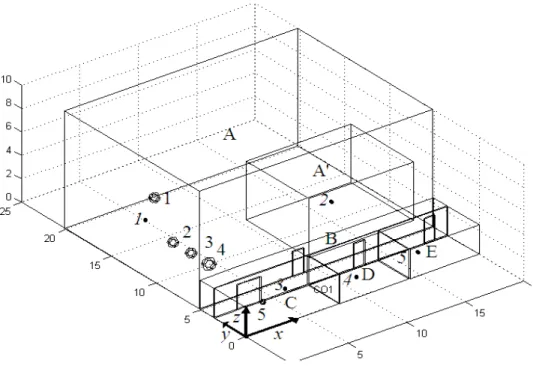
To exhibit the interest of the diffusion model, a configuration, similar to a small factory, with a rather complicated geometry is presented in Figure 1. It is made up of a hall A (20x25x10 m3) ,
a corridor B (20x2.5x2.5 m3) and three rooms C, D and E.
Four sound sources with different sound power level are located in the hall A: source 1 (120 dB) and sources 2, 3 and 4 (100 dB). The walls of the hall are in concrete (α=0.03). A fitting zone, defined by fitting objects with absorption α=0.3 and density nf=0.25 m, is localized in a
volume A’ (9x7x5 m3) of the hall A.
The hall A is connected through a 0.9x2.1 m² aperture to the corridor B. In this study, two cases are considered: a specularly reflecting corridor with a homogeneous absorption α=0.06 and a treated one, fully diffuse, and with an absorbent ceiling (α=0.6).
Rooms D and E are offices (5.9x3.5x2.5 m3) with homogeneous absorption (α=0.06) and are
connected to the corridor B through apertures of size 0.9x2.1 m². The room C is a small workshop (α=0.03) containing a sound source (source 5) with a sound power 100dB, and is connected to the corridor B through a aperture of size 2x2.1 m².
The atmospheric sound attenuation is set to 0.005 dB/m. The italic numbers on Figure 1 show the position where the sound decays are estimated.
The geometry is discretized in more than 110 000 Lagrange linear type elements. The diffusion equation is solved using a finite elements solver (FEM). Computation time is around 30 s for the steady state sound level and 5 min for the time-varying problem (5 receivers) calculated along 1.5 s with 0.02 s time steps.
Figure 1: Geometry of the studied configuration: hall A, corridor B, workshop C, offices D and E. Sound sources (1 to 5) and receivers locations (1 to 5, with italic numbers) are also given.
A fitting zone A' , containing the receiver 2, is also considered in the hall A.
3.2 Steady-state results
As presented on the previous section, the diffusion model allows to give the sound pressure level SPL at any location in the studied configuration, whatever the complexity of the geometry. As example, a slice of the SPL of the reverberated sound field at 1.2 m high, in the enclosure, is presented in Figure 2.
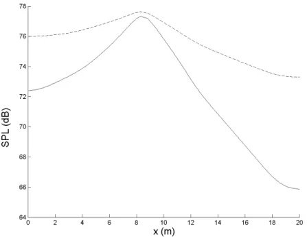
In particular, one can observed the decrease of SPL in the fitting zone, in comparison with the SPL in the hall, due to larger absorption of the fitting objects in comparison with the wall absorption.
The effect of the corridor treatment is also clearly showed in the connected rooms, with a decrease of the SPL in room E of about 5 dB, for example. The effect of treatment is more clearly exhibited in Figure 3 which plots the SPL along the corridor at 1.2 m high, with and without treatment. The increase of acoustics absorption and the effect of diffuse reflections in the
corridor raise the sound attenuation of more than 8 dB. The acoustics treatment in the corridor is also responsible for the decrease of the sound energy within the offices (D and E).
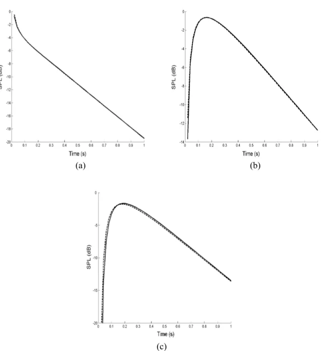
3.3 Sound decay results
Sound decays at the locations 1, 3 and 5 are presented in Figure 4. This figure shows that the influence of the corridor treatment is very weak on the reverberation times, since the sound decay are similar with and without the treatment.
(a) non treated configuration
(b) treated configuration
Figure 2: Sound pressure level of the reverberant sound at 1.2 m for the non treated configuration (a), and for the treated configuration (b).
Figure 3: SPL along the corridor at 1.2 m high: (- -) non treated corridor, () treated corridor.
In the hall (Figure 4(a)), a double sloped decay can be observed: the first one is due to the spreading of the acoustical energy throughout the building and the second one is produced by the reverberant sound field in the hall. The other two decays are similar (Figure 4(b) and Figure 4(c)).
4 CONCLUSIONS
The main interest of this approach, is its ability to give satisfactory results whatever the room shapes, at any receiver locations, in few seconds only for a stationary state, and in few minutes for a time-varying state, while most of current softwares need extensive computational time.
Although, this is not given in this paper, the diffusion model have also been compared to experimental data and numerical model, like ray-tracing, with a good agreement, both for coupled rooms and rooms with fitting objects [18-20].
Moreover, the most important limitation of finite element methods (i.e. the size of the elements) is not strictly a problem in this case, since the size is more dependent on the mean free path than on the acoustic wavelength. Thus, the diffusion model can be applied to very large enclosures with a limited meshing.
Such approach could be used in a first step of an architectural project, to calculate and to design the main acoustical features of a room (sound field distribution and decay), while a classical approach, like ray-tracing software, could be used in a second step, to give more specific and accurate results.
(a) (b)
(c)
Figure 4: Normalized sound decays at locations 1 (a), 3 (b) and 5 (c): (- -) non treated corridor, () treated corridor.
5 REFERENCES
[1] C. F. Eyring, “Reverberation time measurements in coupled rooms,” Journal of the Acoustical Society of America, 3(2), 181–206 (1931).
[2] L. Cremer and H. Muller, Principles and applications of room acoustics, volume 1 (Applied Science Publishers, London, 1978).
[3] J. E. Summers, R. R. Torres, and Y. Shimizu, “Statistical-acoustics models of energy decay in system of coupled rooms and their relation to geometrical acoustics,” Journal of the Acoustical Society of America, 116(2), 958–969 (2005).
[4] C. B. Burroughs, R. W. Fischer, and F. R. Kern, “An introduction to statistical energy analysis,” Journal of the Acoustical Society of America, 101(4), 1779–1789 (1997).
[5] C. Thompson, “On the acoustics of a coupled space,” Journal of the Acoustical Society of America, 75(3), 707–714 (1984).
[6] Y. Zhao and S. Wu, “Acoustical normal mode analysis for coupled rooms,” Proceedings of the 21st International Conference of the Audio Engineering Society (2002).
[7] J. E. Summers, R. R. Torres, Y. Shimizu, and B.-I. L. Dalenbäck, “Adapting a randomized beam-axis-tracing algorithm to modeling of coupled rooms via late-part ray tracing,” Journal of the Acoustical Society of America, 118(3), 1491–1502 (2005).
[8] M. Ermann, “Coupled volumes: Aperture size and the double sloped decay of concert halls,” Building Acoustics 12(1), 1–14 (2005).
[9] D. T. Bradley and L. M. Wang, “The effects of simple coupled volume geometry on the objective and subjective results from non exponential decay,” Journal of the Acoustical Society of America, 118(3), 1480–1490 (2005).
[10]J. E. Summers, “Comments on ‘absorbing surfaces in ray-tracing programs for coupled spaces’,” Applied Acoustics, 64, 825–831 (2003).
[11]E. A. Lindqvist, “Sound attenuation in large factory spaces,” Acustica, 50(5), 313–328, (1982).
[12]U. J. Kurze, “Scattering of sound in industrial spaces,” Journal of Sound and Vibration, 98(3), 349–364 (1985).
[13]M. Hodgson, Physical and theoretical models as tools for the study of factory sound fields, PhD Dissertation (University of Southampton, 1983).
[14]N. Heerema and M. Hodgson, “Empirical models for predicting noise levels, reverberation times and fitting densities in industrial workrooms,” Applied Acoustics, 57, 51–60 (1999). [15]A. M. Ondet and J. L. Barbry, “Modeling the sound propagation in fitted workshops using
ray tracing,” Journal of the Acoustical Society of America, 85, 787–796 (1989).
[16]M. Hodgson, “Experimental evaluation of simplified models for predicting noise levels in industrial workrooms,” Journal of the Acoustical Society of America, 103(4), 1933–1939 (1997).
[17]M. Hodgson, “Ray-tracing evaluation of empirical models for predicting noise in industrial workshops,” Applied Acoustics, 64, 1033–1048 (2003).
[18]V. Valeau, J. Picaut, and M. Hodgson, “On the use of a diffusion equation for room acoustic predictions,” Journal of the Acoustical Society of America 119(3), 1504–1513 (2006).
[19]A. Billon, V. Valeau, J. Picaut, and A. Sakout, “On the use of a diffusion model for coupled rooms,” Journal of the Acoustical Society of America (in press).
[20]V. Valeau, J. Picaut, and M. Hodgson, “A diffusion-based analogy for the prediction of sound fields in fitted rooms,” Acta Acustica united with Acustica (in press).
[21]J. Picaut, L. Simon, and J.-D. Polack, “Sound field in long rooms with diffusely reflecting boundaries,” Applied Acoustics, 56, 217–240 (1999).
[22]J. Picaut, J. Hardy, and L. Simon, “Sound field modeling in streets with a diffusion equation,” Journal of the Acoustical Society of America, 106, 2638-2645 (1999).