Sensitivity analysis of oscillator models in the space of phase response curves: Oscillators as open systems

Digital Object Identifier 10.1109/MCS.2013.2295710

O

scillator models—whose steady-state behavior is periodic rath-er than constant—are fundamental to rhythmic modeling, and they appear in many areas of engineering, physics, chemistry, and biology [1]–[6]. Many oscillators are, by nature, open dy-namical systems in that they interact with their environment [7]. Whether functioning as clocks, information transmitters, or rhythm generators, these oscillators have the robust ability to respond to a par-ticular input (entrainment) and to behave collectively in a network (syn-chronization or clustering).

Date of publication: 14 March 2014

OscillatOrs as Open systems

Pierre SacrÉ and

rodolPhe SePulchre

Sensitivity Analysis

of Oscillator Models

in the Space of

The phase-response curve of an oscillator has emerged as a fundamental input–output characteristic of oscillators [1]. Analogously to the static (zero-frequency) gain of a transfer function, the phase-response curve measures a steady-state (asymptotic) property of the system output in response to an impulse input. For the zero-frequency gain, the measured quantity is the integral of the response; for the phase-response curve, the measured quantity is the phase shift between the perturbed and unperturbed responses. Because of the periodic nature of the steady-state behavior, the magnitude and the sign (advance or delay) of this phase shift depend on the phase of the impulse input. The phase-response curve is therefore a curve rather than a scalar. In many situations, the phase-response curve can be determined experimentally and pro-vides unique data for the systems analysis of the oscillator. Alternatively, numerical methods exist to compute the phase-response curve from a mathematical model of the oscillator. The phase-response curve is the fundamental mathematical information required to reduce an n-dimen-sional state-space model to a one-dimenn-dimen-sional (phase) center manifold of a hyperbolic periodic orbit.

Motivated by the prevalence of the input–output repre-sentation in experiments and the growing interest in sys-tem-theoretic questions related to oscillators, this article extends fundamental concepts of systems theory to the space of phase-response curves. Comparing systems with a proper metric has been central to systems theory (see [8]– [11] for exemplative milestones). In a similar spirit, this article aims to endow the space of phase-response curves with the right metrics (accounting for natural equivalence properties) and sensitivity analysis tools. This framework provides mathematical and numerical grounds for robust-ness analysis and system identification of oscillator models. Although classical in their definitions, several of these tools appear to be novel, particularly in the context of bio-logical applications.

The focus of the article is on oscillator models in sys-tems biology and neurodynamics—two areas where sensi-tivity analysis is particularly useful to assist the increasing focus on quantitative models. In systems biology, phase-response curves have been primarily studied in the context of circadian rhythms models [4], [12], [13]. A circadian oscilla-tor is at the core of most living organisms that need to adapt their physiological activity to the 24-h environmental cycle associated with the earth’s rotation (for example variations

in light or temperature condition). Circadian oscillators have a period close to 24 h under constant environmental conditions and can lock oscillations (in frequency and phase) to an environmental cue that has a period equal to 24 h. In neurodynamics, the use of phase-response curves is more recent but increasingly popular [14]. A spiking oscil-lator is the repeated discharge of action potentials by a neuron, which is the basis for neural coding and informa-tion transfer in the brain. This oscillatory system is capable of exhibiting oscillations on a wide range of periods—from 0.001 to 10 s—and of behaving collectively in a neural net-work. Phase-response curves are also used in many other areas of sciences and engineering (such as planar particle kinematics, Josephson junctions, and alternating current power networks) for which the reader is referred to the abundant literature (see, for example, the pioneering con-tributions [1], [2], [15]–[18], and the detailed review [19, and references therein]).

The results of the article are primarily drawn from the Ph.D. dissertation of the first author [20]. A preliminary version of this work was presented in [21]. The first case study on circadian rhythms was discussed in detail in [22].

The article is organized as follows. The first section presents the concept of phase-response curves derived from phase-resetting experiments. The second section is a review of the notion of phase-response curves character-izing the input–output behavior of an oscillator model in the neighborhood of an exponentially stable periodic orbit. The third section defines several relevant metrics on (nonlinear) spaces of phase-response curves induced by natural equivalence properties. The fourth section devel-ops the sensitivity analysis for oscillators in terms of the sensitivity of its periodic orbit and its phase-response curve. The fifth section illustrates how these tools solve system-theoretic problems arising in biological systems, including robustness analysis, system identification, and model classification.

The main developments of the article are supple-mented by several supporting discussions. “A Brief His-tory of Phase-Response Curves” sets the use of phase-response curves in its historical context. “Phase Maps” defines the key ingredients for studying oscillator models on the unit circle. “From Infinitesimal to Finite Phase-Response Curves” provides details on the mathe-matical relationship between finite and infinitesimal phase-response curves. “Basic Concepts of Differential

The article describes a framework for the analysis of oscillator

models in the space of phase-response curves and to answer

Geometry on Manifolds” and “Basics Concepts of Local Sensitivity Analysis” present distinct features of differ-ential geometry and sensitivity analysis used in this article, respectively. “Numerical Tools” provides the numerical tools to turn the abstract developments into concrete algorithms. The notation is defined in “List of Symbols.”

PhASE-RESPONSE CuRvES fROM

ExPERIMENTAL DATA

The interest of a biologist in an oscillator model comes through the observation of a rhythm, that is, the regular repetition of a particular event. Examples include the onset of daily locomotor activity of rodents, the initiation of an action potential in neural or cardiac cells, or the onset of mitosis in cells growing in a tissue culture (see “A Brief History of Phase-Response Curves”). One of the simplest modeling experiments is to perturb the oscillatory behav-ior for a short (with respect to the oscillation period) dura-tion and record the altered timing of subsequent repeats of the observable event. Once the system has recovered its prior rhythmicity, the phase of the oscillator is said to have reset. In general, the phase reset depends not only on the perturbation itself (magnitude and shape) but also on its timing (or phase) during the cycle. This section formalizes the basic experimental paradigm of phase-resetting experi-ments and describes the concept of phase-response curves following the terminology in [1] and [3].

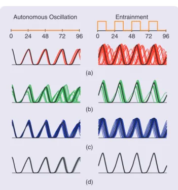
An isolated oscillator (closed system) exhibits a precise rhythm, that is, a periodic behavior, and the period T of the rhythm is assumed constant [see Figure 1(a)]. To facili-tate the comparison of rhythms with different periods (for example, due to the variability in experimental prep-aration), it is convenient to define the notion of phase. In the absence of perturbations, the phase is a normalized time evolving on the unit circle. Associating the onset of the observable event with phase 0 (or 2r), the phase

vari-able ( )i t at time t corresponds to the fraction of a period elapsed since the last occurrence of the observable event. It evolves linearly in time, that is, ( ) :i t =~(t t-

t

i)(mod2r), where :~=2r/T is the angular frequency of the oscillator and t

t

i is the time of the last observable event.

Following a phase-resetting stimulus at time (ts-

t

t0)after one observable event (open system), the next event times ,

t

ti for

,

i!N>0 are altered. For simplicity, it is assumed that the origi-nal rhythm is restored immediately after the first post-stimu-lus event, meaning that observable events repeat with the original period T [see Figure 1(b)]. The duration :T

t

=

t

t1-

t

t0 denotes the time interval from the event immediately before the stimulus to the next event after stimulation. Once again, it is convenient to normalize each quantity to facilitate compari-son between different experimental preparations. Multiplying by ~=2r/T leads to i:=~(ts-t

t

0) and x

t

:=~T

t

=~(

t

t1-

t

t0).

The effect of a stimulation is to produce a phase shift Di

between the perturbed oscillator and the unperturbed oscillator. The phase shift Di is

Input 0 0 0 0 Input Output T T T T T T T Output (b) (a) T^ t_s t^₁ t₀ ^ t_₁ ^ _t 2 ^ _t 3 ^

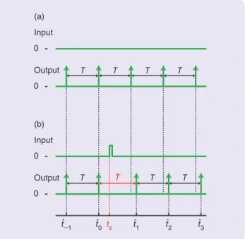
Figure 1 A schematic representation of a phase-resetting experi-ment. (a) In isolated conditions (closed system), the observable event (vertical arrow) occurs every T units of time. (b) Following a phase-resetting stimulus at time t^s- tt0h after an event (open

system), the successive observable event times ,tt for i i!N20, are

altered. :Tt =tt1-tt denotes the time interval between the pre- and 0

post-stimulus events.

List of Symbols

u Input value of a system

y Output value of a system

x State variable of a system c Periodic orbit of an oscillator

xc _{Zero-input steady-state solution of an oscillator}

H Asymptotic phase map of an oscillator i Phase variable of an oscillator

Q (Finite) phase-response curve

q Infinitesimal phase-response curve

p Gradient of the asymptotic phase map evaluated along the periodic orbit, ( ):p$ =dxH( ( ))\c $

R Set of real numbers

Rn n-dimensional Euclidean space

S1 Set of points on the unit circle, S1:=R/(2rZ) N Set of natural numbers

x

_o

Derivative, with respect to time, of the variable x

xl Derivative, with respect to phase, of the variable x

0 Input identically equal to zero

z* _{Complex conjugate of the complex number z}

AT _{Transpose of the matrix A}

( , )x y Equivalent notation for the vector [x yT T T]

x 3 Maximum norm of the vector x , x 3: max=

: 2 (wrap to [ , )),

i r x r r

D = -

t

-where the operation x (wrap to [-r r, ))=[x+r(mod2r)]

r

- wraps x to the interval [-r r, ) (see Figure 2). Given a

phase-resetting input ( ),u $ the dependence of the phase shift Di on the (old) phase i at which the stimulus was

delivered is commonly called the phase-response curve. It is denoted by ( ; ( )),Qi u$ to stress that it is a function of the phase but that it also depends on the input ( )u $.

An alternative representation emphasizes the new phase i+ instead of the phase difference. Just before the

stimulus, the oscillator had reached old phase ;i just after,

the oscillator appears to resume from the new phase : 2 ( ) (mod2 ).

i+= r-x

_t

-i r

Given a phase-resetting input ( ),u $ the dependence of the new phase i+ on the (old) phase i at which the stimulus

was delivered is called the phase-transition curve denoted by ( ; ( )).u

Ri $

Under the approximation that the initial rhythm is recovered immediately after the perturbation, the phase shift computed from the first post-stimulus event is identi-cal to the asymptotic phase shift computed long after the perturbation. This assumption neglects the transient change in the rhythm until a new steady state is reached. To model the transient, the normalized time from the event before the stimulus to the ith event is denoted by

: (t t),

i i 0

x

t

=~

t t

- leading to the phase shift D =ii: 2r -(wrap to [ , ))

i

x

t

-r r and the new phase i+i :=2r-(x

_t

i-i)

(mod 2r). If the oscillating phenomenon is time invariant,

a new steady-state behavior is expected asymptotically, such that limi"3(x

t

i+1-x

t

i)=2r, limi"3Dii=:Di, and

: limi"3ii+=i+.

PhASE-RESPONSE CuRvES fROM

STATE-SPACE MODELS

This section reviews the mathematical characterization of phase-response curves for oscillators described by time-invariant, state-space models.

State-Space Models of Oscillators

Limit cycle oscillations appear in the context of nonlinear time-invariant, state-space models

( , ), xo =f x u (1a) ( ), y=h x (1b) 0 (wrap to [-r, r)) x x 0 0 3r -3r S1 -r r r

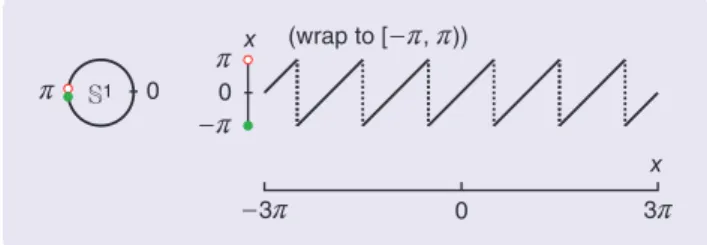
Figure 2 A graphical representation of the wrap-to-[-r r, ) oper-ation. Given a real number x in radians, x (wrap to [-r r, ))/ [x+r(mod2r)]-r wraps x to the interval [-r r, ). It adds or subtracts an integer multiple of 2r such that the result belongs to [-r r, ). (A solid dot indicates that the end point is included in the set, whereas an open dot indicates that the end point is excluded from the set.)

A Brief History of Phase-Response Curves

P

hase-response curves were used for the first time in 1960

by a biological experimentalist to represent the results of phase-resetting experiments on the rhythm of the daily loco-motor activity in flying squirrels [12]. The author was inves-tigating the effect of short light pulses on the daily onsets of running activity in the wheel in constant darkness. The response to these stimulations varied according to the time of the day—the squirrel’s subjective day—at which the light pulse was administered. To represent her data, the author plotted the observed time shift (advance or delay) as a func-tion of time of perturbafunc-tion.

PhASE-RESPONSE CuRvES IN BIOLOGY

Phase-response curves are widely used to study biological rhythms (see the pioneering book [1]). The two main applications are circadian rhythms and neural (or cardiac) excitable cells.

In circadian rhythms, the phase-response curve is used to study the effect of light (and sometimes the effect of drugs, such as melatonin) on the rhythm. In particular, the mecha-nism of entrainment to light is of critical importance in

circa-dian rhythm studies. Numerous experimental phase-response curves for circadian rhythms have been compiled in an atlas [74]. Most of these phase-response curves have a typical shape including a dead zone, which is an interval of zero sen-sitivity during the subjective day of the studied organism.

In neural (or cardiac) excitable cells, the phase-response curve is used to study ensemble behavior in a network, par-ticularly, synchronization in coupled neurons and entrainment in uncoupled neurons subject to correlated inputs (also known as stochastic synchronization). The book [14] compiles several applications of phase-response curves in neuroscience.

PhASE-RESPONSE CuRvES IN ENGINEERING

Phase-response curves are not often used in engineering applications. An exception is in electronic circuits, where the concept of a perturbation projection vector was developed to study phase noise in oscillators [75]–[79]. Mathematically, the perturbation projection vector is identical to the infinitesimal phase-response curve. It is used as a reduction tool to study oscillators and to design electronic circuits [80].

where the states ( )x t evolve on some subset X3Rn, and the input and output values ( )u t and ( )y t belong to subsets U3R and Y3R, respectively. The vector field

:

f X#U"Rn and the measurement map :h X"Y support all the usual smoothness conditions necessary for the exis-tence and uniqueness of solutions. An input is a signal

: [ , )

u 03 "U that is locally essentially compact (meaning that images of restrictions to finite intervals are compact). The solu-tion at time t to the initial value problem x

o

=f x u( , ) from the initial condition x0!X at time zero is denoted by ( , , ( ))z t x u0 $ [with ( , , ( ))z 0x u0 $ =x0]. For convenience, single-input and single-output systems are considered. All developments gen-eralize to multiple-input and multiple-output systems.

The state-space model (1) is called an oscillator if the zero-input system x

o

=f x( , )0 admits an exponentially stable limit cycle, that is, a periodic orbit c3X with period T that attracts nearby solutions at an exponential rate [23]. Picking an initial condition x0c!c, the periodic orbit c is described by the locus of the (nonconstant) T -periodic solution ( , , ),z $ x0c0 that is,

: x!X:x ( , , ),t x0 0 t![ , ) ,0T

c=" =z c ,

where the period T> 0 is the smallest positive constant such that ( , , )z t xc0 0 =z(t T+ , , )xc0 0 for all t$0 and 0 is the

input signal identically equal to zero for all times. The peri-odic orbit is an invariant set.

Because of the periodic nature of the steady-state behav-ior, it is appealing to study the oscillator dynamics directly on the unit circle .S1 The key ingredient of this phase reduction is the phase map concept. A phase map : ( )H B c 3

S

X" 1 is a mapping that associates with every point in the basin of attraction ( )Bc 3X a phase on the unit circle .S1 Away from a finite number of isolated points (called singu-lar points), the phase map H is a continuous map. The phase variable ( )i t is the image of the flow through the phase map, that is, ( ) :i t =H( ( , , ( ))).z t x u0 $ By the definition of the phase map, the phase dynamics reduce to i

o

=~ for

the input 0. For nonzero inputs, the phase dynamics are often hard to derive. See “Phase Maps” for details.

For convenience, the periodic orbit c is parameterized by

the map :x S1_"

c

c _{that associates with each phase}

i on the

unit circle a point ( / , , )z i ~x0c0 =:xc( )i on the periodic orbit.

Response to Phase-Resetting Inputs

If a solution of (1) asymptotically converges to the periodic orbit, the corresponding input ( )u $ is said to be phase reset-ting. If an input is phase resetting for an initial condition ,x0 then there exists a (reset) phase i+!S1 that satisfies

( , , ( )) ( , ( / , , ), )0 0 . lim t x u t x 0 t"3 z 0 $ -z z i ~ 0 2= c +

Definition 1

Given a phase-resetting input ( ),u $ the (finite) phase-response curve is the map ( ; ( )) :Q$ u $ S1"[-r r, ) that associates with each phase i a phase shift D =i Q( ; ( )),iu$ defined as

( ; ( )) ( ( , ( ), ( ))) ( ) (wrap to , )). lim Qiu $ _t z t x i u$ ~t i r r H = - + -" 3 c + 6 6 @ Similarly, the phase-transition curve is the map ( ; ( )) :R u$ $ S1"S1 that associates with each phase i the new phase

( ; ( )),u R $ i+= i _{defined as} ( ; ( )) lim ( ( , ( ), ( ))) (mod ). R u t x u t 2 t $ $ i = H z i -~ r " 3 c + 6 @

A mathematically more abstract—yet useful—tool is the infinitesimal phase-response curve. It captures the same information as the finite phase-response curve in the limit of Dirac delta input with infinitesimal amplitude (that is,

( ) ( )

u $ =a d $ with a"0).

Definition 2

The infinitesimal phase-response curve is the map :q S1"R, defined as the directional derivative

( ) : ( ( )) _uf ( ( ), )x , q i =D xH c i ;₂2 c i 0E where ( ) : lim ( ) ( ). D x x h_h x h 0 h h H = H + -H " 6 @

The directional derivative can be computed as the inner product in Rn ( ) ( ( )) ( ( ), ) ( ( )), ( ( ), ) , q D x _uf x x _uf x 0 0 x 2 2 d 2 2 i i i i i H H = = c c c c ; E (2) where dxH(xc( ))i =: p( )i _{is the gradient of the asymptotic}

phase map H at the point ( )xc i.

The main benefit of an infinitesimal characterization of phase-response curves is that the concept is independent of the input signal. Limitations of the infinitesimal approach have been well identified since the early days of phase-resetting studies [1] and strongly depend on the application context. For instance, infinitesimal phase-response curves have proven very useful in the study of circadian rhythms [24] but come with severe limitations in the context of neu-rodynamics, as recently studied in [25]–[27].

Remark

By definition, the finite phase-response curve for an impulse input is well approximated by the infinitesimal phase-response curve, that is, ( ;Q$ a d( ))$ =aq( )$ +O( ).a2 See “From

Infinitesimal to Finite Phase-Response Curves” for details.

Phase Models as Reduced Models of Oscillators

Phase-response curves are the basis for the reduction of n-dimensional state-space models of oscillators to one-dimensional phase models. Phase models are the main rep-resentation of oscillators for networks. However, the focus of this article is on single oscillator models. For a compre-hensive treatment of phase models, the reader is referred to

pioneering papers [15], [16], [28], and [29]; review articles [19], [30], and [31]; and books [1], [3], [6], [14], and [32].

Below is a review of two popular phase models obtained through phase reduction methods in the case of weak input and impulse train input, respectively.

Under the simplifying assumption of weak input, that is, | ( )|u t %1, for allt$0,

any solution ( , , ( ))z t x u0 $ of the oscillator model that starts in the neighborhood of the hyperbolic stable periodic orbit c stays in its neighborhood. The n-dimensional

state-space model (1) can thus be approximated by a one-dimensional continuous-time phase model (see [2], [6], [30], and [32]–[34])

( ) ,u q

io=~+ i (3a)

Phase Maps

P

hase maps, as well as the associated notion of isochrons, are key ingredients for studying oscillator models. The below exposition of phase maps follows the terminology and definitions of [1] and [3]. The notation is illustrated in Figure S1.

Consider an oscillator described by (1).

The basin of attraction of c (the oscillator stable set) is the maximal open set from which the periodic orbit c attracts, that is, ( ) : {x : lim dist( ( , , ), )t x 0 0}, B X t 0! 0 c = z c= "+3

where dist( , ) : infxc = y!c x y- 2 is the distance from the point

x!X to the set c3X based on the Euclidean norm $ 2

in Rn.

Since the periodic orbit c is a one-dimensional manifold in ,

Rn it is homeomorphic to the unit circle S1. It is thus naturally parameterized in terms of a single scalar phase. The smooth bijective phase map :Hc"S1 associates with each point x on the periodic orbit c its phase ( ) :Hx =j on the unit circle ,S1 such that

( / , , ) .

x-z j ~xoc0 =0

This mapping is constructed such that the image of the ref-erence point x0

c

is equal to zero (that is, ( )Hx0 =0

c

) and the progression along the periodic orbit (in absence of perturba-tions) produces a constant increase in .j The phase vari-able : Rj $0"S1 is defined along each zero-input trajectory

( , , )$ x00

z starting from a point x0 on the periodic orbit ,c as

( ) :t ( ( , , ))t x00

j =H z for all times t$0. The phase dynamics are thus given by j

o

=~.

For a hyperbolic stable periodic orbit, the notion of phase can be extended to any point x in the basin ( )B c by defining the concept of asymptotic phase. The asymptotic phase map

: ( )B c "S1

H associates with each point x in the basin ( )B c its asymptotic phase ( ) :H x =i on the unit circle ,S1 such that

( , , ) ( , ( / , , ), ) .

lim t x0 t x00 0 2 0

t z -z z i ~ =

c

"+3

Again, this mapping is constructed such that the image of x0c

is equal to zero and such that the progression along any orbit in B( )c (in absence of perturbations) produces a constant increase in .i The asymptotic phase variable : Ri $0"S1 is

defined along each zero-input trajectory z^$, ,x00h starting from

a point x0 in the basin of attraction of c as i^th:=H^z( , , )t x00h

for all times t$0. The asymptotic phase dynamics are thus given by i

o

=~.

The notion of the asymptotic phase variable can be extended to any nonzero-input trajectory ( , , ( ))z$ x u0 $ in the

basin of attraction of c. In this case, the asymptotic phase variable is defined as ( ) :i t =H( ( , , ( )))zt x u0 $ for all times t$0.

Thus, the phase variable ( ),it) at an instant t)$0, evaluates

the asymptotic phase of the point ( , , ( )).zt x u) 0 $ The asymptotic

phase dynamics in the case of a nonzero input are often hard to derive.

Level sets of the asymptotic phase map ,H that is, sets of all points in the basin of c with the same asymptotic phase, are termed isochrons. Formally, the isochron ( )Ii associated with the asymptotic phase i is the set ( ) :Ii ="x!B( ): ( )c H x =i,. Considering hyperbolic periodic orbits, isochrons are codi-mension-1 submanifolds (diffeomorphic to Rn 1- _{) crossing the}

periodic orbit transversally and foliating the entire basin of attraction [81].

In general, the (asymptotic) phase maps and their isochrons are complex, which often makes analytical computation impos-sible and even numerical computation intractable (or at least expensive, particularly for high-dimensional oscillator models). Most numerical techniques rely on backward integration [82]– [84]. An elegant forward integration method was developed in [85] and extended to stable fixed points in [86].

H : B(c) " S1 0 i S1 x I(i) x₀c B(c)

Figure s1 An asymptotic phase map and isochrons. The asymp-totic phase map :HB^ hc "S1 associates with each point x in the basin of attraction B^ hc a scalar phase H^ hx =i on the unit circle S1 such that limt" 3 zt x, ,0 -zt+i ~/ , ,x00 2=0.

c

+ ^ h ^ h The image

of x0c through the phase map H is equal to zero. The set of points

associated with the same phase i (that is, a level set of the phase map) is called an isochron and is denoted by I^ hi .

( ),

y= uhi (3b)

where the phase variable i evolves on the unit circle .S1 The phase model is fully characterized by the angular fre-quency ~> 0, the infinitesimal phase-response curve

: ,

q S1"R and the measurement map :_{h S}

u

1"Y, which is defined as ( )h

u

i =h x( ( )).c i

An alternative simplification is when the input is a train of resetting impulses, that is,

( ) ( ), with , u t t t t 0 k k k 0 $ a d = -3 =

/

where it is assumed that the time interval between succes-sive impulses is sufficient for convergence to the periodic orbit between each of them. Under this assumption, any solution ( , , ( ))z t x u0 $ of the oscillator model that starts from the periodic orbit c leaves the periodic orbit under

the effect of one impulse from the train and then con-verges back toward the periodic orbit. Assuming that the steady state of the periodic orbit is recovered between any two successive impulses, the n-dimensional state-space model (1) can be approximated by a one-dimensional hybrid phase model (see [3], [6], and [30]) with

1) the (constant-time) flow rule ,

io=~ for all t!tk (4a)

2) the (discrete-time) jump rule ( ; ( )), Q $ i i a d i+= + _{for all t t} k = (4b)

3) the measurement map ( ), h

y= u i for all ,t (4c) where the phase variable i evolves on the unit circle .S1 The phase model is fully characterized by the angular frequency

, 0 >

~ the phase-response curve ( ;Q $ a d( )) :$ S1"[-r r, ),

and the measurement map :h S

u

1"Y.

It should be emphasized that the assumption of “weak inputs” or “trains of resetting impulses” is relative to the attractivity of the periodic orbit. Strongly attractive periodic orbits allow for larger inputs to meet the simplifying assumption. The use of phase models is, for instance, popu-lar in the study of oscillator networks under the assumption that the coupling strength is weak with respect to the attrac-tivity of each oscillator [19], [30], [31].

From Infinitesimal to Finite Phase-Response Curves

T

he concept of infinitesimal and finite phase-response

curves are closely related under the assumption of weak input. The exposition below highlights the relationship between these two concepts.

By definition, the finite phase-response curve ( ; ( ))Q iu$ measures the asymptotic difference between the images through the asymptotic phase map H of the perturbed trajec-tory ( , ( ), ( ))zt xci u $ _{and the unperturbed trajectory ( , ( ), ),zt x}c _{i 0}

that is, ( ; ( )) ( ( , ( ), ( ))) ( ( , ( ), )) (wrap to [ , )). lim u t x u t x Q 0 t $ $ i z i z i r r H H = -"3 c c 6 @ (S1) Linearizing (S1) around the unperturbed trajectory ( ( ),_z*t

( )) : ( ( , ( ), ), )

u t* _{= z}t xc_i 0 0 _{and defining the perturbations (dz( ),t}

( )) : ( ( , ( ), ( )) ( ), ( ) ( )) u t t x u_$ *t u t u t* d = z ci -z - _{lead to} ( ; ( )) ( ( ) ( )) ( ( )) [ ( ( )) ( ( )) ( ) ( ( )) ( ( ) )] ( ( )) ( ) ( ( ) ), lim lim lim u t t t t t t t t t t t Q O O * * * * T * * T t t x t x 2 2 2 2 $ d d i z dz z z z dz z dz z dz dz H H H H H H = + -= + -+ = + " " " 3 3 3 6 @

where the perturbation dz( )t is the solution of the linearized system ( ) ( ( ), ( )) ( ) ( ( ), ( )) ( ) ( , , ). t _xf t u t t _uf t u t u t u u O . _{* *} : ( ) ( ) * * : ( ) ( ) A t A t b t b t 2 2 2 2 22 22 dz z dz z d dz d dz d = + + ~ i ~ i = z = + = z = + 144424443 144424443

The solution of the linearized equation is

( )t ( , )t0 ( )0 t ( , )t s b s u s ds( ) ( ) ,

0

dz =U dz +

#

U z d

where the fundamental solution ( , )Ux v associated with A tz( ) is the solution of the matrix equation

( , ) A ( ) ( , ), ( , ) In. 2 2 x x v x x v v v U _{= U U =} z

The gradient of the asymptotic phase map evaluated along the unperturbed trajectory is given by ( ( ))*t p( t )

x

d H z = ~ +i

and is the solution of the adjoint linearized equation (6). Exploiting the properties of the fundamental solution leads to p(_~t_+i)T_U( , )t s ₌p(_~s_+i) .T _{Because dz( )0 =0 and} ( ) ( ), u t u t d = ( ; ( )) ( ) ( , ) ( ) ( , ) ( ) ( ) ( ) ( ) ( ) . lim lim Q u p t t t s b s u s ds p s b s u s ds 0 0 t t t t 0 0 T T $ . i ~ i dz ~ i d ~ i ~ i U U + + + = + + " " 3 3 ; E

#

#

Finally, the finite phase-response curve is thus approximated by the “convolution” between the infinitesimal phase-response curve and the phase-resetting input ( ),u t that is,

( ; ( )) lim ( ) ( ) . Q u _t tq s u s ds 0 $ . i ~ +i "3

#

Both reduced oscillator representations { , ( ), ( )}~q $ hu $ and { , ( ;~Q $ a d( )), ( )}$ hu $ have characteristics similar to the static gain in the transfer-function representation of linear time-invariant systems. Both representations capture asymptotic properties of the impulse response and are external input–output representations of the oscillators, independent of the complexity of the inter-nal state-space representation of the oscillators. More-over, information on such characteristics is available experimentally.

Computations of Phase-Response Curves

A brief review of numerical methods to compute periodic orbits and phase-response curves in state-space models is useful before introducing the numerics of sensitivity analysis.

Periodic Orbit

The 2r-periodic steady-state solution ( )x $c and the angular

frequency ~ are calculated by solving the boundary value

problem (see [35] and [36])

( ) ( ), , d dx 1 _{f x 0 0} i i -~ i = c c ^ h (5a) ( ) ( ) , xc 2r -xc 0 =0 _(5b) ( ( ))x 0 0. {_t c = _(5c)

The boundary conditions are given by the periodicity con-dition (5b), which ensures the periodicity of the map ( ),x $c

and the phase condition (5c), which anchors a reference position ( )xc 0 =x0c along the periodic orbit. The phase con-dition :{t X "R is chosen such that it vanishes at an iso-lated point x0c on the periodic orbit c (see [36] for details). Numerical algorithms to solve this boundary value prob-lem are reviewed in “Numerical Tools.”

Infinitesimal Phase-Response Curve

The infinitesimal phase-response curve ( )q $ is calculated by applying (2), which involves computing the gradient of the asymptotic phase map evaluated along the periodic orbit, that is, the function ( )p $.

The gradient of the asymptotic phase map evaluated along the periodic orbit ( )p $ is calculated by solving the boundary value problem (see [2], [28], and [37]–[40])

( ) ( ( ), ) ( ) , d dp x f x p 1 ₀ T ₀ 2 2 i i +~ i i = c _(6a) ( ) ( ) , p2r -p 0 =0 (6b) ( ), ( ( ), ) , p i f xc i 0 -~=0 _(6c) where the notation AT _{stands for the transpose of the} matrix A. The boundary condition (6b) imposes the period-icity of ( )p $ and the normalization condition (6c) ensures a linear increase at rate ~ of the phase variable i along

zero-input trajectories. This method is often called the adjoint method. Numerical methods to solve this boundary value

problem as a by-product of the periodic orbit computation are presented in “Numerical Tools.”

Finite Phase-Response Curve

As an alternative to the infinitesimal phase-response curve, direct methods compute numerically the phase-response curve of an oscillator state-space model as a direct applica-tion of Definiapplica-tion 1 (see, for example, [1], [3], [33], [34], [41], and [42]).

For each point ( ; ( )),Qiiu $ with ii!S1, of the finite phase-response curve, a perturbed trajectory ( , ( ),z t xc ii

( ))

u $ is computed by solving the initial value problem (1) from ( )xc ii up to its convergence back in a neighborhood

of the periodic orbit, that is, up to time t) such that dist ( ( , ( ), ( )), )zt x) c ii u $ c <e, where e is a chosen error tolerance. The phase i)=H( ( , ( ), ( )))z t x) c ii u$ is estimated as

( , ( ), ( )) ( ) . arg max t x i u x ₂ S1 $ i)= z ) i - i ! i c c

Then, the asymptotic phase shift is measured by direct comparison with the phase t~ )+ii of an unperturbed

tra-jectory at time ,t) that is,

( ; ( )) ( ).

Qiiu $ =i)- ~t)+ii

An advantage of the direct method over the infinitesi-mal method is that it applies to arbitrary phase-resetting inputs. It only requires an efficient time integrator. How-ever, it is highly expensive from a computational point of view: for each phase-resetting input, each point of the cor-responding phase-response curve requires the time simu-lation of the n-dimensional state-space model, up to the asymptotic convergence of the perturbed trajectory toward the periodic orbit.

METRICS IN ThE SPACE Of

PhASE-RESPONSE CuRvES

To answer system-theoretic questions in the space of phase-response curves, it is useful to endow this space with the differential structure of a Riemannian manifold. The differential structure provides a notion of local sensi-tivity in the tangent space. The Riemannian structure is convenient for recasting analysis problems in an optimiza-tion framework because it provides, for instance, a nooptimiza-tion of steepest descent. The Riemannian structure also pro-vides a norm in the tangent space and a (geodesic) distance between phase-response curves. See “Basic Concepts of Differential Geometry on Manifolds” for a short introduc-tion to these concepts.

Because phase-response curves are signals defined on the unit circle and take values on the real line, the most obvious Riemannian structure is provided by the infinite-dimensional Hilbert space of square-integrable signals

: { : ( )q q ( , )},S R H0= $ !L2 1

where ( , ) { :S R q S R: ( q( ) d ) < }, L2 1 1 / 0 2 2 _{1 2} " i i 3 =

#

r

endowed with the standard inner product ( ), ( ) : ( ) ( ) d

0 2 $ $

Gp g H=

#

rp i g i ) i ₍₇₎

and the associated norm

( )$ 2: G ( ), ( ) .$ $ H

p = p p (8)

For technical reasons detailed later, the first derivative of considered signals is also assumed to be square integra-ble, which restricts the signal space to

: q q: ( ) ( , ), ( )S R q ( , ) ,S R H1=" $ !L2 1 l $ !L2 1 ,

where ql denotes the derivative, with respect to the phase ,i

of the signal q. The space H1 _{is a linear subspace of H}0_, which inherits its inner product (7) and its norm (8).

The linear space structure H1 _{is convenient for} calcula-tions but fails to capture natural equivalence properties between phase-response curves. In many applications, it is not meaningful to distinguish among phase-response curves that are related by a scaling factor and/or a phase shift.

Scaling Equivalence

The actual magnitude of the input signal acting on the system is not always known exactly. This uncertainty about the input magnitude induces an (inversely proportional) uncertainty about the phase-response magnitude. Indeed, the phase model (3) is equivalent to

( ( ) )q 1 u, i ~ i a a = + o _{` j} ( ), y= uh i

for any scaling factor a> 0. A scaling of the input magni-tude can be counterbalanced by an inverse scaling of the phase-response curve. In these cases, a phase-response curve q is considered as the representation of an equiva-lence class + characterized by

Basic Concepts of Differential Geometry on Manifolds

T

his brief exposition recalls basic concepts of differential

geometry on manifolds, following the terminology and defi-nitions of [87].

A manifold M is endowed with a Riemannian metric gx( , ),p gx x which is an inner product of two elements px and gx of the tan-gent space T Mx at .x The metric induces a norm on T Mx at x

: g ( , ) .

x x x x x

p = p p

The length of a curve :( , )c a b 1R"M is defined as

( ) : ( ) .

L _a t ( )tdt

b

c =

#

co _c

The geodesic distance between two points x and y on M is defined as

dist( , )x y =minL( ),c

C

where C is the set of all curves in M joining points x and y { : [ , ]c 0 1 "M: ( )c0 x, ( )c1 y}.

C = = =

The curve(s) c achieving this minimum is called the shortest geodesic between x and .y However, the notion of geodesic

distance between two points is not always obvious. In some cases, it may be useful to define the distance between two points on M differently.

The gradient of a smooth scalar function :F M "R at

x!M is the unique element gradxF x( )!T Mx that satisfies

DF x( )[ ]p =gx(gradxF x( ), ),p for allp!T Mx , where ( )[ ] lim ( ) ( ) F x t F x t F x D t 0 h = + h -"

is the standard directional derivative of F at x in the direction .h For quotient manifolds M=M +, where M is the total space and + is the equivalence relation that defines the quo-tient, the tangent space T Mxr at xr admits a decomposition into its vertical and horizontal subspaces

.

T Mxr =Vxr5Hxr

The vertical space Vxr is the set of directions that contains tangent vectors to the equivalence classes. The horizontal space Hxr is a complement of Vxr in T Mxr . A tangent vec-tor px at x!M has a unique representation p

r

xr!Hxr at .x

r

Provided that the metric gxrr in the total space is invariant

along the equivalence classes, it defines a metric on the quotient space

( , ) : ( , ).

gxp gx x = rgxr p g

r r

xr xr

If F

r

is a function on M that induces a function F on M, then gradxF x( )=gradxrF xr r( ),

there exists : ( ) ( ) .

q1+q2+ a> 0 q2 $ =q1 $a (9)

For example, in circadian rhythms, the stimulus could be a pulse of light, the effect of drugs, or the intake of food. Pulses are modeled by scaling the intensity of a parameter, but the absolute variation of this parameter is not known and is empirically fitted to experimental data. The scaling equivalence is meaningful in such situations. On the other hand, in neurodynamics, the stimulus could be a post-syn-aptic current of constant magnitude. In this latter case, the scaling equivalence is less appropriate.

Phase-Shifting Equivalence

The choice of a reference position (associated with the ini-tial phase) along the periodic orbit is often arbitrary. In these cases, a phase-response curve q is considered as rep-resentative of an equivalence class + characterized by

there exists : ( ) ( ),

q1+q2+ v!S1 q2 $ =q1 $+v (10) where v denotes any phase shift.

For example, in circadian rhythms, experimental data are often collected by observing the locomotor activity of the animal. The timing of this locomotor activity is not easily linked to the time evolution of molecular concentrations. In this case, the phase-shifting equivalence is meaningful. On the other hand, in neurons, the observable events are the action potentials measured as rapid changes in membrane potentials. If the membrane potential is a state variable of the model, there is no timing ambiguity. In this latter case, the phase-shifting equivalence is not appropriate.

The equivalence relations (9) and (10) lead to the abstract—yet useful—concept of quotient space. Each point of a quotient space is defined as an equivalence class of sig-nals. Since these equivalence classes are abstract objects, they cannot be used explicitly in numerical computations. Algorithms on a quotient space work instead with repre-sentatives (in the total space) of these equivalence classes.

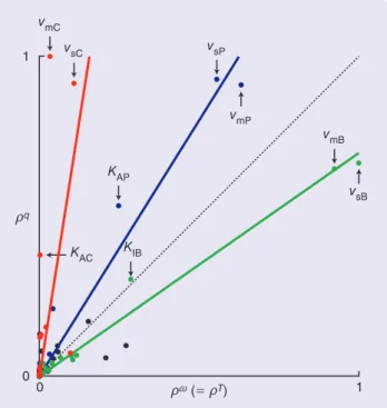
Combining (or not) equivalence properties (9) and (10) ends up with four infinite-dimensional spaces: one Hil-bert space and three quotient spaces, respectively, denoted by QA, QB, QC, and QD (see Table 1). In the next four

sub-sections, each space is endowed with an appropriate Rie-mannian metric and an expression of tangent vectors, needed for the sensitivity analysis in subsequent sections, is provided.

Below, the symbol q denotes an element of the consid-ered space, which can be a signal (a finite or infinitesimal phase-response curve) or an equivalence class of these sig-nals. In the latter case, a signal is denoted by q

_r

.

Metric on Hilbert Space

H1

The simplest space structure is the Hilbert space QA:= H1. The (flat) Riemannian metric on QA is the inner product

( , ) : , gq p gq q =Gp gq qH

with (Euclidean) induced norm

( , ) ,

: g .

q q q q q G q qH _{q 2}

p = p p = p p = p

Because the space QA is a linear space structure, the

short-est path between two elements q1 and q2 on QA is the straight

line joining these elements. The natural (geodesic) distance between two points q1 and q2 on QA is then given by

dist( , )q q1 2 := q1-q_{2 2}.

Metric on the Quotient Space

H1/R>0

The space capturing the scaling equivalence (9) is the quo-tient space QB:=H1/R>0. Each element q in QB represents

an equivalence class

[ ] : { : }. q= qr = qra a> 0

These equivalence classes are rays (starting at zero) in the total space QB:=H1.

The normalized metric on QB,

( , ) : , , _, gq q q _{q q}q q G H G H p g = p g r r r r r r r r r r r r (11) is invariant by scaling. As a consequence, it induces a Rie-mannian metric ( , ) :gq p gq q = rgqr( , )p gr rqr qr on QB. The norm in

the tangent space T Qq B at q is

: g ( , ) _q .

q q q q q q

2 2

p = p p = p_rr ₍₁₂₎

A signal representation of a tangent vector at q!QB

relies on the decomposition of the tangent space T Qqr B into

its vertical and horizontal subspaces. The vertical subspace Vqr is the subspace of T Qqr B that is tangent to the

equiva-lence class [ ],qr that is,

{ :q R}. Vq= rb b!

The horizontal space Hq is chosen as the orthogonal

com-plement of Vqr for the metric ( , ),grqr $ $ that is, { T : ( ,g q ) 0}. Hqr= h! qrQB rqr h rb =

table 1 combining equivalence properties defines different quotient spaces for phase-response curves.

( ) ( ) q $ ?q$a q( )$ +q( )$a ( ) ( ) q$ ?q $+v QA:=H1 QB:=H1 R>0 ( ) ( ) q$ +q$+v QC_:=H1 _{Shift( )}S1 QD:=H1 (R>0#ShiftS1)

The orthogonal projection Pqhrh of a vector h!T Qqr B onto

the horizontal space Hqr is

: _{( ,}( , )_{) ,}, . Pqh _{g q q}g q q _{q q}q q q q G H G H h h b b h b b h h = -_{r r}r r_r r = -r -r r r r r r

The distance between two points q1 and q2 on QB is

defined as dist( , ) :q q1 2 cos 1 _qq q, _q 1 2 2 2 1 2 G H = -r r r r e o

(see [43] for metrics on the unit sphere).

Metric on the Quotient Space

H1/Shift( )S1

The space capturing the phase-shifting equivalence (10) is the quotient space QC:=H1/Shift( ).S1 Each element q in

QC represents an equivalence class

[ ] { ( ): }. q= qr = qr $+v v!S1

These equivalence classes are closed one-dimensional curves (due to the periodicity of the shift) on the infinite-dimensional hypersphere of radius qr ₂ in the total space

. : QC=H1

The (flat) metric on QC

( , ) : , , grrqp gr rqr qr =Gp gr rqr qrH

is invariant by phase shifting along the equivalence classes. As a consequence, it induces a Riemannian metric

( , ) : ( , )

gqp gq q = rgqr p gr rqr qr on QC. The norm in the tangent space

T Qq C at q is

: g( , ) .

q q q q q _{q 2}

p = p p = rrp

The vertical space Vqr is the subspace of T Qqr C that is

tangent to the equivalence class [ ],qr that is, {q : R}, Vq= rlb b!

where qlr has to belong to L2( , )S R1 to ensure the regularity of Vqr. The horizontal space Hqr is chosen as the orthogonal

complement of Vqr for the metric ( , ),grqr $ $ that is, { T : ( ,g q ) 0}. Hqr= h! qrQC rrq h rlb =

The orthogonal projection Pqhrh of a vector h!T Qqr C onto

the horizontal space Hqr is

: ( , ) ( , ) , , . P g q q g q q q q q q q h q q G H G H h h b b h b b h h = - _l l_l l = - _{l l}l l r r r r r r r r r r r r r

The distance between two points q1 and q2 on QC is

defined as dist( , ) :q q1 2 min q1( ) q2( ) ₂ q1( ) q2( ) ,₂ S1 $ $ v $ $ v = - + = - + ) ! v r r r r

where v) denotes the phase shift achieving this

minimiza-tion. It corresponds to the phase shift maximizing the cir-cular cross-correlation ( ), ( ) . arg max q1 q2 S1 $ $ G H v)= +v ! v r r (13)

The global optimization problem (13) is solved in two steps. The first step is the computation of the circular cross-correlation :c Sr 1"R between the two periodic signals q1r and q2r

( ) ( ), ( ) . c v =Gq1 $ q2 $+vH

r r r

By definition, the circular cross-correlation is also a peri-odic signal. An efficient computation of this circular cross-correlation is performed in the Fourier domain. The circu-lar cross-correlation can be expressed as the circucircu-lar convolution ( )c_r v =( ( )q_r1 -$ 9) q_r2( ))( ).$ v _{Exploiting the}

prop-erties of Fourier coefficients and the convolution-multipli-cation duality property leads to

[ ] [ ] [ ], c krt =q1rt k q k)rt2

where [ ]x $

t

denotes the discrete signal of Fourier coeffi-cients for the periodic signal ( )x $, and x) _{denotes the} com-plex conjugate of .x The second step is the identification of the optimal phase-shift value v)!S1, which achieves the maximal value of the circular cross-correlation. This maxi-mum is global and generically unique. Multiplicity of the optimum would mean that one of the signals has a period that is actually equal to /k2r with k!N>0.

Metric on the Quotient Space

H

1

/(

R

>0

#

Shift S

( )

1

)

The space capturing both scaling and phase-shifting equivalences (9)–(10) is the quotient space QD:=H1/(R>0#

Shift( )).S1 Each element q in QD represents an

equiva-lence class

[ ] { ( ) : , }.

q= qr = qr $+v a a> 0v!S1

Based on the individual geometric interpretation of both equivalence properties, these equivalence classes are infi-nite cones in the total space QD:=H1, that is, the union of rays that start at zero and go through the closed one-dimensional curve of phase-shifted signals.

Because the metric (11) on QD is invariant by scaling and

phase shifting along the equivalence classes, it induces a Riemannian metric ( , ) :gqp gq q = rgqr( , )p gr rqr qr on QD. The norm

in the tangent space T Qq D at q is given by (12).

The vertical space Vqr is the subspace of T Qqr D that is

tangent to the equivalence class [ ],qr that is, {q q : , R}. Vqr= rb1+ lr b2 b b1 2!

It is the direct sum of vertical spaces for equivalence prop-erties individually. The horizontal space Hqr is chosen as

the orthogonal complement of Vqr for the metric ( , ),gq$ $

that is,

{ T : ( ,g q q ) 0}. Hqr= h! qrQD rrqh rb1+rlb2 =

The orthogonal projection Pqhrh of a vector h!T Qqr D onto

the horizontal space Hqr is

: ₍( ,_, )₎ ( , ) ( , ) , , , , . P _{g q}g q_q q g q q g q q q q q q q q q q q h q q q q 1 1 1 1 2 2 2 2 G H G H G H G H h h b b h b b b b h b b h h h = - -= - -l l l l l l l l r r r r r r r r r r r r r r r r r r r r r r r r r

The distance between two points q1 and q2 on QD is

defined as

dist( , ) : min cos ( ), ( ) cos ( ), ( ) , q q q _q q _q q q q q 1 2 1 1 2 2 2 1 2 1 1 2 2 2 1 2 S1 $ $ $ $ G H G H v v = + = + ) ! v -r r r r r r r r e e o o

where v) denotes the phase shift achieving this

minimiza-tion. The phase shift v) corresponds to the phase shift maximizing the circular cross-correlation in (13).

SENSITIvITY ANALYSIS IN ThE SPACE

Of PhASE-RESPONSE CuRvES

Sensitivity analysis for oscillators has been widely studied in terms of sensitivity analysis of periodic orbits [44]–[47]. This section develops a sensitivity analysis for phase-response curves. The sensitivity formula and the develop-ments in this section are closely related to those in [48], which studies the sensitivity analysis of phase-response curves, also called perturbation projection vectors, in the context of electronic circuits. The use of sensitivity analysis of phase-response curves is novel in the context of biologi-cal applications.

This section summarizes the sensitivity analysis for oscillators described by nonlinear time-invariant, state-space models with one parameter

( , , ),

xo =f x um (14a)

( , ),

y=h x m (14b)

where the constant parameter m belongs to some subset

. R 3

K The scalar nature of the parameter is for conve-nience but all developments generalize to the multidimen-sional case. See “Basic Concepts of Local Sensitivity Analy-sis” for a short introduction to these concepts.

Basic Concepts of Local Sensitivity Analysis

T

his brief exposition recalls basic concepts of local

sensitiv-ity analysis, following the terminology of [88].

Consider an oscillator described by (14). Most characteris-tics of this system (defined in the previous sections) depend on the value of the parameter .m It means that, for each character-istic of the system, there exists a function :c K"C that associ-ates with each value of the parameter m an element ( )cm in the space C to which belongs the characteristic.

Under appropriate regularity assumptions (see [88] for details), the sensitivity function Sc:K"Tc( )mC of the charac-teristic ( )cm associates with each value of the parameter m the element Sc( )_{m in the tangent space T C}

( ) c m at ( ),cm defined as ( ): ( ) lim ( ) ( ). S c h c h c c h 0 2 2 m m m m m = + -= "

The sensitivity Sc( )_{m provides a first-order estimate of the} effect of parameter variations on the characteristic. It can also be used to approximate the characteristic when m is sufficiently close to its nominal value m0. For small m-m0 2, the

char-acteristic ( )cm can be expanded in a Taylor series about the nominal solution ( )cm0 to obtain

( ) ( ) ( ) .

cm =cm0 +Sc m0 m-m0 2+O^m-m0 22h

This means that the knowledge of the nominal characteristic ( )

cm0 and the sensitivity function suffices to approximate the

characteristic for all values of m in a small ball centered at .m0

The main difficulty of sensitivity analysis is to formulate the appropriate (analytical) equation to be solved to find the charac-teristic ( ).cm Then, differentiating this (analytical) equation yields the sensitivity equation to be solved to find the sensitivity function

( ).

Sc

0

m The analytical problem can be an algebraic problem, an initial value problem, a boundary value problem, etc.

REMARk

If, for a given value of the parameter ,m the characteristic ( )cm is itself a function ( ) :cm A"B in the space of functions ,C the sensitivity Sc( )_{m is also a function S}c_{( ) :m A}

u

_"B

u

_{in the tangent} space Tc m( )C, where A

u

and B

u

are the domain and the image of the sensitivity function. For convenience, the characteristic and the sensitivity function are denoted by :c A#K"B and

: ,

S Ac

u

_#K"B

u

_{respectively.} REMARk

It is often meaningful to compute the relative sensitivity function ( ), c v m defined as ( ) : ( ) ( ) [ ] [ ( ) ( )] ( ) , lim c c h c h c c ( ) ( ) c c h c 0 2 2 v m m m m m m m m m m m = = + -+ -" m m

where $ c( )m denotes the norm induced by the Riemannian

metric gc( )m^ h$ $, at ( ).cm A relative sensitivity function mea-sures the relative change in the model characteristic to a rela-tive change in the parameter value.

Sensitivity Analysis of a Periodic Orbit

The (zero-input) steady-state behavior of an oscillator model (that is, its periodic orbit c) is characterized by an

angular frequency ( ),~ m which measures the speed of a

solution along the orbit, and a 2r-periodic steady-state

solution ( ; )xc $ m =z( / ( ), ( ), , ),$ ~ m x0c m 0m which describes the

locus of this orbit in the state space.

The sensitivity of the angular frequency at a nominal parameter value m0 is the scalar ( )S~m0 !R, defined as

( ): ( ) lim ( ) ( ). S d_d h_h h 0 0 0 0 0 m ~ ~ ~ m m m m = = + -" ~

Likewise, the sensitivity of the 2r-periodic steady-state

solution is the 2r-periodic function Sxc( ; ):$ m0 S1"Rn, defined as ( ; ) : ( ; ) lim ( ; ) ( ; ). Sx dx_d x h_h x h 0 0 0 0 0 $ $ $ $ m m m m = m = + -" c c c c

From (5) and then taking derivatives with respect to ,m

( ; ) ( ; ) ( ; ) ( ; ) ( ) ( ; ) , d dS _{A S v S} E 1 1 1 ₀ x x x 0 0 0 ₂ 0 0 0 i i m ~ i m i m ~ i m m ~ i m - + - = ~ c c c (15a) ( ; ) ( ; ) , Sx 2 Sx 0 0 0 0 r m - m = c c (15b) ( ( ; ); ) ( ; ) ( ( ; ); ) , x x 0 0 0 Sx 0 0 x 0 0 0 0 2 2 2 2 { m m m m { m m + = c c c t t (15c) where ( ; ) : ( ( ; ), , ), ( ; ) : ( ( ; ), , ), ( ; ) : ( ( ; ), , ). A _xf x E f x v f x 0 0 0 x 0 0 0 0 0 0 0 0 0 2 2 2 2 i m i m m i m m i m m i m i m m = = = c c c c

Remark

The sensitivity of the period is often preferred to the sensi-tivity of the angular frequency [46], [49]–[52]. The sensitiv-ity of the period is the real scalar ST

( ) : ( ) lim ( ) ( ). ST dT_d T h_h T h 0 0 0 0 0 m m m m = m = + -"

The sensitivity measures are equivalent up to a change of sign and a scaling factor, that is, ( )/ ( )ST T

0 0

m m =

( )/ ( ). S m0 ~ m0 - ~

Sensitivity Analysis of a Phase-Response Curve

The input–output behavior of an oscillator model is charac-terized by its infinitesimal phase-response curve ( ; ).q $ m

The sensitivity of the infinitesimal phase-response curve at a nominal parameter value m0 is the 2r-periodic

function ( ; ):Sq $ m0 S1"R, defined as ( ; ): ( ; ) lim ( ; ) ( ; ). Sq _ddq q h_h q h 0 0 0 0 0 $ $ $ $ m m = m = m + - m "

From (2) and then taking derivatives with respect to ,m

( ; ) ( ; ), ( ( ; ), , ) ( ; ), ( ( ; ), , ) ( ; ) ( ( ; ), , ) , S S _uf x p _{x u}f x S u f x 0 0 0 q p x 0 0 0 0 0 2 0 0 0 2 0 0 2 2 2 2 2 2 2 2 i m i m i m m i m i m m i m m i m m = + + c c c c

where the 2r-periodic function ( ; ) :Sp $ m0 S1"Rn is the sen-sitivity of the gradient of the asymptotic phase map evalu-ated along the periodic orbit ( )p $ , defined as

( ; ) : ( ; ) lim ( ; ) ( ; ). SP _ddp p h_h p h 0 0 0 0 0 $ $ $ $ m m m m = m = + -"

From (6) and then taking derivatives with respect to m,

( ; ) ( ; ) ( ; ) ( ; ) ( ; ) , d dS _{A S} E p 1 1 ₀ T T p p p 0 0 0 0 0 i i m ~ i m i m ~ i m i m + + = (16a) ( ; ) ( ; ) , Sp 2 Sp 0 0 0 0 r m - m = (16b) ( ; ), ( ; ) ( ; ), ( ; ) ( ) , Sp v p Sv S 0 0 0 0 0 0 i m i m + i m i m - ~ m = _(16c) where ( ; ) : ( ( ; ), , ) ( ; ) ( ( ; ), , ) ( ( ; ), , ) ( ), E _{x x}f x S x f x x f x S 0 0 1 ₀ ij p j k i k x k n j i j i 0 2 0 0 0 1 2 0 0 0 0 0 2 2 2 2 2 2 2 2 i m i m m i m m i m m ~ im m m = + -c c c ~ = c

/

Sv( ; ): _xf( ( ; ), , )x 0 Sx( ; ) f ( ( ; ), , ).x 0 0 ₂2 0 0 0 ₂2 0 0 i m i m m i m m i m m = c c + c

Numerics of Sensitivity Analysis

Numerical algorithms to solve boundary value problems (15) and (16) are reviewed in “Numerical Tools.” Existing algo-rithms that compute periodic orbits and infinitesimal phase-response curves are easily adapted to compute the sensitivity functions of periodic orbits and infinitesimal phase-response curves, essentially at the same computational cost.

APPLICATIONS TO BIOLOGICAL SYSTEMS

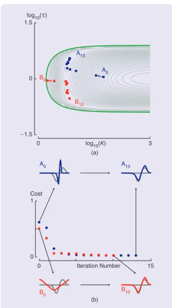
This section illustrates the relevance of sensitivity analysis for three system-theoretic case studies arising from biolog-ical systems, emphasizing the novel insight provided by the approach described in this article with respect to the existing literature. The first application analyzes the robustness to parameter variations of a circadian oscillator model based on the sensitivity of its phase-response curve. The second application identifies the parameter values of a simple circadian oscillator model to fit an experimental-like phase-response curve. The third application classifies