Development and application of a framework for technology and model selection under uncertainty

Development and Application of a Framework for

Technology and Model Selection Under

Uncertainty

by

Ingrid Berkelmans

B.S., University of Melbourne (2002)

B.Eng., University of Melbourne (2002)

ARCHIVES

OF TECHNOLOGY

JUN 3 0 2010

LIBRARIES

Submitted to the Department of Chemical Engineering

in partial fulfillment of the requirements for the degree of

DOCTOR OF PHILOSOPHY IN CHEMICAL ENGINEERING

at the

MASSACHUSETTS INSTITUTE OF TECHNOLOGY

June 2010

@

Massachusetts Institute of Technology 2010. All rights reserved.

A uthor ...

Department of Chemical Engineering

March 12 2010

C ertified by ...

9 ' (gregory J. McRae

Hoyt C. Hottel Professor of Chemical Engineering

Thesis Supervisor

Accepted by ...

William Deen

Professor of Chemical Engineering

Chairman, Committee for Graduate Students

Development and Application of a Framework for

Technology and Model Selection Under Uncertainty

by

Ingrid Berkelmans

Submitted to the Department of Chemical Engineering on March 12 2010, in partial fulfillment of the

requirements for the degree of

DOCTOR OF PHILOSOPHY IN CHEMICAL ENGINEERING

Abstract

Technology selection is a complex decision problem that is often faced in process engineering. This has been a particularly important problem recently in the energy field, in which many new technologies have been proposed. Typically only point estimates of the chosen metrics are used in the evaluation, with uncertainty often overlooked. However, uncertainty can have a significant effect on the conclusions and decisions to be made.

This work investigates the issues surrounding the uncertainty in process engineer-ing models. Model complexity, selection bias and information gain are examined. Existing model selection methods, including Information Criteria Methods and Hy-pothesis Testing are analyzed, with an emphasis on how they address issues surround-ing uncertainty in models. Bayes' methods are investigated in detail because they offer a mathematically sound and very flexible alternative to traditional techniques.

A framework is proposed for evaluating the information difference between

com-peting process engineering models involving uncertainties. This framework can be applied when there are competing processes (e.g. a technology selection problem) or when there are competing models for the one process (e.g. several models of the one process with different levels of complexity). The framework uses the Determin-istically Equivalent Modeling Method (DEMM) and Bayes' model selection methods and consequently can be applied to black box models. The methods chosen allow as-sumptions required in other methods to be relaxed, while keeping computation time minimal. In particular, assumptions about output distributions are relaxed, which is important in process engineering models because equilibrium and theoretical limits can cause output distributions to be highly irregular. A major challenge has been ap-plying Bayes' model selection methods to cases where experimental output data does not exist, which occurs when assessing new technologies. Modifications to existing model selection have been developed to address these cases.

Applying this framework will give the information difference between models, and identify which parameters are driving the overall. These results can be used in a sequential decision making process, facilitating decisions over the best use of resources.

This may include helping to shape experimental programs or further refinement of the models.

The framework has been applied to three case studies. The first involves com-peting hydrogen producing thermochemical cycles. It was found that the best use of resources was to further investigate the separations involved, rather than the reac-tions. The second involved two versions of a refinery process. The overall uncertainty was driven by uncertainty in the fitted parameters, and consequently if a difference is to be observed then the uncertainty in these fitted parameters need to be reduced.

The third case study involved competing technologies for warm syngas cleanup. The excel-based tool has been constructed so that this framework can be applied

by others in the future. This tool calls Matlab to complete the required calculations,

but only requires the user to enter the required inputs in Excel, making it easy for the user.

Thesis Supervisor: Gregory J. McRae

Acknowledgments

The work I have completed could not have been possible without the support of a number of people.

I would firstly like to thank my thesis advisor, Professor Greg McRae. He has given me guidance and support throughout my research. He has been very understanding when I have faced difficulties, and provided direction, motivation and many valuable suggestions throughout my studies. His enthusiasm and patience during my studies have facilitated my progress.

Professor William Green, Howard Herzog and Randall Field have provided much constructive input and helpful suggestions during committee meetings, and I wish to thank them for that.

I would like to thank my colleagues, past and present, in the McRae research lab:

Carolyn Seto, Anusha Kothandaram, Kenneth Hu, Sara Passone, Adekunle Adeyemo, Arman Haidari, Bo Gong, Alex Lewis and Mihai Anton. They have created a friendly and encouraging atmosphere in the lab which I enjoyed.

BP has provided funding for my research. In addition, I have been able to work with various people in BP, gaining valuable insight on how my research can be applied in industry. The members of the MIT-BP Project Team have been a great group of people to work with. In particular I want to thank George Huff for his contributions.

My work has required using models developed by others. Consequently I have been

grateful to those who have supplied models and have been very patient when with me when I needed help when using the models. These people include Bruce Briggs, Linh Quach and Ozie Owen from BP, and David Couling, Zan Liu and Prakash Kshitij from the Professor Green's Group.

Having a family while at completing my PhD has been a challenging task. The staff at TCC have taken great care of my children, allowing me to concentrate on my studies during the day and not worry about my children. In particular I would like to thank Jessie Fernandes and Diane O'Donnell who have been my children's primary carers. The TCC Scholarship program has allowed me to place my children there,

which otherwise would have been financial impossible. The Center for Work, Family and Personal life and the GSC have been valuable resources for me in dealing with balancing my family and my work.

Lastly, I would like to thank my family. My parents Yvonne and William Berkel-mans have been very encouraging throughout my time at MIT. My husband Andrew has been a great support, and my sons Heath and Declan for providing some much needed comic relief at times.

Contents

2.1 Model Fundamentals and Notation 2.1.1 Model Components . . . . . 2.1.2 Probabilty Density Function

2.1.3 M etric . . . . 2.2 Uncertainty in Models . . . . 2.2.1 Model Parameters . . . . . 2.2.2 Model Structure . . . . 2.3 Bayes Theory . . . . 2.3.1 Bayes Rule . . . ... 2.3.2 Likelihood Function . . . . . 2.3.3 Prior Distributions . . . . . 2.3.4 Posterior Distribution . . . 2.3.5 Parameter Estimation . . .

3 Model Selection Methods

3.1 Introduction . . . . . . . .. 7 21 21 21 22 23 25 . . . . 25 (pdf) 25 26 26 29 29 32 33 33 34 35 40 41 45 45

3.2 Frequentist Hypothesis Testing . . . . 46

3.2.1 Null Hypothesis . . . . 46

3.2.2 _{Statistical tests . . . .} 46

3.2.3 A N OVA . . . . 48

3.2.4 Regression and Model Selection . . . . 48

3.2.5 Likelihood Ratio Tests . . . . 50

3.2.6 Lim itations . . . . 50

3.3 Information Criteria Methods . . . . 51

3.3.1 Akaike Information Criterion . . . . 51

3.3.2 Bootstrap Methods . . . . 54 3.3.3 Cross-Validation Methods . . . . 55 3.4 Bayesian Methods . . . . 56 3.4.1 Bayes' Factors . . . . 56 3.4.2 Prior Selection . . . . 57 3.4.3 Evaluation of Integrals . . . . 63 3.4.4 Asymptotic Methods . . . . 65 3.5 Comparison of Methods . . . . 67

3.5.1 Hypothesis Testing and Bayesian Methods . . . . 67

3.5.2 AIC and Bayesian Methods . . . . 68

3.5.3 Bayesian Methods . . . . 69

4 Challenges in Model Selection 71 4.1 Model Complexity... . . . . . 71

4.1.1 Description of Problem . . . . 71

4.1.2 How Methods Address Problem . . . . 73

4.2 Selection Bias . . . . 76

4.2.1 Description of Problem. . . . . .. 76

4.2.2 How Methods Address Problem . . . . 80

4.3 Uncertainty in Model Structure... . . . . . . . 81

4.3.1 Description of Problem . . . . 81 8

4.3.2 How Methods Address Problem . . . . 82

4.4 Information Gain . . . . 83

4.4.1 Distribution of Bayes Factors and Data Set Size . . . . 83

4.4.2 Expected Bayes Factor and Data Set Size . . . . 84

4.4.3 Comparison to Hypothesis Testing . . . . 87

4.4.4 Reaction Kinetics Example . . . . 95

4.5 Sum m ary . . . . 96

5 Framework For Analysis 99 5.1 Introduction . . . . 99 5.2 Uncertainty Propagation . . . . 100 5.2.1 Monte Carlo . . . . 101 5.2.2 D EM M . . . . 101 5.2.3 Method Chosen . . . . 104 5.3 Model Comparison . . . . 104 5.3.1 Available Methods . . . . 104

5.3.2 Bayesian Methods for Technology Selection . . . . 105

5.3.3 Method Chosen . . . . 113

5.4 Model Selection and Resource Allocation . . . . 113

5.4.1 Model Selection . . . . 115 5.4.2 Resource Allocation . . . . 115 5.5 Heuristics... . . . . . . .. . 117 5.5.1 PCE expansion . . . . 117 5.5.2 Termination Criteria... . . . . . . .. 118 5.6 Framework Summary . . . . 119

6 Example: Thermochemical Cycles 123 6.1 Background . . . ... . . . . . . . . . 123

6.2 M ethod . . . . 124

6.2.1 Cycles Examined . . . . 124

6.2.3 Parameters 6.2.4 Model Complexity . . . . 6.2.5 Cycle Comparisons . . . . 6.2.6 Assumptions . . . . 6.2.7 Uncertainty Propagation . 6.2.8 Sensitivity Analysis . . . . 6.3 Initial Results . . . . 6.3.1 Model Complexity . . . . 6.3.2 Comparison of Cycles . . . 6.3.3 Sensitivity Analysis . . . . 6.3.4 H2S Cycle . . . . 6.4 Revised Results . . . . 6.4.1 Separation Work Efficiency 6.4.2 Comparison of Cycles . . . 6.4.3 Discussion . . . .

6.5 Conclusions. . . . ..

7 Technology Selection Example: Warm Syngas Cleanup 7.1 Background . . . .

7.2 Proposed Technologies . . . .

7.2.1 Hydrogen Selective Membrane . . . .

7.2.2 Carbon Dioxide Selective Membrane . . . .

7.2.3 Pressure Swing Adsorption . . . .

7.2.4 Temperature Swing Adsorption . . . .

7.3 M ethod . . . . 7.3.1 CO2 Selective Membrane . . . . 7.3.2 H2 Selective Membrane . . . . 7.3.3 Sorbent Model . . . . 7.4 R esults . . . .. . . . 7.4.1 CO2 Membrane . . . . 10 125 126 126 126 126 128 129 129 129 130 133 133 134 135 137 138 139 139 140 140 140 141 141 141 141 143 143 144 144

7.4.2 H2 Selective Membrane . . . . 7.4.3 Sorbent . . . . 7.4.4 Comparison of Technologies . . . . 7.4.5 Limitations of Models . . . . 7.4.6 Discussion . . . . 7.5 Conclusions . . . .

8 Model Selection Example: Refining Process 8.1 Background . . . . 8.2 Method . . . . 8.2.1 Models analyzed . . . . 8.2.2 Parameters . . . . 8.2.3 Data . . . . 8.2.4 Methods of Analysis . . . . 8.3 R esults . . . . 8.3.1 Inputs . . . . 8.3.2 8.3.3 8.3.4 Fitted Parameters . . . . Contribution of each parameter . Uncertainty in Fitted Parameters 8.4 Conclusions. . . . . . . .. 9 Excel Interface 9.1 Introduction . . . . . .. 9.2 Worksheets . . . ... 9.2.1 Input-data worksheet . . . . 9.2.2 Modelx worksheet . . . . 9.2.3 coef worksheet . . . . 9.2.4 distri worksheet . . . . 9.2.5 Bayes worksheet . . . .

9.3 Procedure for Using Spreadsheet . . . . .

146 146 148 149 150 151 153 . . . . 153 . . . . 154 . . . . 154 . . . . 154 . . . . 155 . . . . 155 . . . . 155 . . . . 155 . . . . 158 . . . . 159 . . . . 160 . . 163 165 165 165 165 167 167 168 169 169

A Thermochemical Cycles Data A.1 Magnesium Iodine Cycle . .

A.2 Copper Chloride Cycle ...

A.3 VCl Cycle ...

A.4 CaBr Cycle ...

A.5 CuSO4 Cycle ...

A.6 Hybrid Chlorine Cycle ...

A.7 KBi Cycle ...

A.8 H2S Cycle ... A.9 SI cycle ... 173 . . . 173 . . . 177 . . . . 181 . . . . 183 . . . . 185 . . . . 187 . . . . 189 . . . . 191 . . . . 193 B Refining Process Data

B .1 D istributions . . . .

197 197

List of Tables

2.1 Possible Metrics to Measure A Process[36] . . . . Statistical Tests Used In Hypothesis Testing . . . . t-Distribution Table . . . . Data for x1, x2 and y . . . .

ANOVA Statistics for Regression Example . . . . ANOVA Statistics for Regression Example for each Parameter 3.6 Classification for

AZ

3.7 AIC values for Example . . . . 3.8 Classification for Bayes Factors . . . . .

3.9 Bayes Factors Using Several Priors . . .

4.1 Coefficients and Functions . . . . 4.2 Properties of Method Selection Methods

Orthogonal Basis Polynomials[54] . . . Classification of dissimilarity of 2 distribu

PCE coefficients and . . . .

Methods Implemented in Framework . .

. . . . 27 . . . . 47 . . . . 47 . . . . 49 . . . . 49 . . . . 50 . . . . 5 2 . . . . 54 . . . . 5 6 . . . . 6 2 . . . . 7 7 . . . . 9 7 .... ... . . . .. 102 Lions . . . . 106 . . . . 116 . . . . 12 1

6.1 Thermochemical Cycles Examined . . . .

6.2 Base Values and Standard Deviations of Parameters . . . .

6.3 Levels of Analysis . . . .

6.4 Modified KL distance for Thermochemical Cycles using results from F igure 6-2 . . . . 3.1 3.2 3.3 3.4 3.5 5.1 5.2 5.3 5.4 125 127 128 130

6.5 Bayes Factors for Thermochemical Cycles using results from Figure 6-2 6.6 Parameters with Largest Contribution to Variance of Overall Efficiency

6.7 Contribution to overall variance of most significant parameters . . . .

6.8 Modified KL distance for Thermochemical Cycles using results from

F igure 6-6 . . . .

6.9 Bayes Factors for Thermochemical Cycles using results from Figure 6-6 7.1 Uncertainty in Input parameters for CO2 Selective Membrane

7.2 Collocation Points for Model Evaluations... . . . . ..

7.3 Uncertainty in Input parameters for Sorbent Model . . . .

7.4 PCE coefficients . . . .

7.5 PCE coefficients . . . .

7.6 PCE coefficients for Sorbent Model . . . .

7.7 Bayes Factors . . . . 8.1 Input parameters. . . . . . . . .. 8.2 Bayes Factors of Outputs . . . .

8.3 Classification of Model Differences . . . . 8.4 First Order PCE coefficients . . . .

8.5 PCE coefficients... . . . . . . . ..

A. 1 MgI Cycle Reactions... . . . . . . . . ..

A.2 MgI Cycle Energy Requirements... . . . . . . ..

A.3 MgI Cycle Efficiency Calculations... . . . . . . ..

A.4 Sensitivity Analysis Results for MgI Cycle . . . .

A.5 CuCl Cycle Reactions.... . . . . . . ..

A.6 CuCl Cycle Energy Requirements . . . . ... . . . ..

A.7 CuCl Cycle Efficiency Calculations.... . . . . . . . ..

A.8 Sensitivity Analysis Results for CuCl Cycle... . . . . . ..

A.9 CuCl 3 Step Cycle Reactions.. . . . . . . . ..

A.10 CuCl 3 Step Cycle Energy Requirements

14 130 131 132 136 136 . . . . 143 143 144 146 146 148 149 154 156 156 160 161 173 175 176 176 177 178 178 179 179 . . . . . . . . . . . 179

A.11 CuCl 3 Step Cycle Efficiency Calculations . . A.12 CuCl 4 Step Cycle Reactions . . . .

A.13 CuCl 4 Step Cycle Energy Requirements . . .

A. 14 CuCl 4 step Cycle Efficiency Calculations . . .

A.15 VCl Cycle Reactions . . . . A. 16 VCl Cycle Energy Requirements . . . .

A.17 VCl Cycle Efficiency Calculation . . . .

A. 18 Sensitivity Analysis Results for VCl Cycle . .

A.19 CaBr Cycle Reactions . . . .

A.20 CaBr Cycle Energy Requirements . . . . A.21 CaBr Cycle Efficiency Calculations . . . . A.22 Sensitivity Analysis Results for CaBr Cycle . .

A.23 CuSO4 Cycle Reactions . . . .

A.24 CuSO4 Cycle Energy Requirements . . . . A.25 CuSO4 Cycle Efficiency Calculations . . . . .

A.26 Sensitivity Analysis Results for CuSO4 Cycle .

A.27 Hybrid Chlorine Cycle Reactions . . . .

A.28 Hybrid Chlorine Cycle Energy Requirements A.29 Hybrid Chlorine Cycle Efficiency Calculations A.30 Sensitivity Analysis Results for HCl Cycle . A.31 KBi Cycle Reactions . . . . A.32 KBi Cycle Energy Requirements . . . . A.33 KBi Cycle Efficiency Calculations . . . .

A.34 Sensitivity Analysis Results for KBi Cycle . .

A.35 H2S Cycle Reactions . . . .

A.36 H2S Cycle Energy Requirements . . . .

A.37 H2S Cycle Efficiency Calculation . . . .

A.38 Sensitivity Analysis Results for H2S cycle . . .

A.39 SI Cycle Reactions . . . .

A.40 SI Cycle Energy Requirements . . . .

15 . . . . 180 . . . . 180 . . . . 180 . . . . 181 . . . . 181 . . . . 182 . . . . 182 . . . . 183 . . . . 183 . . . . 184 . . . . 184 . . . . 185 . . . . 185 . . . . 186 . . . . 186 . . . . 187 . . . . 187 . . . . 188 . . . . 188 . . . . 189 . . . . 189 . . . . 189 . . . . 190 . . . . 190 . . . . 191 . . . . 192 . . . . 192 . . . . 193 . . . . 193 . . . . 194

List of Figures

2-1 Results of 4 process (A,B,C,D) for 2 metrics (y1, y2) . . . . 28

2-2 Probability Distribution Functions of Parameters and Model Predictions 29 2-3 Probability Density Function of y . . . . 31

2-4 Likelihood Function for - . . . . 37

2-5 Likelihood Function for log(o) . . . . 37

2-6 Likelihood Function for

and sin

_{/# . . . .}

₃₉

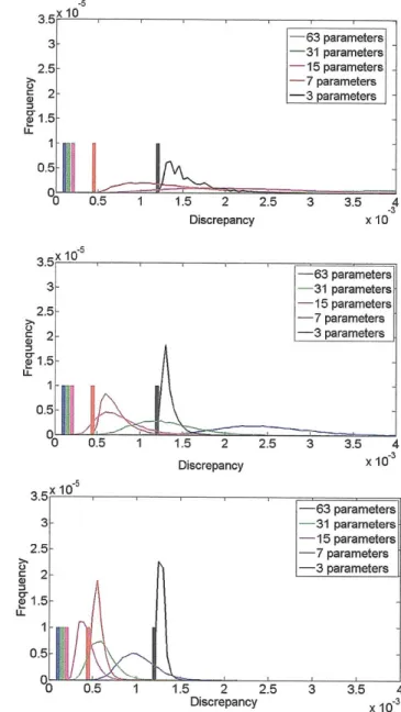
4-1 Student Scores on Test ... ... 72

4-2 Approximating Histograms . . . . 73

4-3 Discrepancy for 50, 200 and 500 data points . . . . 74

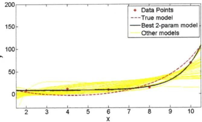
4-4 True and Fitted Approximating Models for Generated Data Points. . 78 4-5 Square Distance from True Model . . . . 78

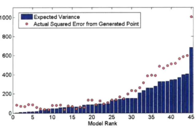
4-6 Predicted Variance and Actual Squared Error for Generated Point at x=3... ... 79

4-7 Best Model with 5 Indicator Variables.. . . . . . . . . 80

4-8 Best Model using AIC . . . . 80

4-9 Distribution of Highest R2 value for a Model with 5 Indicator Variables 81 4-10 Effect of Data Set Size and Bayes Factor PDF . . . . 84

4-11 Expected Strength of Classification . . . . 86

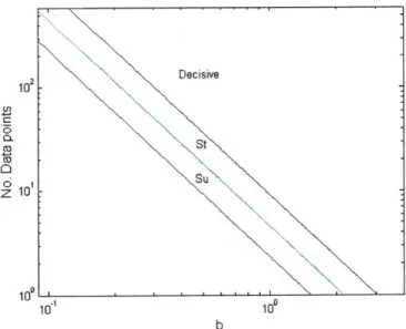
4-12 Strength of Evidence and Expected Data Set Size Required . . . . 87

4-13 PDF of p-values for y = 0.25 . . . . 88

4-14 PDF of p-values for y = 0.75 . . . . 89

4-16 PDF of Bayes Factors . . . . 92

4-17 PDF of Bayes Factors using 8 Data Points . . . . 93

4-18 PDF of Bayes Factors using 8 Data Points . . . . 94

4-19 Prior Knowledge of Half Life . . . . 95

4-20 Prior Knowledge of Rate Constants for ki (left) and k2 (right) . . . . 95

4-21 PDF of Bayes Factors using varying number of data points . . . . 96

5-1 Flow Chart of Framework Steps . . . . 99

5-2 Strength of Classification for 2 Normal Distributions - Method 1 . . . 107

5-3 Examples of each Classification . . . 108

5-4 Probability distribution of M1 and M2 . . . 108

5-5 Strength of Classification for 2 Normal Distributions - Method 2 . . . 111

5-6 Strength of Classification for 2 Normal Distributions - Method 3 . . . 113

5-7 Examples of each Classification . . . 114

5-8 Efficiency of Technology A and Technology B . . . . 116

5-9 Flow Chart of Framework . . . . 120

6-1 Schematic Diagram of Hydrogen Producing Thermochemical Cycle . 124 6-2 Probability Distribution Functions of Efficiency . . . . 129

6-3 Probability Distribution Function for H2S cycle and H20 (using CuC1 intermediates).. . . . . . . . 133

6-4 VCl Cycle Efficiency Probability Distribution Function . . . . 134

6-5 Probability Distribution Functions of Efficiency with Lower Separation Efficiency for Reverse Deacon Products . . . . 135

6-6 Probability Distribution Functions of Efficiency assuming a Uniform Separation Efficiency Distribution.. . . . . . . . 136

7-1 Correlation of Selectivity and Permeability [24]... . . . . 142

7-2 PDF of Percentage of H2 Permeating through Membrane.. . ... 145

7-3 Distributions of Power Loads for CO2 Selective Membrane . . . . 145

7-5 Distributions of Power Loads for Sorbent . . . .

7-6 Net Power from Warm Syngas Cleanup Technologies . . . .

8-1 Examples of each Classification . . . . 8-2

8-3

8-4

8-5

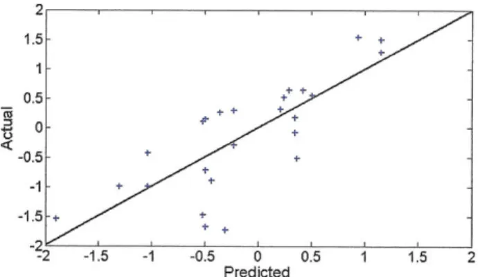
PD Fs of ouputs . . . . PDFs of outputs including uncertainty in fitted activities . . . . PDF of Fitted Activity 1 . . . . PDF of Parameter F with current Fitted Activity 1 (left) and reduced

147 148 157 158 159 160 uncertainty (right) . . . .

8-6 Calculated Fitted Activity 1 and Product 9-1 9-2 9-3 9-4 9-5 9-6 Input-data worksheet Model x worksheet . coef worksheet . . . . . distri worksheet . . . . Bayes worksheet . . . . Flowchart of procedure . . . . 162 Composition . . . . 163 . . . . 1 6 6 . . . . 1 6 7 . . . . 1 6 8 . . . . 1 6 9 . . . . 1 7 0 . . . . 1 7 1 A-1 MgI Cycle Pinch Analysis . . . . A-2 CuCl Cycle Pinch Analysis . . . . A-3 VCk Cycle Pinch Analysis . . . . A-4 CaBr Cycle Pinch Analysis . . . . A-5 CuSO4 Cycle Pinch Analysis . . . . . A-6 Hybrid Chlorie Cycle Pinch Analysis A-7 KBi Cycle Pinch Analysis . . . . A-8 H2S Cycle Pinch Analysis . . . . A-9 SI Cycle Pinch Analysis . . . . A-10 SI Cycle Pinch Analysis . . . . B-1 PDFs of outputs with set tuning factors - A B-2 PDFs of outputs with set tuning factors - B B-3 PDFs of outputs with set tuning factors - C . . . . 174 . . . . 178 . . . . 1 8 1 . . . . 184 . . . . 186 . . . . 188 . . . . 190 . . . . 1 9 1 . . . . 194 . . . . 195 . . . . . . . . . . 198 . . . . 199 . . . . 200

B-4 PDFs of outputs including uncertainty in Activity Factors - A . . . . 201 B-5 PDFs of outputs including uncertainty in Activity Factors - B . . . . 202 B-6 PDFs of outputs including uncertainty in Activity Factors - C . . . . 203

Chapter 1

Introduction

1.1

Motivation

Technology selection is a complex and multi-criteria decision problem that is often faced in process engineering. This has been a particularly important problem recently in the energy field, in which many new technologies have been proposed.[40, 43] This has been due to concerns about the global climate impacts and long term availability of existing energy sources.

Typically in technology selection only point estimates of the chosen metrics are used in the evaluation, with uncertainty often overlooked. However,uncertainty can have a significant effect on the conclusions and decisions to be made. [25] Even when an uncertainty analysis is done, it usually involves methods which have embedded assumptions. The validity and effects of the assumptions are often not addressed. In addition, uncertainty in parameters is usually considered the only source of uncer-tainty, with sources such as uncertainty in model structure not analyzed.

1.2

Aim of work

The aim of this work is to provide a framework to assess new and existing technologies. This involves developing a practical and statistically defensible way to compare pro-cess engineering models. The challenges involved with model selection and model use

under uncertainty are considered. Bayesian methods are explored in detail because these methods, unlike many popular traditional approaches, do not have restricting assumptions, and offer a flexible and powerful way of addressing model uncertainty problems.

1.3

Overview of work

This work investigates model selection under uncertainty. In particular, the uncer-tainty in the inputs of a model are studied. The primary problem considered is evaluating competing technologies, each represented by a model. A secondary model selection problem is also present, which is model selection for a particular process. For example, selecting a model from several models with differing levels of complex-ity. This may involve an existing process where output data exists. For example, one may know output concentrations of chemical species from a reactor and need to choose from a set of models, each consisting of a series of chemical reactions. Much theory has been developed for this type of case. Another case is where the process is proposed, but as yet does not exist. An example is a proposed thermochemical cycle for production of hydrogen, but large scale production does not exist. Much less literature has focused on these types of problems.

This work investigates the issues of determining the uncertainty in complex mod-els, which are common in process engineering. Traditional methods either have re-stricting assumptions or require excessive computation. After the uncertainty has been established, the model selection problem arises. This work analyzes various model selection techniques, in particular looking at how they can be applied when no output data exists, as is the case in many technology selection problems.

Bayesian techniques are investigated in detail because they offer a mathemati-cally sound and very flexible alternative to traditional techniques. Difficulties involv-ing computational intensity and subjectivity of Bayesian methods, which initially slowed the acceptance of these methods, have been mostly overcome for parameter estimation problems. The resolutions to these difficulties can be extended to model

selection problems, but new challenges arise. Addressing challenges unique to model selection problems is a major part of this work. A framework for model selection under uncertainty is proposed. This is applied to three major case studies.

1.4

Outline of Thesis

The thesis can be divded into three main sections: background investigation of model selection methods and issues (Chapters 2-4), proposed framework (Chapter 5) and

case studies (Chapters 6-8).

Chapter 2 contains background theory, introducing model fundamentals and the notation which is used throughout the thesis.

Chapter 3 investigates each model selection method. Hypothesis testing, Infor-mation criteria methods and Bayesian methods are analyzed and compared.

Chapter 4 investigates the challenges in model selection. Model complexity, selec-tion bias, uncertainty in structure and informaselec-tion gain issues are explored through various examples. In addition, the way various model selection methods address these issues is studied.

Chapter 5 explores how model selection methods, and in particular Bayes methods, can be applied to technology selection problems which do not necessarily have output data available. It concludes with the proposed framework.

Chapter 6 applies the framework to a technology selection problem. This exam-ple involved comparing various proposed hydrogen-producing thermochemical cycles. The focus in this case study was to identify the most promising cycles, and to deter-mine the best use of resources for further work.

Chapter 7 applies to framework to several warm syngas cleanup technologies. Various technologies have been proposed to avoid the energy penalty associated with cool syngas cleanup processes, such as Selexol. These technologies have significant uncertainties because none have been implemented on an industrial scale.

Chapter 8 applies the framework to a refining process model. One model is an updated version of the other, with improvements made to the kinetics. Consequently

the two models are of similar complexity. The analysis looks at whether there is any information difference in the predictions of the two models.

Chapter 9 describes the excel tool created to implement the framework. This will enable other researchers to apply to framework to other problems, without necessarily having to be familiar with all the methods of the framework.

Chapter

Background Theory

This chapter covers model fundamentals, notation, model uncertainty and Bayesian theory. This chapter only gives the background theory without any discussion on model selection, which is introduced in Chapter 3.

2.1

Model Fundamentals and Notation

This section introduces model fundamentals and the notation which will be used.

2.1.1

Model Components

A model, M, typically consists of an output (y), inputs (x), parameters (6) and error

(e) where

M: y=h(x;6)+e

Example

(2.1)

Consider the model M representing a series of chemical reactions. Then the components of M could be

9 The output y is the measured concentration of a chemical compound " The parameters 6 are the rate constants of the involved reactions

* The inputs x are the initial concentrations of all chemical species * The error c is the measurement error of the equipment used

A model may have a vector output y instead of a scalar. The components of the

vector may be the same quantity resampled multiple times (eg from the same repeated experiment) or different quantities (eg concentrations of several compounds).

Uncertainty in the parameters 0 and model structure h(-), along with the error e, all contribute to uncertainty in the model output y. A probability density function

(pdf), f(y), can be constructed to describe the spread of the output.

2.1.2

Probabilty Density Function (pdf)

A probability density function (pdf) is defined such that the probability that the true

value of z is within a region A is given by

P(z

E

A)=

j

f(z)dz

Example If z can take on any value between 0 and 1, with each value equally likely

then

1 if 0 < z <1

f (z =

0 otherwise

Normal Distribution It is often assumed that a distribution is normal, especially

when there is a lack of data. A one dimensional normal distribution is given by

1 -p

f(z) = _ e

where y and o- are the mean and standard deviation respectively. The normal distri-bution is often written as z ~ N(p, a2_).

2.1.3

Metric

A metric (or metrics) is required to compare processes. The metric is typically the

output of a model.

Metrics need to be carefully defined, with the consequences of any assumptions of simplifications in the definition considered. For example, thermal efficiency can be

used for a chemical process

-=

(2.2)

Q

where T, is the efficiency of the work processes (e.g. separation work). Different

sep-arations can have vastly different efficiencies. Consequently substantial uncertainty could result if the efficiency is assumed the same for all separations.

Multiple Metrics

Often there is more than one metric of interest. For example, one is unlikely to consider solely environmental indicators without any consideration to cost. Lapkin et

al

[36]

process. Lapkin classifies each metric into one of four areas: society, company and product, infrastructure and process. These are shown in Table 2.1, with examples of different metrics for each area. Afgan et al [2] also considers four areas when assessing energy alternatives. These are resource, environmental, social and economic.

Area Description Example of metric

Society Climate Changes, Release of green house gases

Continuous availability Energy efficiency of energy

Infrastructure Footprint and resource Sustainable process index efficiency

Company Overall environmental Production efficiency

efficiency

Product and Process Maximum use of feed Mass efficiency Minimum use of energy Energy efficiency Table 2.1: Possible Metrics to Measure A Process[36)

There are various methods to evaluate a process or technology when multiple metrics are considered. Lapkin simply lists the value of each metric for each of the process.

Pareto Optimization Approach Pareto optimization is another approach for

considering multiple metrics. A case is considered optimal in a Pareto sense if no metric can be improved without a negative effect on another metric. For example,

consider the case where processes A,B,C and D are being compared using two metrics

yi and Y2, shown in Figure 2-1. In this example, processes A,B and C are Pareto

optimal. However, point D is not Pareto optimal since B is an improvement over D in both y1 and

Y2-4 + 3- A + Y2 2B 1- + 00 1 2 3 4 5 y₁

Figure 2-1: Results of 4 process (A,B,C,D) for 2 metrics (y1, y2)

A Pareto optimization approach was taken by Hoffmann et al[30), where total

annualized profit per service unit (TAPPS) and material intensity per service unit (MIPS) are used. TAPPS is an economic metric that measures the potential maxi-mum profit per unit of product. MIPS is an environmental metric which measures the total material and energy throughput over the life cycle.

Other Approaches A more sophisticated approach is used by Afgan [2]. Four

metrics are considered to compare several energy sources. To construct the multi-objective metric

Q,

where wi and yi,j are the weight and value ith metric respectively, for alternative

j.

This information is then used to determine a probability distribution for the weights, and hence a probability distribution for the resulting multi-objective metric

Q.

2.2

Uncertainty in Models

Uncertainty in predictions from a model can be caused by uncertainty in the values of the parameters and uncertainty of the structure of the model.

2.2.1

Model Parameters

Model parameters will typically not be known precisely. There will be uncertainty in the value of the parameters 6, which will result in uncertainty in the value of the output y. The propagation of uncertainties in the parameters to the model predictions is illustrated in Figure 2-2. (N 0 02 Model -- 1, Calculations Y

Figure 2-2: Probability Distribution Functions of Parameters and Model Predictions

The probability distribution of a model output is given by

f(y|6)f(6)dO (2.3)

where

f(yjG)

then f(y) and

f(y|6)

f(y Ix)

Example Consider the model M where

M : y = 01 + C

... ::::::.. It " - - - - .. ... ...

-f (y)

₌

_j

Then f(y|61) - N(0₁, 1). If 01 has the distribution 01 ~ N(1, 1) then it follows

f(y)

f(y61)f(61)dO1

I

/

Determining Uncertainty from Parameter Uncertainty

An analytic form of the output distribution given by equation (2.3) only exists in special cases. Consequently, numerical methods are usually required to estimate

f(y). A popular method is Monte Carlo simulations, which involves the following

steps:

" Generate a parameter set and calculate the corresponding model output.

" Repeat the generation of parameter sets and model calculations until a sufficient

number of samples is obtained.

" Construct a distribution of the outputs.

There are various methods available for generating the sequence of parameter sets. A crude Monte Carlo method is the simplest. This involves generating each parameter set independently, based on the probability distribution of 6.

Example Consider the model M where

M:y=91 +E ee~N(0,1)

where 01 ~ N(1, 1). A value of 01 is randomly selected from the distribution N(1, 1). The value of y is then calculated, with e randomly selected from N(O, 1). This is repeated many times. Figure 2-3 gives the calculated approximate distribution when using 100 and 1000 instances of 61 and the exact analytical distribution.

When many parameters or nonstandard regions are involved then a crude Monte Carlo method can be computationally expensive and the results may not be accurate.

Figure 2-3: Probability Density Function of y

A more efficient method of traversing the sample space is required. More efficient

methods include the Metrolis-Hastings algorithm [16] and Gibbs sampling [52] gen-erate the next parameter set by using the previous parameter set.

Contribution of Each Parameter

It is often useful to calculate the contribution of each parameter to the overall variance. The total variance of an output y can be expressed as

k

a =

s8oa

+

j=1

where sj is sensitivity of the output on the

jth

(2.4)

Si =

Therefore the first order contribution of each parameter towards the total variance is

Si U0.

The sensitivity of each parameter can be estimated by modifying the parameter slightly and observing the change in the output

Si ~ Ay/A63

2.2.2

Model Structure

There is often uncertainty in the structure of the model ie the form of h(-) and e in Equation 2.1. This is often overlooked. However, the effects of ignoring this uncertainty can be significant. [22]

Model averaging is a method which is gaining popularity to account for model structure uncertainty. [48] This involves assigning a probability P(Mi) to each model

Mi. An estimate of the output yeet can be obtained by using n

Yest = yP(M)W

where y(') is the estimated output from Mi. A probability distribution of y can be obtained by using

n

f(y) = Zfi(y)P(M)

where fi(y) is the pdf of y based on Model i.

Structural uncertainty can also be incorporated in a model. [22] For example, consider the model

M : y, = y + Ej

where c is IID symmetric about zero, but the actual structure is not known. Setting

f(Ela)

(

gives the double exponential distribution for a = 1, the Gaussian for a = 0, the

uniform as a -+ -1, and various distributions for other a. Therefore

f(y) = f(yIp, a)f(p, a)dpda

or in general

f(y)= f(y|6, S)f(6, S)dOdS

assumptions S.

2.3

Bayes Theory

This section describes Bayesian theory in detail. It covers Bayes' rule, the distribu-tions involved and how Bayesian techniques can be applied to parameter estimation problems. Bayesian techniques for model selection are discussed in Chapter 3.

2.3.1

Bayes Rule

Bayesian techniques are based on Bayes' rule, which relates the conditional probabil-ities of two events:

_ P(B|A)P(A)

P(B)

Bayes' rule can be used in the continuous case to give

f

(6|y)

=

(2.5)

f(y)

It is often more convenient to express this as

f (O|y) oc L(6|y) 7r(6) (2.6)

Posterior Likelihood Prior The probability density functions involved are

" Prior Distribution r(6) (or f(0)). This contains the prior knowledge about the

probability distribution of the parameters.

" Likelihood L(O|y). This is the pdf of the data, y, given a value of the parameter

set 0 ie L(6|y) =

f(y|1).

y is usually fixed.

" Posterior

f(G|y).

Bayesian methods require the input of the prior, 7r(6). Therefore the probability dis-tribution of the parameters need to be estimated. The subjectivity involved in choos-ing r(8) and the computation required initially slowed the acceptance of Bayesian methods. Development of methods to construct objective priors, and computational methods that make the calculations required manageable, has meant that Bayesian methods have steadily grown in popularity. [6]

The Bayesian framework can be extended quite naturally beyond inductive infer-ence to analyzing uncertainty in model structure and model selection. Consequently it can be used to tackle problems which traditional approaches can not solve adequately.

2.3.2

Likelihood Function

The likelihood is the probability distribution of the data conditional on the parame-ters. However, 6 is the argument, since the data is fixed i.e.

L(6|y) = fI(y6)

Equation (2.6) is a proportionality relationship and consequently only a term propor-tional to the likelihood is typically required. Therefore multiplicative constants can been removed. The likelihood is determined by the model chosen.

Example Consider the model

M : yi ~ N(p, oa2)

where y2 is the ith data point. Assume that standard deviation o is known and the mean p is unknown. This case may arise when measuring an unknown quantity 0 and the measurement error is known to be normally distributed with a standard deviation

of o. This gives

L(ply, -)

f

= 1 exp - 2

oc exp

-9)2

2 a-w/

2.3.3

Prior Distributions

Prior distributions of the parameters are required when applying Bayesian techniques. If there is prior knowledge about the parameter then this knowledge can be used to estimate the distribution. Alternatively a noninformative prior can be used.

Noninformative Priors

Often there is a desire not to introduce bias or subjectivity into the analysis, or there is a lack of prior information. Using non-informative priors 7N(6) is a way to ensure objectivity. A noninformative prior allows the calculated posterior distribution to be dominated by the data rather than the prior distribution.

Example Consider the model

M: y _{~ N(p, o.}2₎

where both p and o- are unknown parameters. It can be shown that noninformative priors for y and o- are

7N(p) C FN (U) - U (2.7)

where c is some constant. [8]

The priors for the example above are improper (i.e. f grN(p)dy = oo). However, this is generally not a problem since the posterior distribution will still be proper. The posterior can then be normalized if desired.

One may naively predict that a noninformative prior should always be a constant. However, the idea that a uniform prior can be used to represent ignorance is not

self-consistent. A change of variables can be used to prove this (e.g. k = P1-). Instead,

a prior distribution which ensures the likelihood curve is data translated (which may require a transformation) should be used.

Data Translated Likelihoods A data translated likelihood is a likelihood whose

curve is completely determined a priori, except for its location which is determined

by the data. The parameter may need to be transformed

#(O),

corresponding to

#(O)

#(6))

[3]

Example Consider the model

M : yj ~ N(p, o.2)

where p is known and o is unknown. This case may arise when measuring a known quantity p, but standard deviation of the measurement, o, is unknown. The likelihood in this case is

L(-|p, y)

oc or--

exp

(

n

(2.8)

The shape of the likelihood curves, as shown in Figure 2-4, vary with different data.

If the likelihood curves are plotted in terms of log(o) then the curves are data

trans-lated, as shown in Figure 2-5.

The noninformative prior in this case should be uniform in log(O), which gives

7WN (U )o(d log o-do

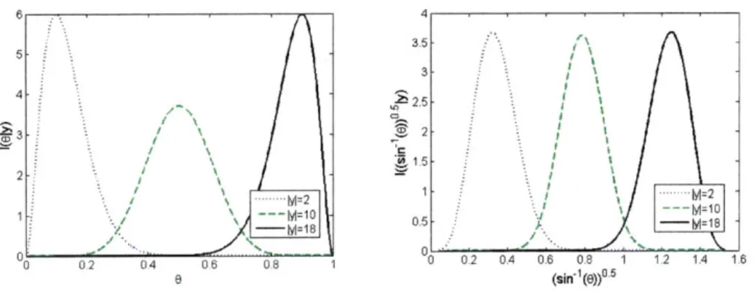
Approximate Data Translated Likelihood Exact data translated likelihoods only exist in special cases. Jeffreys' rule can be applied to construct a prior so that

0.018 0.016 s=2 - -- s=4 0.014 -s8 0.012 0.01 0.008 0.006 I 0.004 0.002 0 0 2 4 6 8 10 12 14 16

Figure 2-4: Likelihood Function for a

1.2 - 00.8-0.6 0.4 0.2 0 -0 1.5 log(e)

Figure 2-5: Likelihood Function for log(a) ...

the likelihood is approximately data translated in cases when you are considering n identical trials e.g. taking n measurements of some quantity.

Definition: Jeffreys' Rule Jeffreys' rule states that a prior distribution for 9

is approximately noninformative if it proportional to square of Fisher's information measure 1(6) where I(6) is defined as

T(9) = -E '82 log L(91yi) ₁ ~

where yj is the result of the ith trial [8].

Example Consider n independent trials, with the probability of success (yj = 1)

being 9. An example of this is n tosses of a biased coin. The distribution for each trial is

L(9|y.) = yi (1 - 6)(yi), yj = 0, 1

Therefore we have

a2 log L(|yi) y 1 - yj

892 92 (1 - g)2

Since E[yf 9|] = 9 then we have

1 1 1

9 (1-9) 9(1-0)

The noninformative prior distribution is therefore

7N(0) = ()- 0-1/2(1 - >1/2

and the transformation required is

#(0)

35 5 -. 3 4 2 21- 5 22 M=2 1 - M=10 1:\ - 18 0.5 _M1 C -0 0.2 06 0.8 1 0 0.2 04 0.6 0.8 1 1.2 1.4 1.6 8 (sin-1(e))0.5

Figure 2-6: Likelihood Function for 9 and sin-1

VF

Jefferys' Rule Derivation The proof of Jeffrey's rule is quite involved. Conse-quently a rough outline of a derivation, and not a rigorous proof, is provided here.

Consider yi, ... y, which are sampled from a distribution f(yj|1) = L(0|yi). If

the distribution obeys certain regularity conditions and n is sufficiently large then the likelihood function is approximately normal. Consequently, the logarithm of the likelihood function is approximately quadratic.

A(91y) = log l(O|y)

n (, _2 1 a2 A

A(O|y)

-

)

,

arg max A(1y)

(2.9)

2 n _502

1 a2A c xmtd t

The term - can be approximated with 1($) where

E

log

L(0|yi)

1

I() 0-982 lv

For any transformation

#5(9)

(d6

I(#) =1() -(2.10)

If

#

do

then from Equation (2.10) it can be seen that I(#) will be a constant and independent

of

#.

#

Extension to Multiparameter Models Jeffreys' Rule for multiparameter

prob-lems states that the prior distribution is taken to be proportional to the square root of the determinant of the information matrix. i.e.

7r(6) C T |1(6) 1/2

where

In(6)

=

E

{

-where A is the logarithm of the likelihood function i.e. A(O|y) = log L(6|y). [8}

Example Consider the case where there is n independent trials, and each trial has

m different outcomes. The probabilities of each outcome is denoted by A,, A2, ... Am.

Let yj denote the number of outcomes of type i. We then have

L(Ay) =1! . . .

This gives A(7rIy) =

Z

|1En(7)1 = n (A, .2 ...

Am)-giving the prior

PN(7r) OC (7ir 2 .. 7m)-1/2

2.3.4

Posterior Distribution

A distribution proportional to the posterior distribution is obtained by multiplying the

likelihood and prior distribution (from Equation (2.6)). This curve can be normalized to give a posterior distribution.

Example Consider the model

M: yj ~ N(p, a-)

where p is known and o is unknown. Then, using the likelihood form Equation (2.8), gives f(o-|p,y) oc L(o-p,y)7r(o-p) n(rs2 o c -"exp~ _2o.2) o--(n+1) exp ( S f , ( o )t I -t (n + ) e x p ( -o d i ep2t2

)d

The normalizing integral can be computed numerically. However, in this example an analytic solution exists

(ns 2)n/2 -_(n+1) ex n 2

f (ojt Y) - 2(n/2)-'F(n/2) e 20 2)

2.3.5

Parameter Estimation

Bayesian techniques allow assumptions required for other techniques to be relaxed when performing parameter estimation. Bayesian methods allow prior knowledge about the parameters and the form of the noise term to be incorporated. Equation

(2.6) is used to calculate the posterior distribution f(y|0). Once the posterior

dis-tribution has been established, the optimal parameter set, O0pt, can then be found. There are various criteria which can be used. For example, the most probable (the maximum of the posterior) could be used. [41].

Other criteria can be considered using a Bayes cost function. This requires the use of a cost function c(6) which fulfills the properties

" If |6i| > |6jI then c(62) > c(0₃)

The Bayes cost function is then defined using the cost function

B(5|x) E

[c(8

-

5)

J

-

5)L(8|y)dO

The value of 0Opt is then found by minimizing the Bayes cost function.

[8]

e Weighted sum of squared error.

c(O) =OTWO, W >_ 0

* Uniform cost function. This cost function maximizes the probability that 0

oPt

is within 6 > 0 of true value of 0.

c(O)

f

0 if |0|<6

1 otherwise

Relationship between Least Squares and Bayesian Methods

A least squares method has traditionally been employed to use the data to estimate parameter values. This method determines which parameter values will minimize the

sum of the square of the differences between the model prediction and the data. For a nonlinear model

M : y = h(x; 6)

+

the optimal parameter set 0Opt when using least squares is

N 0

OPt = arg min (yk - h(xk; 0))2

k=1

where k denotes the kth set of data.

The least squares method is equivalent to the Bayesian approach if * Model is linear

Chapter 3

Model Selection Methods

This chapter focuses on looking at the different types of model selection methods. This is followed by comparisons of the methods which have been made in model selection literature.

3.1

Introduction

There are three main model selection methods: frequentist hypothesis testing, infor-mation criteria methods and Bayesian methods. Hypothesis testing involves propos-ing a hypothesis and uspropos-ing data to test it. Information criteria methods are based on selecting a criterion to compare models and then calculating an estimation of the selected criterion for each model using the data available. Both hypothesis testing and information criteria methods methods are quite popular. However they often contain embedded assumptions. The validity and effects of the assumptions are often not addressed. Bayesian methods offer an attractive alternative. Bayesian methods are based on implementing Bayes' rule, and make no assumptions about the types of distributions involved. The assumptions necessary for conventional statistical theory can often be relaxed for Bayesian approaches.

3.2

Frequentist Hypothesis Testing

Frequentist hypothesis testing techniques are often employed in model selection prob-lems. These techniques are often chosen simply because of the ease of application and the familiarity many have with them rather than of any theoretical superiority. Hypothesis testing has many embedded assumptions. The implications of these as-sumptions are often ignored and the results can be misinterpreted. This section only considers frequentist hypothesis testing. Bayesian hypothesis testing is considered in the Bayesian Methods Section (Section 3.4).

3.2.1

Null Hypothesis

Hypothesis testing requires a set of hypotheses to be tested. One of these is the null hypothesis, H0, and asserts that random variation is responsible for an effect seen in observed data. The null hypothesis is set up to be refuted by an alternative hypothesis.

Example A standard statewide test is given to all high school students. The statewide average is 50. A class of 10 students had an average of 45, with scores of 43, 41, 49, 56, 42, 43, 44, 23, 65 and 47. To determine if this result is statistically different from the state average the two competing hypotheses could be

* Ho : There is no significant statistical difference between the class (sample)

mean and the state (population) mean

" Hi : There is significant statistical difference between the class (sample) mean and the state (population) mean

3.2.2

Statistical tests

After the hypotheses are constructed, a t-test, z-test or F-test is performed depending on the type of problem. The appropriate statistic is calculated, with the basic formulas given in Table 3.2.2. This table only contains the formulas for the most simple

situations. For example, the t-value formula given applies only when comparing a sample to a known population. However other t-value formulas exist for comparing two samples, with equal or unequal variances and sample sizes. The appropriate statistic, along with information of the sample size is used to calculate a p-value. The p-value is the probability of obtaining a value of the test statistic at least as extreme

as the one that is observed if the null hypothesis is true.

Test Application Formula

Compares mean of samples

z-test and/ or populations

Similar to z-test, but

ap-t-test t = P

plied to small sample sizes - a/x§

F-test Compares variance of sam- F - "

ples _ 2

Table 3.1: Statistical Tests Used In Hypothesis Testing

A critical value a is chosen. A p-value can be calculated from the statistic, and

if p a then the null hypothesis can be rejected, or an event of probability < a has occurred. Instead of calculating the p-value, an a value can be chosen, and then the statistic that corresponds to the a value can be determined, and compared to the calculated statistic. Table 3.2.2 gives the relationship between a and the t-statistic for various a values.

df a = 0.1 0.05 0.01 0.005

2 2.92 4.30 9.925 14.09

3 2.35 3.18 5.841 7.45

Table 3.2: t-Distribution Table

The definition of a p-value is frequently misinterpreted. Common misinterpreta-tions include that p is the probability that the null hypothesis is true, or that 1 - p is the probability that the alternate hypothesis is true.

Example Consider the example above concerning test scores. Then we have the

following