Calculation of third order joint acceptance function for line-like structures

(1)

IN-VENTO 2014 XIII Conference of the Italian Association for Wind Engineering 22-25 June 2014, Genova, Italy

Calculation of third order joint acceptance function for line-like structures

N. Blaise1, T. Canor2and V. Deno¨el1

1_{Structural Engineering Division, Faculty of Applied Sciences, University of Liège, Liège, Belgium.} 2_{F.R.S.-FNRS, National Fund for Scientific Research, University of Liège, Liège, Belgium}

Corresponding author: N. Blaise,[email protected]

1 Introduction

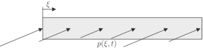
A horizontal line-like structure is exposed to a random stationary 1-direction wind flow with mean ve-locity U (ξ) and a fluctuating gaussian turbulence component u(ξ, t) with standard deviation σ(ξ), see Fig. 1. The wind velocities are assumed to be perfectly correlated in the vertical direction d(ξ) of the line-like structure. Turbulence intensity is defined as Iu(ξ) = σ(ξ)/U (ξ).

Figure 1. A line-like structure immersed in a wind velocity field. The dimensionless curvilinear abscissa is ξ. The covariance between two wind velocities at two positions is defined by

κ2u(ξi, ξj) = σ(ξi)σ(ξj)ρ (sij) (1)

where the correlation function ρ (sij) is assumed to be a function of only the absolute value of the spatial

distance sij =|ξi− ξj| between the two positions. Vertical line-like structures, such as buildings, do not

meet this assumption because the correlation function is also function of the two distinct positions, i.e.

ρ (ξi, ξj, sij).

Assuming quasi-steady aerodynamics, neglecting aerodynamic damping and assuming that the veloc-ity of the structural displacement aligned with the wind is low compared to the wind velocveloc-ity, the total non-gaussian aerodynamic pressure p(ξ, t) on the structure is expressed by

p = a + bu + cu2 (2)

where a(ξ) = γ(ξ)U (ξ)2; b(ξ) = 2γ(ξ)U (ξ); c(ξ) = γ(ξ) with γ(ξ) = 1₂ρ(ξ)d(ξ)C(ξ) where ρ(ξ) is

the air density and C(ξ) is the aerodynamic coefficient. The cross cumulants of order 2 κ2p(ξi, ξj) and

order 3 κ3p(ξi, ξj, ξk) between aerodynamic pressures are respectively given by

κ2pij = bibjρijσiσj+ 2cicjρ 2 ijσi2σj2 (3) and κ3pijk = 2σiσjσk(cibjbkρijρikσi+ bicjbkρijρjkσj+ bibjckρikρjkσk)+8cicjckρijρikρjkσ 2 iσj2σk2. (4)

(2)

Blaise et al. Third order joint acceptance function

2 Background turbulent response

In its continuous form, the background structural response, R(t), is derived from integration of the aerodynamic pressures field p(ξ, t) multiplied by its response-influence function I(ξ) over the line-like structure

R(t) =

∫ 1 0

I(ξ)p(ξ, t)dξ (5)

and its second cumulant is obtained as

κ2R= ∫∫ 1 0 I(ξi)I(ξj)κ2p(|ξi− ξj|)dξidξj ≃ ∫∫ 1 0 g1(ξi)g1(ξj)ρ (|ξi− ξj|) dξidξj (6)

where g1(ξ) = b(ξ)σu(ξ)I(ξ) and neglecting the second term in Eq. (3), which is marginal.

Closed-form expressions of the double integrals in Eq. (6) are attractive in order to avoid numerical integrations and the consideration of numerical admittance (Deno¨el and Maquoi, 2012). This has been achieved by (Dyrbye and Hansen, 1988) who simplified this double integral thanks to the change of variable

sij =|ξi− ξj| and interchange of the order of integration, which finally yields

κ2R= ∫ 1

0

k(s)ρ (s) ds (7)

with an influence function defined as

k(s) = 2

∫ 1−s 0

g1(ξ)g1(ξ + s)dξ. (8)

In the case of integrable expressions for g1(ξ), analytical formulations for the influence function k(s) are derived and even if Eq. (6) has no analytical solution, Eq. (7) has the advantage to reduce the double integration to a single one which is also easier to treat numerically if it had to. Nonetheless, for specific

ρ(s) such as a decaying exponential function

ρ(s) = e−ϕs (9)

with parameter ϕ, analytical solutions of Eq. (7) can be derived. We must also emphasize that analytical expressions for g1(ξ) and ρ(s) may not be available and even with analytical expressions, the double integrals may be awkward (or even impossible) to compute analytically. For simple cases, one may consider fitting those functions with simple polynomial functions which ensures integrability.

The third cumulant of the structural response is obtained as

κ3R =

∫∫∫ 1 0

I(ξi)I(ξj)I(ξk)κ3p(sij, sik) dξidξjdξk

≃ 6

∫∫∫ 1 0

g2(ξi)g1(ξj)g1(ξk)ρ (sij) ρ (sik) dξidξjdξk (10)

where g2(ξ) = c(ξ)σ_u2(ξ)I(ξ) and neglecting the fourth term in Eq. (4), which is marginal. Following the same strategy as discussed hereinbefore, this paper aims at extending the work of (Dyrbye and Hansen, 1988) to a third order analysis, i.e. simplifying triple integrals of Eq. (10) to double integrals as

κ3R = 2 ∫ 1 0 ∫ s1 0 [(k1(s1, s2) + k2(s1, s2))ρ(s1)ρ(s2)] ds2ds1 +2 ∫ 1 0 ∫ 1−s1 0 k3(s1, s2)ρ(s1)ρ(s2)ds2ds1 (11)

(3)

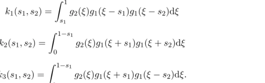
where we define the third order influence functions as

k1(s1, s2) = ∫ 1 s1 g2(ξ)g1(ξ− s1)g1(ξ− s2)dξ (12) k2(s1, s2) = ∫ 1−s1 0 g2(ξ)g1(ξ + s1)g1(ξ + s2)dξ (13) k3(s1, s2) = ∫ 1−s1 s2 g2(ξ)g1(ξ + s1)g1(ξ− s2)dξ. (14)

One could want to apply the same procedure for the fourth cumulant of the structural response, obtained as

κ4R =

∫∫∫∫ 1 0

I(ξi)I(ξj)I(ξk)I(ξl)κ4pijkldξidξjdξkdξl (15) where κ4pijkl is the cross cumulants of order 4 between the aerodynamic pressures. However it comes out that this is quite challenging as interchange of the order of integration is tricky for a four-dimensional domain.

Notice that if analytical expressions are derived for the cumulants of order 2, thanks to Eq. (7), order 3, thanks to Eq. (11), and order 4, thanks to Eq. (15), one could obtain analytical expressions for the skewness coefficient defined as γ3R = κ3R/κ3/2_2R and for the excess coefficient defined as γeR =

κ4R/κ22R. These two coefficients are of paramount importance to assess the non-gaussianity of the structural response and the impact on its extreme values through non-gaussian peak factors (Gurley et al., 1997).

3 Illustration

A beam with constant section and length l is considered. The mean velocity U , standard deviation σu

and coefficient γ are assumed to be constant along the beam. Table 1 collects the influence functions for uniform and linear response influence functions.

Uniform Linear k(s)/(b2σ2) 2(1− s) 1₃(s3− 3s + 2) k1(s1, s2)/ ( b2_cσ4) ₍₁_{− s} 1) ₁₂1 (s1− 1)2 ( s2 1+ 2s1− 2 (s1+ 2) s2+ 3 ) k2(s1, s2)/(b2cσ4) (1− s1) ₁₂1 (s1− 1)2(4s2− s1(s1− 2s2+ 2) + 3) k3(s1, s2)/ ( b2cσ4) (1− s1− s2) −₁₂1 (s1+ s2− 1)2(s1(s1+ 2)− s2(s2+ 2)− 3)

Table 1. Second order and third order influence functions for uniform and linear response influence functions. In the calculation of the cumulants, the correlation function is considered as a decaying exponential function (Holmes, 2007), see Eq. (9). The parameter ϕ = l/Lx_u is the ratio between the length of the structure and Lxu, the integral length scale for the longitudinal turbulence u in direction x(= ξl). The

integral length scale Lx_u is a measurement of the averaged size of the vortices in the wind. In this case, the cross cumulants of order 4 between aerodynamic pressures is given by

κ4pijkl = 4b

2_c2_σ6_(12ρ

ijρikρjl) + 16c4σ8(3ρijρikρjlρkl) (16)

(4)

κ4pijkl ≃ 48b 2_c2_σ6

∫∫∫∫ 1 0

I(ξi)I(ξj)I(ξk)I(ξl)ρ (sij) ρ (sik) ρ (sjl) dξidξjdξkdξl. (17)

Table 2 collects the analytical results for γ3Rand γeRfor uniform and linear response influence functions.

Uniform Linear γ3R 3Iu e−2ϕ(2eϕ_(ϕ+4)+e2ϕ_(4ϕ₋₇₎₋₁₎ 2√2ϕ3(ϕ+e−ϕ−1 ϕ2 )3/2 3√3e−2ϕ(−4eϕ_(ϕ+5)+e2ϕ_(2ϕ(2ϕ_−7)+19)+1₎ 4ϕ4((2ϕ−3)ϕ2+6(ϕ+1) sinh(ϕ)−6(ϕ+1) cosh(ϕ)+6 ϕ4 )3/2 γeR 12I2 u e−3ϕ(eϕ(eϕ(2ϕ(ϕ+9)+2eϕ(8ϕ−19)+47)−2(2ϕ+5))+1)

8(ϕ+e−ϕ−1)2 too long formula.

Table 2. Skewness and excess coefficients for uniform and linear response influence functions.

Figure 1 depicts the cumulants, γ3R and γeR for ϕ ranging [10−3; 102]. Notice for the limit case

of quasi-full correlation, i.e. ϕ ≪ 1; ρ(s) ≃ 1, skewness and excess coefficients approach the values associated to an aerodynamic pressure (resp. 3Iuand 12Iu2) while in the limit case of no correlation, i.e.

ϕ ≫ 1; ρ(s) ≃ 0, their values approach asymptotically the gaussian ones (i.e. zeros) explained by the

central limit theorem (Papoulis, 1965) and the well-known scale effect.

Κ2 RHb2Σu2L Κ3 RH6b2c Σu4L Κ4 RH48 b2c2Σu6L Γ3 RH3IuL Γe,RH12Iu2L 0.1 1 10 100 Φ 0.2 0.4 0.6 0.8 1.0 Uniform: g=1 Κ2 RHb2Σu2L Κ3 RH6b2c Σu4L Κ4 RH48 b2c2Σu6L Γ3 RH3IuL Γe,RH12Iu2L 0.1 1 10 100 Φ 0.2 0.4 0.6 0.8 1.0 Linear: g=x

Figure 2. Cumulants and coefficients as function of ϕ for uniform and linear response influence functions.

References

Deno¨el, V. and Maquoi, R. (2012). The concept of numerical admittance. Archive of Applied Mechanics 82.10-11, pp. 1337–1354.

Dyrbye, C. and Hansen, S. O. (1988). Calculation of joint acceptance function for line-like structures.

Journal of Wind Engineering and Industrial Aerodynamics 31.23, pp. 351–353.

Gurley, K. R., Tognarelli, M. A., and Kareem, A. (1997). Analysis and simulation tools for wind engi-neering. Probabilistic Engineering Mechanics 12.1, pp. 9–31.

Holmes, J. D. (2007). Wind Loading on Structures. 2nd Edition. London: SponPress.