Benchmark of optimization techniques for identification of buildings thermal parameters

HAL Id: cea-01844039

https://hal-cea.archives-ouvertes.fr/cea-01844039

HAL is a multi-disciplinary open access

archive for the deposit and dissemination of sci-entific research documents, whether they are pub-lished or not. The documents may come from teaching and research institutions in France or abroad, or from public or private research centers.

L’archive ouverte pluridisciplinaire HAL, est destinée au dépôt et à la diffusion de documents scientifiques de niveau recherche, publiés ou non, émanant des établissements d’enseignement et de recherche français ou étrangers, des laboratoires publics ou privés.

Houda Zaidi, Sylvain Robert, Frédéric Suard, Yacine Rouis

To cite this version:

Houda Zaidi, Sylvain Robert, Frédéric Suard, Yacine Rouis. Benchmark of optimization techniques for identification of buildings thermal parameters. 14th International Conference of IBPSA - Building Simulation 2015, BS 2015, Dec 2015, Hyderabad, India. pp.2727-2734. �cea-01844039�

BENCHMARK OF OPTIMIZATION TECHNIQUES FOR IDENTIFICATION OF

BUILDINGS THERMAL PARAMETERS

Zaidi Houda

, Robert Sylvain

, Suard Frédéric

, Yacine Ould Rouis

1

CEA LIST, Digiteo Labs Saclay, Bât. 565-PC192, Gif-sur-Yvette, France

ABSTRACT

This article presents an ongoing work aiming at the development of an optimization tool for the assessment of building intrinsic performances. The objective is to enable for the reliable calculation of as-built envelope thermal parameters (resistance and capacitance) based on measurements collected over a limited period of time. The tool is based on the combination of a basic physical model and of optimization algorithms that automatically calibrate the model from measures. This paper presents a benchmarking study lead as part of this work to select an inverse optimization methodology, which is intended to identify a set of thermal parameters. Three methods have been tested for the building thermal inversion. The first method is based on a

simple greedy resolution (Particle Swarm

Optimization) whereas the other two are based on substitution model (Support Vector Regression and Metamodels). The study has been validated on a basic use case (monozonal building) and relied on a comparison between the predictions obtained from calibrated models and those obtained from the Energy Plus simulation environment. The study shows that metamodels coupled with a cross-validation method (kriging) lead to the best results.

INTRODUCTION

Energy is a valuable asset and the basis of

economic growth and societal well-being.

Gradually, energy conservation has become a recognized priority for environment preservation and energy efficiency a prominent concern. The building sector is known to be one of the main contributors to energy consumption. It represents for instance 40% of energy consumption and 36%

of CO2 emissions in the European Union (EU)1.

Therefore, in order to reach the ambitious targets set by recent environmental policies (e.g. the EU

2020 climate and energy package2), energy

performances of buildings have to be significantly improved. In this respect, one major challenge is to enable for reliable and cost-effective assessment of as-built, intrinsic performances. Significant gaps are actually often observed, between “as-designed” and “as-built” building performances (P.De.Wilde 2014). Enabling for the reliable assessment of as-built intrinsic performances would help to identify

1

http://ec.europa.eu/energy/en/topics/energy-efficiency/buildings, accessed April 2014.

2

http://ec.europa.eu/clima/policies/package/index_en.htm,

the causes of possible deviations and, gradually, to tackle their root causes. The good thing is that a significant number of tools for thermal modeling are available. These models are generally gathered into three categories: white box, black box and gray

box models (A. Foucquier 2013a). White box

models describe in details the physical behavior of the system modeled. They include numerous equations, parameters and variables and therefore are usually complex. Black box models, based on statistical models, may provide reliable predictions but do not allow for any physical analysis. Gray box models are hybrid: they rely on simpler physical modeling approaches, but can be calibrated from measures using optimization and statistical learning techniques. They allow for inverse modeling (calculation of actual thermal parameters from measures) with few building information and limited data collection. Gray box models could therefore be a good trade-off between ease of implementation and reliability for the

implementation of intrinsic performances

assessment solutions. However, to unfold their full potential, the following aspects have to be considered with proper attention: (i) the modeling approach shall be simple to use but shall as well allow for the calculation of the main thermal parameters; (ii) the optimization algorithms have both to be reliable and to require reasonable processing time; (iii) the process for collecting the data (building and measurements) shall be swift and simple.

With respect to (i), we presented in a previous paper (A.Foucquier 2013b) a modeling approach based on a thermal-electric analogy that gave a sound foundation to our solution. This paper gives the outcomes of a study lead on the second issue (ii), i.e. the selection and the prototyping of the optimization algorithms.

We specifically focused on the evaluation and testing of three optimization methods: Particle swarm optimization (PSO); the coupling of the PSO method with a regression model based on polynomial support vector regression (SVR); Meta-models validated with a cross-validation method (kriging). The proposed methods are interesting because they can be used both for calibration of a white box model or for the regression of a black box model. In this paper, these methods were used for the calibration of physical model (white box) and in the same time to identify the thermal parameter of single-zonal building. Seven thermal parameters were identified and the predictions from

calibrated were compared to predictions from the EnergyPlus environment.

The paper is structured as follows. A first section introduces the case study and the related model. The subsequent section presents the mathematical foundations of the particle swarm optimization method. The third section illustrates the two substitution models (support vector method and kriging). These two types of models will be compared with a basic theoretical example in the same section and the associated algorithms will be presented. The last section discusses the results obtained on the case study, before giving a conclusion.

CASE

STUDY,

MODEL

PRESENTATION

AND

PROPOSED

SOLUTIONS

In this section, we present the case study. The first sub-section describes the targeted building. Then, the electrical analogy based on Resistance Capacitances (RC)-modeling of the building is described. At last, some considerations about model simplification are given, before highlighting the thermal parameters considered in the optimization phase.

Case study

The geometric information (building, openings) is supposed to be known and is used as an input to the optimization process. We have considered a

mono-zone building of dimension 7.5x6.5x2.5 m3 as

shown in Figure 1. This building includes 7 openings distributed on the 4 façades. Table 1 summarizes the geometrical characteristics of these openings.

Figure 1 Case study geometry

Table 1

Geometric parameters of the openings

D E S IG N A T IO N O F T H E O P E N IN G W1 W2 W3 W4 W5 D1 HEIGHT (M) 2.15 9.5 2.15 1.05 1.05 2.24 WIDTH (M) 2.3 1 1 0.8 0.8 1

RC-network modeling (A. Foucquier 2013a)

The building topology is determined by an undirected weighted graph 𝐺 = (ℵ, ℰ, 𝑊) (K. Deng

2010). ℵ ≔ {1,2, … , 𝑛} denotes the set of nodes of

the graph, ℰ ⊂ ℵ × ℵ denotes the set of edges and

W is the set of edges belonging to the same element

(same wall or zone or opening). A node represents a point measuring temperature and an edge is the segment that connects two adjacent nodes. Each

node 𝑖 ∈ ℵ is assigned by a temperature 𝑇𝑖 and a

capacitance 𝐶𝑖 and each edge 𝑎 = (𝑖 ∈ ℵ, 𝑗 ∈ ℵ) ∈

ℰ is assigned by a resistance 𝑅𝑖,𝑗 that

satisfies 𝑅𝑖,𝑗= 𝑅𝑗,𝑖. Since the thermal model is an

RC-network, its dynamics is described by a system of coupled first order linear differential equations of the form:

𝑪 ⃗⃗ .𝜕 𝑻⃗⃗

𝜕𝑡 (𝑡) = 𝑨 𝑻⃗⃗ (𝑡) + 𝚽⃗⃗⃗ (𝑡) (1)

where 𝑻⃗⃗ (𝑡) = [𝑇1(𝑡), 𝑇2(𝑡), … , 𝑇𝑛(𝑡)]′ denotes the

column temperatures vector at the time t for the set of building nodes mesh, 𝑪 ⃗⃗⃗ = [𝐶1, 𝐶2, … , 𝐶𝑛]′ is the

column vector of nodes capacitance and 𝚽 ⃗⃗⃗⃗ =

[𝜙1, 𝜙2, … , 𝜙𝑛]′ is the column vector of radiative,

solar and net flux. The entries of the transition-rate

matrix 𝑨 = (𝐴𝑖𝑗, 𝑖, 𝑗 ∈ ℵ) are given by:

𝐴𝑖𝑗= { 0 𝑖𝑓 𝑖 ≠ 𝑗 𝑎𝑛𝑑 (𝑖, 𝑗) ∉ ℰ 1 𝑅𝑖𝑗 𝑖𝑓 𝑖 ≠ 𝑗 𝑎𝑛𝑑 (𝑖, 𝑗) ∈ ℰ − ∑ 𝐴𝑖𝑗 𝑗≠𝑖 𝑖𝑓 𝑖 = 𝑗 (2)

The initial temperature is denoted by 𝑇(0).

Model simplification

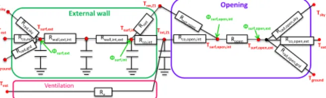
In order to reduce the size of the optimization search space and keep computation time within reasonable boundaries, it is necessary to simplify the geometry. The approach of geometric simplification and its impact on fitness resolution is presented in (A.Foucquier 2013b). This study shows that merging walls and openings has few impact on reliability and improves significantly the performances. Figure 2 shows the model resulting from the application of this simplification approach to our use case. The six walls have been merged into a single wall and the seven openings into a single opening. As can be seen, the wall is supposed a monolayer one and is modeled by a 2R3C (2 resistances, 3 capacitances) configuration.

Figure 2 Simplified RC model of the use case

W1 W2 W4 D1 W5 W3 External wall

Tsurf,ext Tsurf,int Tint,Z1

Rco,ext

Tground

Opening

Rv

Ventilation

Rwall,ext,int Rwall,int,ext Rco,int

Φsurf,ext Φsurf,int Tsky Text Trm,Z1 Text Ropen Rco,open,int Rco,open,ext Tsurf,open,ext Tsurf,open,int Φsurf,open,ext Φsurf,open,int Tground Text Tsky

As a consequence, the number of parameters that will be identified by the optimization algorithms is reduced to 7. These are:

 The overall heat transfer coefficient and

capacitance of the wall (𝑈 =_𝑅𝑆1 , 𝐶), where

R is the wall’s resistance and S is his surface.

 The distribution coefficient of 𝑈 in the

wall (𝐶𝑜𝑒𝑓𝑟𝑒𝑝,𝑈),

 The net flow resistance ℎ𝑛𝑒𝑡 of the wall,

 The overall heat transfer coefficient (U) of

the opening ,

 The radiative distribution coefficient of the

zone (Coefrep,Rad),

 The ventilation rate for the zone

(ACHVentil),

Proposed algorithms presentation

The problem studied does not fit mathematical requirements, it could not be properly solved by classical mathematic and required then a greedy resolution. A grid search resolution is based on building a solution incrementally by adding an item at every step regarding a greedy criterion. In this context a reference method (called particle swarm optimization) was tested for the resolution of our

problem. Despite the simplicity of the

implementation of this method, obtaining optimal solution requires a large number of samples which goes up the run time and do not guarantee that a global minimum of the objective function. Considering that one simulation of a set of parameters needs at least one minute, one have to decrease the number of iterations in order to keep the computation time realistic.

To minimize the number of tests required to obtain the optimal, using a surrogate model can be very interesting. The key of such model is to estimate the overall shape of the cost function in order to guide the convergence procedure. In this context two substitution models have been tested: Support vector machine and kriging models.

The two next sections are devoted to the presentation of the three optimization algorithms. Firstly, we present an optimization tool based on population of random solutions updating for the search of optima. This method is named particles swarm optimization. Secondly, two algorithms based on substitution model are presented. To this end, we first describe the two regression models used (Support vector machine and kriging models). These models are then compared thanks to a basic theoretical test case. At last, the algorithms associated are explained in detail.

GRID SEARCH METHOD:

PARTICULES SWARM OPIMISATION

(PSO)

This is an optimization method developed by Russell Eberhart and James Kennedy (R. Eberhart 1996) which is based on the simulation of the

movement of a particles group. Through

displacement rules of each particle, the particles converge towards an optimal model in the sense of the objective function. This method does not require the calculation of the gradient and therefore can be used for black box models.

Each sample is mapped to a particle. The principle of the PSO method is to use simultaneously multiple particles that explore the solution space by sharing their experience in order to converge to a global minimum. The future position of a particle depends on its velocity and an attraction to the most interesting position met both by each lonely particle and by the group. The PSO algorithm (Y.Cheng 2015) controls the movement of the n particles in space is as follows. At each iteration k, each particle i is defined by:

 Curent position 𝑋𝑖𝑘

 Current velocity Vik

 Best position encountered during travel Pi

 The best position of the set of particles at

the kth iteration Pg.

At each iteration, the velocity of the ith particle is calculated as follows:

𝑉𝑖𝑘+1= 𝜔. 𝑉𝑖𝑘+ 𝑐1. 𝑟𝑎𝑛𝑑. (𝑃𝑖− 𝑋𝑖𝑘)

+ 𝑐2. 𝑟𝑎𝑛𝑑 (𝑃𝑔− 𝑋𝑖𝑘) (3)

Where 𝜔, 𝑐1, 𝑐2 are fixed values, and rand are

random numbers in the [0, 1] interval. The position of each particle is defined by:

𝑋𝑖𝑘+1= 𝑋𝑖𝑘+ 𝑉𝑖𝑘+1 . 𝑑𝑡 (4)

Figure 3 The three steps of the PSO algorithm

Uploading of space work ( best> convand iteration number < iteration number max)

As convergence is wrong : For each particle:

* Change the velocity of the particle and the new particule

* Evaluate the finesse of this new particle ( i,new) and

update the best population and the best particule

Initializing

- Simulate the images of these samples (Y1, ..., YN)

- Evaluate the fitness of each particle ( 1 ... N)

- Fix the best population best = (P1, ..., PN) and the best

particule (Pbest, best)

Starting space

- Set a starting set = (P1, ..., PN) and

The movement of the group of particles is evaluated until the algorithm converges or until the maximum number of iterations is reached. Figure 3 outlines the three steps of the algorithm.

METHODS BASED ON

SUBSTITUTION MODEL

In an optimization process, using a simple analytical and differentiable model is preferable. Substitution models have the advantage to give a good approximation of the system response, in a simpler and more manageable way. Such models can be a simple mathematical representation of a numerical model, a black box model, or a behavioral model (related to experimental data). There are a variety of mathematical models classified under this category. These methods are commonly used for the benefits they provide:

 An understanding of the relationship

between the governing inputs and outputs of the model

 A quick analysis tool for optimization

 A quick and easy coupling between

dependent fields and disciplines.

This approximation via mathematical models

involves three requirements classified and

characterized in (T. Simpson 2001)

 The choice of experiments points,

 The choice of the type of model best suited

to the representation of data,

 The experiments approximation (fitting),

i.e. the determination of the unknown parameters of the model equations. In this study, two algorithms based on substitution model have been used: SVR and kriging metamodel.

Substitution models

Support vector method (SVM)

Support vector machines (SVMs) are a set of related supervised learning methods that analyze data and recognize patterns, used for classification (machine learning) and regression analysis. The original SVM algorithm was invented by Vladimir Vapnik (V.Vapnik 1995).

Suppose a set of observational data (samples) (𝑋1, 𝑌1), (𝑋2, 𝑌2), . . . , (𝑋𝑘, 𝑌𝑘) such as 𝑋𝑖∈ ℝ𝑛 and

associated value 𝑌𝑖∈ ℝ ∀ 𝑖 ∈ {1, … , 𝑘} . For the

regression problem based on the SVM, the objective is to find a function 𝑓 that minimizes the

difference between 𝑓(𝑋𝑖) and 𝑌𝑖, ∀ 𝑖 ∈ {1, … , 𝑘}.

The function that was used in this work is polynomial of order 2 and the quadratic optimization problem was solved with the interior point method. This function is named the SVM regression function and can be written as:

𝑓(𝑋) = ∑ 𝑤𝑖𝐾(𝑋, 𝑋𝑖)

1≤𝑖≤𝑛

+ 𝑏 ₍₅₎

where K is a 2-order polynomial kernel function

𝐾(𝑋, 𝑋𝑖) = (〈𝑋, 𝑋𝑖〉 + 1)2 (6)

Kriging metamodel

Kriging is an approximation or modeling method based on a statistical model (J. Sacks 1989). The typical use of this approximation is to construct a prediction model based on experimental data.

Given a set of m samples S = [X1, … , XM] with

Xi ∈ ℝn and the answers Y = [Y1, … , YM] with

Yi∈ ℝ. The data are assumed to satisfy the

normalization conditions:

{μ[S(: , j)] = 0, V[S(: , j), S(: , j)] = 1, j = 1, … , n μ[Y] = 0, V[Y, Y] = 1, (7)

μ, V denote the mean and covariance respectively.

We assume a model ŷ which approximates the

response y (x) ∈ ℝ, for an n-dimensional input

x ∈ D ⊂ ℝn_{, based on a regression model ℱ and a}

random function (stochastic process) z such as :

ŷ (x) = ℱ(β, x) + z(x) (8)

Validation and comparison of the substitution models

This paragraph illustrates the validation of the two substitution model thanks to a simplified, theoretical use case. The aim is to compare the resulting model obtained with SVR and kriging with a theoretical model that has been analytically defined.

Validation case:

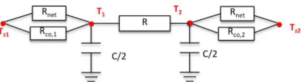
We studied an RC model consisting of two nodes to represent the behavior of a homogeneous single

layer wall that separates two adjacent areas z1 and

z2 (Figure 4).

Figure 4 modelling of heat transfer between two zone by a 1R2C network wall

This network can be translated to the following system of equations: R Rco,1 R_net Rco,2 T1 T2 Tz2 Tz1 Rnet C/2 C/2

(𝐶/2 𝐶/2) ( 𝜕𝑇1 𝜕𝑡 𝜕𝑇2 𝜕𝑡 ) = ( −1 𝑅− 1 𝑅𝑐𝑜,1− 1 𝑅𝑛𝑒𝑡 1 𝑅 1 𝑅 − 1 𝑅− 1 𝑅𝑐𝑜,2− 1 𝑅𝑛𝑒𝑡₎ ⏟ 𝐴(𝑅,𝐶) (𝑇1 𝑇2 ) + ( 1 𝑅𝑐𝑜,1+ 1 𝑅𝑛𝑒𝑡 0 0 1 𝑅𝑐𝑜,2+ 1 𝑅𝑛𝑒𝑡₎ ⏟ 𝐵(𝑅,𝐶) (𝑇𝑧1 𝑇𝑧2) (9) With:

 Tz1, Tz2: Temperature of the two adjacent

zone z1 and z2 [°C]

 T1, T2: Temperature of the two surfaces of

the wall [°C]

 S : Surface of the wall [m2]  R: Resistance of the wall [K/W]

 C: Heat capacity of the wall [J/K]

 Rco,1, Rco,2 : the two convection resistances

of the wall [W/(m2.K)]

 Rnet: net resistance of the wall

The parameters to be determined are the thermal resistance R of the wall, and its heat capacity C. The other variables are either measured or pre-determined. We consider the wall that separates the ground floor and the subsoil in the I-MA house of the INCAS experimental platform of the French National Institute of Solar Energy (INES) in Le-Bourget-du-Lac. The values of the other parameters describing the wall are (Clara 2012):

 Rco,1 = 0.01 W/(m2.K)

 Rco,2 = 0.0045 W/(m2.K)

 Rnet = 0.004 W/(m2.K)

We use the SVR and the kriging models to

construct a polynomial function 𝑦̂𝑝 that predicts the

behavior of: 𝐹(𝑅, 𝐶) = ‖(𝐶/2 𝐶/2) ( 𝜕𝑇1 𝜕𝑡 𝜕𝑇2 𝜕𝑡 ) − 𝐴(𝑅, 𝐶). (𝑇1 𝑇2 ) − 𝐵(𝑅, 𝐶). (𝑇𝑧1 𝑇𝑧2)‖ (10)

The search space is defined by the “typical”

intervals of values 𝑅 ∈[0.1; 50]K/W and

𝐶 ∈ [1; 1𝐸8](𝐽/𝑊). Results and comparison

For the validation of the two substitution model studied in this paper, we used these models to estimate the function F. The estimation of this

function is performed according to an order 2 polynomial. The construction of the SVR models requires three experimental points by again the kriging model need six experimental points. To compare the two models, six samples points (set of evaluations function use to construct the models) are considered for the construction of the SVR and kriging model. The Figure 5 shows the approximation of the function test F by the kriging and SVR models for distribution of the six samples points. The error average quadratic (MSE (6)) is illustrated in Figure 6 for the two models (J. Sacks 1989).

𝑀𝑆𝐸 = 𝜎2_{[1 − 𝑟}𝑇_𝑅−1_{𝑟 +}(1 − 1𝑇𝑅−1𝑟)2

1𝑇_𝑅−1₁ (11)

With :

 R : the correlation matrix between the

different samples points,

 r : the vector which represents the

correction between the n samples points and unevaluated variable

Figure 5 SVR and kriging polynomial model with 6 samples data

Figure 6 Mean squared error of the SVR and kriging polynomial model

We note that the average error between the model and the function is very low in the vicinity of the samples points. Furthermore, the error increases on the ends of the domain. In the cases treated, the

SVR model could reproduce a faithful

approximation of the function only on the vicinity of the samples points. In addition, an increase in the number of these sample points will significantly

improve the modeling results. The same

observation can be made with the kriging model but

2 3 4 2 4 6 C[J/K]*1E6 R[W/(m².K) SVR model Samples data Funcion F(R,C) 2 2.5 3 3.5 4 0 2 4 6 C[J/K]*1E6 R[W/(m².K) Kriging model Samples data Function F(R,C) 2 3 4 2 4 6 0 0.02 0.04 0.06 0.08 0.1 0.12 C[J/K]*1E6 R[W/(m².K) M S E S V R m od el 2 3 4 2 4 6 0 0.02 0.04 0.06 0.08 0.1 C[J/K]*1E6 R[W/(m².K) M S E K ig in g m o d el 0 0.02 0.04 0.06 0.08 0.1 0.12 0.02 0.04 0.06 0.08 0.1

the error is lower than the one obtained with the SVR model.

Algorithm based on SVR model

Since the two models seem to be able to fit the targeted function that implies thermal parameters the global procedure of parameters estimation could be described.

The algorithm starts by choosing n random samples

(𝑋1, … , 𝑋𝑁) and then simulates these samples with

our model (𝑌1, … , 𝑌𝑁), so that the difference with

the reference temperature(𝜉1 = |𝑌1− 𝑌𝑅|, … , 𝜉𝑁=

|𝑌𝑁− 𝑌𝑅| is minimized. SVM is then used to

determine a regression model denoted 𝑓 such as

𝑓(𝑋𝑖) ≈ 𝜉𝑖. To validate this model, the following

fitness function is used:

𝑓𝑖𝑡𝑛𝑒𝑠𝑠 =_𝑁1∑1≤𝑖≤𝑁|𝑓(𝑋𝑖) − 𝜉𝑖|.

Once the SVM regression model is validated, the PSO method is used to determine the minimum

(𝜉𝑆𝑉𝑅,𝑚𝑖𝑛) of the SVR function f that matches to the

set of parameters 𝑋𝑚𝑖𝑛,𝑓 (𝜉𝑆𝑉𝑅,𝑚𝑖𝑛= 𝑓(𝑋𝑚𝑖𝑛,𝑓).

The algorithm is stopped if the 𝜉𝑆𝑉𝑅,𝑚𝑖𝑛 reaches the

convergence criterion. Otherwise 𝑋𝑚𝑖𝑛,𝑓 and other

new particles are added to the set of samples.

Figure 7 summarizes the successive steps of the

SVR-PSO algorithm.

Figure 7 PSO-SVM algorithm Algorithm based on kriging model

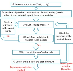
The algorithm starts with the selection of an initial set of samples and the simulation of all samples possible combinations (step 1 and 2); this leads to the construction of an observation data space (samples) (𝑋1, 𝑌1), (𝑋2, 𝑌2), . . . , (𝑋𝑟, 𝑌𝑟) such as

𝑋𝑖∈ ℝ𝑛 and 𝑌𝑖∈ ℝ ∀ 𝑖 ∈ {1, … , 𝑟}. The next step

is to adjust r kriging metamodels for these simulation data (step 3) and validate these models (step 4). As the test proclaims one or more invalid meta-models, we update the design of models by simulating of additional input combination (step 5)

of global research area in order to further refine the r- metamodels.

When all r kriging models are valid, a solver is used to estimate the optimal location based on the kriging model (step 6). Then the algorithm checks whether the optimal sample has already been simulated and if the convergence criterion is reached (step 7). In the case where the convergence criteria have not yet been reached, another combination is added to the previous base (step 8). The algorithm is summarized in Figure 8 (J.P.C. Kleijnen 2010), (J.P.C.Kleijnen 2014).

Figure 8 Kriging algorithm

RESULTS AND COMPARISON

The three methods previously described and validated on the theoretical case have been applied to the mono-zone building use case. The aim is to calculate the values of the seven thermal parameters listed in the previous section. The following figure shows the evolution of the error as a function of the number of iterations, for each the three methods until the convergence is obtained.

The results show the limitation of PSO method, where the convergence process is slow due to the attraction of local minima with 100 iterations whereas SVR or kriging obtain a similar error with only 30 iterations. Since each iteration requires a significant processing time, this approach does not seem to be well suited for our application scope. On the contrary, PSO-SVR and kriging give better results. They are able to significantly reduce the number of iterations and thus the calculation time. Kriging seems to bring an additional benefit from the robustness point of view: the algorithm is less sensitive to local minima and results in a smoother convergence pattern. The number of models evaluations required to reach the optimal solution is past from 500 with the PSO method to 250 with PSO-SVR method and 150 with kriging method. Set a starting set Ƥ=(P1, …, PN),

simulate the images of these samples (Y1, …, YN) (1),

Evaluate the fitness of each particle (ζ1, …ζN) (2)

SVR learning (build a SVR model such as (SVR(Pi)≈ ζi) (3)

Validate the model (max(|SVR(Pi)-ζi|)) Non-validated model Introduce new particles

Research the minimum of this model with PSO and calculate the fitness of this minimum

Introduce new particles

Convergence validat model

 Consider a starter set Ƥ=(P1, …, PN),

 Simulate all possible combinassions of this assembly (need a number of replication)  r particle are thus available

Adjust r kriging model (*)

Apply Cross validation to validate these models No

Yes

Find the minimum of each model  Detect and simulate the best minimum  Add a point near to the worst points Convergence criterion checked Convergence criterion Unaudited Add the minimum or the next minimum

This significant reduction is reflected in a significant reduction in calculation time (4h for PSO method, 2h for PSO-SVR method and 1.5h for kriging method). The number of models evaluation is different from the iteration number because the three algorithm start with a no-single set of samples. Moreover, the PSO algorithm reevaluates the start set sample at each iteration, which explains the considerable increase of the evaluation models total number.

Figure 9 Application of the optimization methods to the use case. Evolution of the error as a function of the number of iteration.

The validation of our model is performed over a period of one year. However, for the clarification of the result visualization, only two weeks are represented. Indeed, Figure 10 indicates the operative temperature over two weeks for the results obtain with the three proposed optimization algorithms compared with the EnergyPlus result. As we can see, the temperature estimated with the kriging model is much more representative of the reference temperature of EnergyPlus.

Figure 10 Operative temperature comparaison of the optimization and EnergyPlus results for the quasi-passive monozonal building

The evolution of the error between the operative temperature and the EnergyPlus simulation results displayed in Figure 11 for the three algorithms. The error distribution around the average value is showed in the Figure 12.

Figure 11 Histograms of the error between the operative temperature and EnergyPlus results for the quasi-passive monozonal building

Figure 12 Distribution of the error for the 3 proposed optimisation algorithms

The three histograms show a Gaussian error distribution. The mean of the error distribution µ is equal to the value of convergence criterion of the

algorithms. The standard deviation 𝜎 of the error

distribution is significantly larger with the PSO algorithm compared to the two other algorithms where the standard derivation is almost identical (see Figure 13, where the values of the parameters identified obtained with the three algorithms is displayed).

Figure 13 Numeric values of the parameters identified with the three algorithms optimization

The results presented above indicate a small error (≤ 5%) between the parameters identified with the three algorithms. We can then use these algorithms not only for, the calibration of our physical model but also the estimation of building intrinsic performances. 0 50 100 150 200 0.2 0.4 0.6 0.8 1 1.2 1.4 1.6 Iteration number E rr o r PSO model Kriging model SVR model 5 10 15 20 25 30 35 40 0.2 0.4 0.6 0.8 1 1.2 1.4 Iteration number E rr o r SVR model Kriging model PSO model 01/02/12 03/02/12 05/02/12 07/02/12 09/02/12 11/02/12 13/02/12 15/02/12 0 5 10 15 T em p er at u re i n ° C 01/02/12 03/02/12 05/02/12 07/02/12 09/02/12 11/02/12 13/02/12 15/02/12 0 5 10 15 Time T em p er at u re i n ° C 03/02/12 05/02/12 07/02/12 09/02/12 11/02/12 13/02/12 15/02/12 17/02/12 0 5 10 15 T em p er at u re i n ° C

Temperature wih PSO inversion EnergyPlus Temperature

EnergyPlus Temperature Temperature wih PSO-SVR inversion

Temperature wih kriging inversion EnergyPlus Temperature -2 -1.5 -1 -0.5 0 0.5 1 1.5 2 0 2000 4000 6000

Histogram of the error for the PSO algorithm

-2 -1.5 -1 -0.5 0 0.5 1 1.5 2

0 2000 4000 6000

Histogram of the error for the PSO-SVR algorithm

-2 -1.5 -1 -0.5 0 0.5 1 1.5 2

0 2000 4000 6000

Histogram of the error for the Kriging algorithm

-3 -2 -1 0 1 2 PSO PSO-SVR Kriging MIN 25% 50% 75% MAX 0 10 20 30 40 50 PSO algorithm Krigin algorithm PSO-SVR algorihm ACH Ventil Coef rep,Rad U open h net Coef_rep,U C*1e-6 [J/K] R [K/W]

CONCLUSION

Energy efficiency is a prominent concern in the AEC sector. Modeling and simulation tools can help to reduce the energy consumption of the building and meet the requirements of existing energy labels, but fail to solve the “energy gap”

problem – deviation of as-built energy

performances from as-designed performances. It would therefore be beneficial to generalize as-built intrinsic performances assessment tools, able to reliably calculate the actual performances from limited (in time and scope) measurements. One promising path, to enable such tools, is to rely on so-called “grey-box” modeling approaches, which advocate the combination of simplified physical models and optimization algorithms. These approaches allow for the calibration of the models from measurements and, this way, for the deduction of the thermal parameters of the building, i.e. inverse modeling of the building.

This paper gave an account of as study lead as part of the development of such an inverse modeling tool. The first steps of this development focused on the definition of a simplified modeling approach (A. Foucquier 2013a) and (A.Foucquier 2013b). The study described in this paper focused on the assessment and selection of the optimization algorithm. Three optimization methods were implemented and compared (PSO, PSO-SVM, and kriging), based on a simple mono-zone building use case. The results show that convergence is faster in the case of PSO-SVM and kriging. PSO alone tends to get attracted by local minima and does not perform as well. The convergence patterns also suggest that kriging will be more robust and probably, the best candidate.

ACKNOWLEDGEMENTS

The work presented in this paper was supported by the European Community's Seventh Framework Programme under Grant Agreement no.609154 (Project PERFORMER). We are also grateful to Dr. Hassan Sleiman from CEA LIST for his revisions and comments, as well as Florent Alzetto from Saint Gobain, Rémi Bouchié from CSTB and Adrien Brun from CEA LITEN for their fruitful feedback on this research.

REFERENCES

A. Foucquier, S. Robert, F. Suard, L. Stéphan and A. Jay. «State of the art in building modelling andd energy performances prediction : a review.» Renewable and

Sustainable Energy Reviews, 2013a:

272-288.

A.Foucquier, A.Brun, GA.Faggianelli and F.Suard. "Effet of wall merging on a simplified building energy model : accuracy vs

number of equations." Proceedings of

IBPSA, 2013b: 3161-3168.

Clara, S. «Analysis of simulation tools reliability and measurement uncertainties for Energy Efiiciency in Buildings.» Phd thesis, 2012. D. Tuia, J. Verrelst, L.Alonso, F.Perez-Cruz and G.

Camps-Valls. «Multioutput Support

Vector Regression for Remote Sensing

Biophysical Parameter Estimation.»

Geoscience and Remote Sensing Letters, IEEE, 2011: 804-808.

J. Sacks, W. J. Welch, T. J. Mitchell and H. P. Wynn. «Design and Analysis of Computer Experiments.» Statistical Science, 1989: 409–423.

J.P.C. Kleijnen, W.V. Beers and I.V.

Nieuwenhuyse. «Constrained optimization in expensive simulation: Novel approach.»

European Journal of Operational

Research, 2010: 164-174.

J.P.C.Kleijnen. «Simulation-optimization via

Kriging and bootstrapping: a survey.»

Journal of Simulation, 2014: 241-250.

K. Deng, P. Barooah, P.G. Mehta and S.P. Meyn. «Building thermal model reduction via aggregation of states.» American Control

Conference (ACC), 2010: 5118-5123.

P.De.Wilde. «The gap between predicted and mesured energy performance of buildings : a framework for investigation.» Automatic

in construcion, 2014: 40-49.

R. Eberhart, P. Simpson and R. Dobbins.

Computational intelligence PC tools.

Academic Press Professional, Inc., 1996. S.Yin, H.B.Zhao and. «Geomechanical parameters

identification by particle swarm

optimization and support vector machine.»

Applied Mathematical Modelling, 2009:

3997 - 4012.

T. Simpson, J. Poplinski, P. N. Koch, and J. Allen.

«Metamodels for computer-based

engineering design : Survey and

recommendations.» Engineering with

Computers, 2001: 129–150.

V.Vapnik, C.Cortes and. Support-Vector Networks.

Kluwer Academic Publishers-Plenum

Publishers, 1995.

Y.Cheng, R.Jin and. «A social learning particle swarm optimization algorithm for scalable optimization.» Information Sciences, 2015: 43-60.