Influence des fluctuations climatiques sur la xylogénèse de Picea mariana des sites mésiques de la forêt boréale continue

UNIVERSITE DU QUEBEC A CHICOUTIMI

INFLUENCE DES FLUCTUATIONS CLIMATIQUES SUR LA XYLOGENESE DE

PICEA MARIANA DES SITES MÉSIQUES DE LA FORÊT BORÉALE CONTINUE

PAR BORIS DUFOUR B. SC. (BIOLOGIE)

M. SC. (RESSOURCES RENOUVELABLES)

THESE PRESENTEE

À L'UNIVERSITÉ DU QUÉBEC À CHICOUTIMI COMME EXIGENCE PARTIELLE

DU DOCTORAT EN SCIENCES DE L'ENVIRONNEMENT

TABLE DES MATIÈRES

Table des matières ii Liste des tableaux et figures v Avant-propos viii 1. Introduction 1 1.1 Mise en contexte ...1 1.2 Cadre de l'étude 3 1.3 Objectifs généraux 5 1.4 Hypothèses générales 5 1.5 Méthodes d'échantillonnage 7 1.6 Méthodes d'analyse 8 1.7 Organisation de la thèse 10 2. Focusing modelling on the tracheid development period - an alternative method for treatment of xylogenesis intra-annual data 11

2.1 Summary 11 2.2 Introduction 13 2.3 Materials and methods 15 2.3.1 Study areas 15 2.3.2 Sampling 15 2.3.3 Sample processing and xylogenesis data collection 16 2.3.4 Standardization 16 2.3.5 Restricting the datasets 17 2.3.6 Defining the total number of cells 17 2.3.7 Regression 18 2.3.8 Comparison between weekly and semi-monthly sampling 19 2.4 Results and discussion 19 2.4.1 Restricting the datasets 19 2.4.2 Fitting a function 21 2.4.3 Comparison between weekly and semi-monthly sampling 23 2.5 Conclusion 26 2.6 Acknowledgement 27 2.7 References 28 3. Tracheid production phenology of Picea mariana and its relationship with climatic fluctuations and bud development using multivariate analysis 31

3.1 Summary 31 3.2 Introduction 33 3.3 Materials and methods 35

3.3.1 Study area and sampling plots 35 3.3.2 Assessment of in-progress cell production 36 3.3.3 Assessment of bud break 38 3.3.4 Meteorological monitoring and climatic variability 38 3.3.5 Modeling method 40 3.3.6 Regressors compilation and response variables transformation 43 3.3.7 Comparing the influence of each important factor 44 3.4 Results 44 3.4.1 Timing of tracheid production and bud break 44 3.4.2 Influence of climatic variations on timing of tracheid production initiation 46 3.4.3 Influence of climatic variations on timing of tracheid production cessation 49 3.5 Discussion 52 3.5.1 Modeling methods 52 3.5.2 Timing of tracheid production 52 3.5.3 Tracheid production initiation: link with bud initiation and climate 53 3.5.4 Influence of climatic variations on timing of tracheid production cessation 55 3.5.5 Predictive utility 57 3.5.6 Black spruce tracheid production season vs climate changes 58 3.6 Conclusion 58 3.7 Acknowledgement 59 3.8 References 59 4. Phenology-linked multifactorial analysis of tracheid production in the trunk of Picea

mariana 67

4.1 Summary 67 4.2 Introduction 69 4.3 Materials and methods 71 4.3.1 Study area and sampling plots 71 4.3.2 Assessment of tracheid production phenology 72 4.3.3 Total annual tracheid count and measurements 73 4.3.4 Meteorological monitoring and climate variability 74 4.3.5 Modeling radial increment 76 4.3.6 Modeling the seasonal tracheid production 77 4.3.7 Weighting the contribution of variables 79 4.4 Results 80 4.4.1 Number of tracheids produced and its importance for cell width 80 4.4.2 Influence of climate on black spruce tracheid production 82 4.5 Discussion 84 4.6 Conclusion 89 4.7 Acknowledgements 90 4.8 References 91

5.2 Introduction 100 5.3 Materials and methods 101 5.3.1 Study area and sampling plots 101 5.3.2 Assessment of tracheid radial development phenology 102 5.3.3. Total annual tracheid count, dimensions and standardization 102 5.3.4 Modeling the tracheid diameter transition throughout the ring 103 5.3.5 Meteorological monitoring and climate variability 104 5.3.6 Linking tracheid diameter with climate data using tracheid development

phenology 106 5.3.7 Modeling method 107 5.4 Results 108 5.4.1 Tracheid diameter transition 108 5.4.2 Environmental influence on tracheid diameter 112 5.5 Discussion 114 5.5.1 Tracheid diameter transition 114 5.5.2 Factors influencing tracheid diameter in the first period 117 5.5.3 Factors influencing tracheid diameter in the second period 118 5.6 Conclusion 119 5.7 Acknowledgement 120 5.8 References 121 6. Conclusion générale 125 6.1 La dynamique d'accroissement radiale chez l'épinette noire 125 6.2 Influence des facteurs climatiques 126 6.2.1 Luminosité 126 6.2.2 Température de l'air 127 6.2.3 Température du sol 129 6.2.4 Humidité de l'air 130 6.2.5 Disponibilité en eau 130 6.3 Théorie émergente: un cerne de croissance qui dépend de la taille des bourgeons et des conditions propices à la photosynthèse concomitante à sa formation 131 6.4 Perspectives 134 6.4.1 Une étude innovante 134 6.4.2 Les limites et les implications de l'étude 135 7. Références des chapitres 1 et 6 139

LISTE DES TABLEAUX ET FIGURES

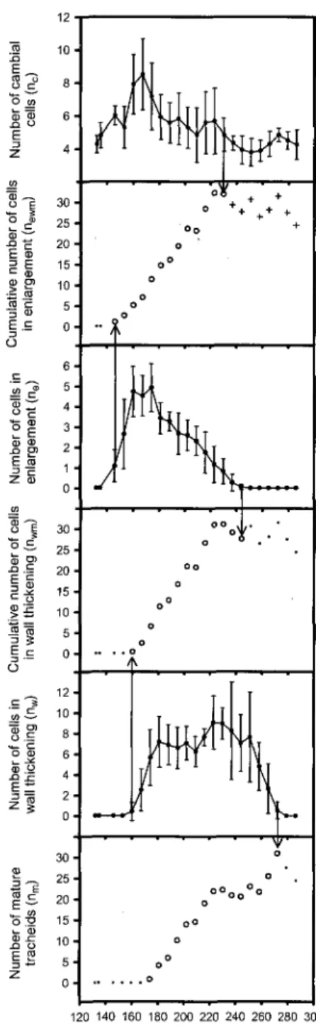
Figure 2.1. Example showing the selection process for the observations of newm, nwm and

nm that are to be regressed (open circle markers). Plain circle markers for n<;, ne and nw

represent observations along with their respective standard deviation (vertical bars). Large open circle markers for newm, nwm and nm represent observations selected as part of the

active period of each dataset, and small plain circle markers represent the unselected ones. Cross-shaped markers are unselected observations for neWm indicating an achieved Ctot and

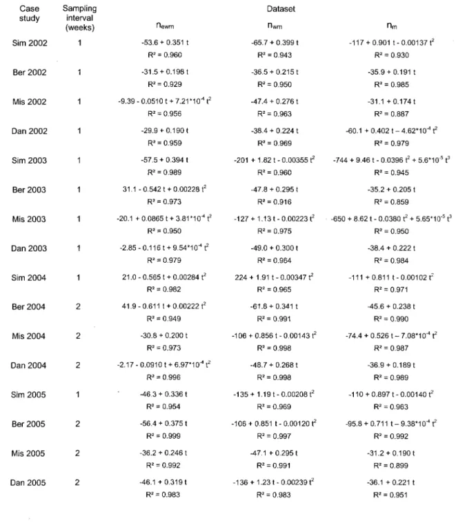
serving for the evaluation of this parameter 20 Table 2.1: Fitted functions (t is time in Julian days), adjusted R2 and sampling interval

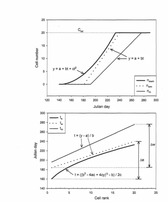
length for the different cases studied 22 Figure 2.2. Example of the resulting functions for one case study (Ber 2004) in the fitted (neWm, nwm and nm) and the inversed (te, tw and tm) forms. Functions are developed only

along the functional range of the case study, which is delimited by 0 and Ctot. General

equations are given for each function type (1st and 2nd degree polynomials) and the overall

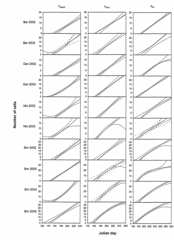
phases range are illustrated (Ae) and (Aw). In the functions, y is the cell number and t is the time and a, b and c are function parameters 24 Figure 2.3. Comparison between fitted function for simulated semi-monthly sampled

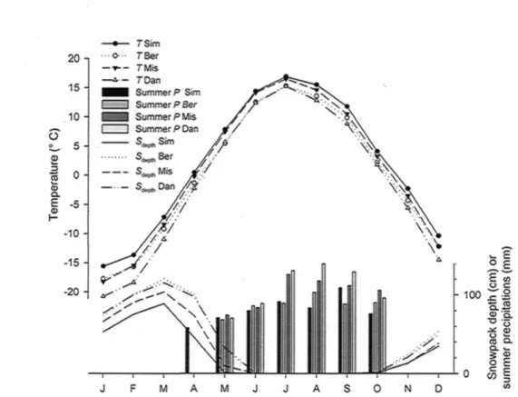
dataset (plain lines) and the corresponding confidence interval (95 %) fitted on weekly sampled dataset (dashed lines). When inclusion is not in the whole range, confidence interval for the semi-monthly fitting is also shown (dotted lines) to check for overlapping with the one for the weekly fitting 25 Figure 3.1. Monthly mean Temperature (7), total precipitations of months with mean temperature over 0 °C (Summer P), and mean snowpack depth (5depth) from 2002 to 2006

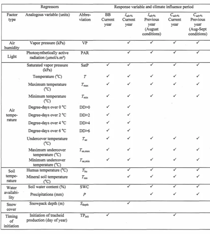
for each site 40 Table 3.1. Check list of candidate regressors tested for their influence on various

phenological response variables of different nature and period of influence. Regressors are all means computed from daily data and covering periods specific to each model. Response variables abbreviation: BB, bud break; /adv%, daily percentage of advancement to tracheid

production initiation; Caciv%, daily percentage of advancement to cessation of tracheid

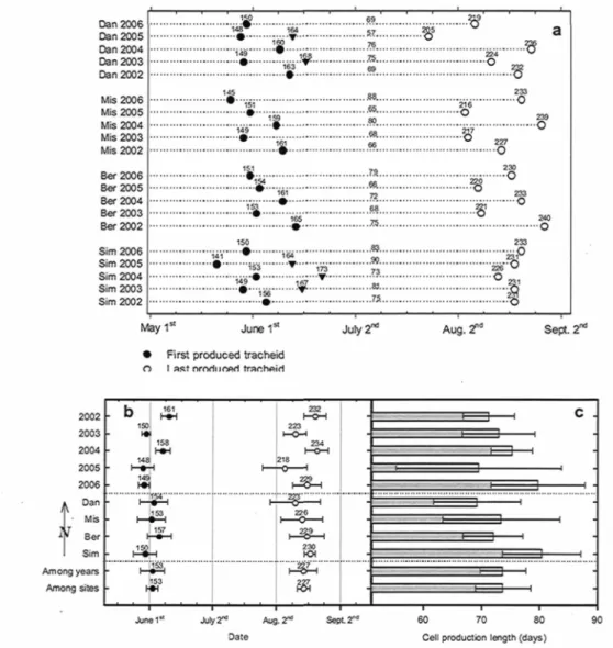
production 42 Figure 3.2. Timing of cambial and apical phenology (a) giving: tracheid production

initiation, tracheid production cessation, bud break, all three with symbols tagged on day of year. Duration of tracheid production is also given by tags above dotted lines. Cambial initiation and cessation have been compiled for every year (mean of 4 sites), every site (mean of 5 years) and then re-averaged for overall variation across years and sites (b), and

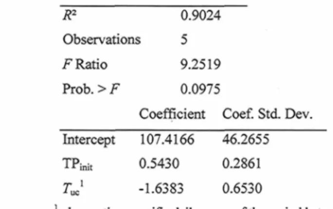
Table 3.2. Multiple regression ANOVA and model coefficients of the multiple regression computed for bud break timing vs. timing of tracheid production initiation (TPimt) and

undercover temperature (Tuc ) 46

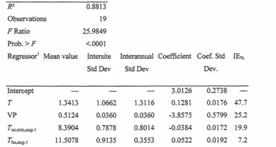
Table 3.3. Multiple regression ANOVA, climatic variables' mean and standard deviations, model coefficients and their standard deviation, and percentage of independent effect (IE%) given by hierarchical partitioning of the best multiple regression found for daily percentage of advancement to tracheid production initiation (/adv%) vs. daily climatic variables 47

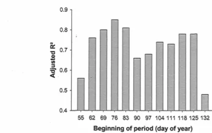
Figure 3.3. Adjusted R2 for 12 iterations of the modeling process (see methods) for daily

percentage of advancement to tracheid production initiation (/adv%) in function of climatic

variables. In each iteration (bar), the length of the considered period for climate influence is changed by modifying its beginning day, in such a way for climate and response

variables to be differentially compiled for each of these periods. All models are significant (a = 0.05) 48 Figure 3.4. Daily probability for daily mean temperatures (T) over 0 °C to occur. These have been calculated by dividing the number of observed occurrence of T > 0 over all observed cases (20), on the four sites from 2002 to 2006. The arrow points to the starting day of the best fit period of climate influence as previously determined (day 76) 49 Figure 3.5. Adjusted R2 for 16 iterations of the modeling process (see methods) for daily

percentage of advancement to tracheid production cessation (Cadv%) in function of climatic

variables. In each iteration (bar), the length of the considered period for climate influence is changed by modifying its beginning day, in such a way for climate and response

variables to be differentially compiled for each of these periods. All models are significant (a = 0.05) 50 Table 3.4. Multiple regression ANOVA, climatic variables' mean and standard deviations, model coefficients and their standard deviation, and percentage of independent effect (IE%) given by hierarchical partitioning of the best multiple regression found for daily percentage of advancement to tracheid production cessation (Cadv%) vs. daily climatic variables 51

Table 4.1. Checklist of candidate regressors of different type and operational period; these have been tested for their influence on the number of tracheids produced. Regressors are all means computed from daily data. TP refers to tracheid production period 79 Figure 4.2. Number of tracheids produced at the four studied sites from 2002 to 2006 81 Table 4.2. Paired-by-site correlations of the number of tracheids produced from 2002 to 2006, along with their significance probability (P) 82 Table 4.3. Multiple regression ANOVA, model coefficients and their standard deviation, and percentage of independent effect (IEo/o) given by hierarchical partitioning of the best

multiple regression found for the number of tracheids produced vs. duration and climate variables selected in a first run. Mean value is also indicated 83 Table 4.4. Cross correlations of the variables selected in the multivariate model and the number of tracheids. A single asterisk indicates a significant correlation (a = 0.05) while a double asterisk indicates a highly significant correlation (a=0.01) 83 Figure 4.3. Student comparison of the mean number of tracheids produced at each site without taking climate into account (top) and once the effect of climate is removed

(bottom) 84 Table 4.5. Description of four newly tested variables. Any of them are selected when

confronted to the four variables of the model shown in this paper 88 Figure 5.1. Monthly mean temperature (7), total precipitations of months with mean

temperature above 0 °C (Summer P), and mean snowpack depth (Sdepth) from 2002 to 2006 for each site 105 Figure 5.2. Measured (dots) and modeled (lines) tracheid diameter along tree ring radial direction from the first (pith side) to the last (bark side) tracheid 109 Figure 5.3. a: Timing of the tracheid diameter breakpoint for the 20 combinations of site and year, b: Timing compiled by year, c: Timing compiled by site. Error bars are standard deviation 110 Table 5.1. Multiple regression ANOVA, model coefficients and standard deviation, as well as percentage of independent effect (IE%) given by hierarchical partitioning of the best multiple regression found for the timing of tracheid diameter breakpoint vs. climate during the period between tracheid production initiation and the breakpoint. All candidate

regressors tested are listed, but only those parts of the selected model have parameters displayed I l l Table 5.2. Multiple regression ANOVA, model coefficients and standard deviation, as well as percentage of independent effect (IE%) given by hierarchical partitioning of the best multiple regression found for tracheid diameter before the tracheid diameter breakpoint vs. climate during cell enlargement. All candidate regressors tested are listed, but only those parts of the selected model have parameters displayed 113 Table 5.3. Multiple regression ANOVA, model coefficients and standard deviation, as well as percentage of independent effect (IE%) given by hierarchical partitioning of the best multiple regression found for tracheid diameter vs. climate during cell enlargement after the tracheid diameter breakpoint 114

AVANT-PROPOS

Le projet de thèse original a été déposé il y a 10 ans. À cette époque, les professeurs Hubert Morin et Réjean Gagnon de l'UQAC avaient obtenus des fonds pour l'installation de quatre stations météo permettant de mesurer le climat sur quatre stations d'échantillonnage, non établie. Je fus donc engagé à l'automne 1999 et à l'été 2000, préalablement à mon inscription au doctorat, afin de faire la recherche de sites propices à l'établissement de ces quatre stations, ainsi que pour préparer le terrain et y installer les dispositifs électroniques nécessaires. Mon implication remonte donc à très loin dans le processus et a touché par la suite tous les aspects : tournées hebdomadaires d'échantillonnage (jusqu'au début de la saison 2004), mesures en laboratoire (hiver 2005-2006 et 2006-2007), revue de littérature, analyses des données.

À l'époque de la mise en place du dispositif, nous avions à toute fin pratique les mêmes objectifs généraux que ceux énoncés dans le présent document, mais nous avions des hypothèses bien différentes. Nous savions que l'espèce étudiée, l'épinette noire, se trouvait, dans le contexte étudié, dans sa zone de confort. Cela nous a fait émettre l'hypothèse que sa croissance radiale ne serait pas dominée par un seul facteur limitant, mais par une multitude de liens complexes. Ceci est demeuré, mais ce que nous n'avons pas maintenu est l'hypothèse voulant qu'une très courte période de croissance intra-annuelle explique une très grande partie de la largeur de cerne totale produite, et que la croissance de l'arbre montre une très grande réceptivité au climat durant cette période. Cette dernière est née du fait que la plupart des études climat-croissance réalisée à cette époque, ne mettant en relation que des données mensuelles et la largeur totale du cerne, n'expliquaient que bien peu la variance de croissance observée pour les arbres croissant dans leur « zone de confort ».

En y pensant bien, ces deux hypothèses de départ, sans être contradictoires, comportent leur lot de difficultés. D'abord, pour que l'arbre réagisse favorablement au climat sur une courte période, il faut que les influences climatiques supposément multiples se conjuguent favorablement ensemble au même moment, ce qui rend un tel événement hautment improbable. Mais ce qui a surtout empêché le maintien de l'hypothèse de la courte période est la difficulté technique de la vérifier avec les méthodes de mesure employées. En effet, les micro-carottes extraites répétitivement au cours de la saison souffrent d'une variabilité de croissance d'un point d'échantillonnage à l'autre qui a empêché d'observer des variations intra-annuelles importantes dans le nombre de cellules produites. Nous disposions également de mesures continues prises à l'aide de dendromètres automatiques. Ces mesures permettent d'observer un plus grand accroissement en début de saison, mais cela s'explique aisément par le seul fait que les trachéides produites atteignent un diamètre plus grand, ce qui n'est pas nécessairement synonyme de conditions de croissance meilleures ou d'effort de croissance supérieur de la part de l'arbre.

Nous avons donc plutôt opté pour une hypothèse plus classique voulant que les conditions durant toute la durée de la saison de croissance soient importantes. Les difficultés de faire les liens entre climat et croissance seraient plutôt causées par des mesures de climats incomplètes, l'usage de mesures de croissance intégrantes (largeur de cerne) plutôt que fondamentales (nombre de cellules et diamètre cellulaire), jumelage entre mesures climatiques et d'accroissement déficients (station météo trop éloignées des forêts étudiées) et colinéarité des variables explicatives. Tous ces éléments ont pu être traités à l'aide des méthodes dont nous disposions et c'est ce qui a été fait, entre autres, dans cette thèse.

1. INTRODUCTION

1.1 Mise en contexte

Depuis le milieu des années 90, la foresterie québécoise cherche à appliquer le principe d'aménagement durable de la forêt (ADF), comme en témoigne l'amendement de la Loi sur les forêts de 1996 où les six critères d'ADF ont été introduits en préambule. Cette timide mesure ne fut cependant pas accompagnée de la refonte en profondeur du régime forestier si bien qu'un débat social s'est enclenché au tournant de l'an 2000, ce qui mena ultimement à la mise sur pied de la Commission d'étude sur la gestion de la forêt publique québécoise. Le rapport de cette Commission (Coulombe et al. 2004), jugeant la gestion forestière comme étant trop centrée sur la production ligneuse, sert de base à l'actuelle mise sur pied d'un nouveau régime forestier, chapeauté par la Loi sur l'aménagement durable du territoire forestier, adoptée en 2010. L'esprit de cette loi est la mise en place effective d'une gestion répondant aux mêmes six critères d'ADF qui n'étaient que simplement énoncés en

1996.

Parallèlement, le Bureau du forestier en chef (BFEC) a annoncé des baisses de possibilité forestière pour la période actuellement en vigueur (2008-2013). Les raisons invoquées pour ces diminutions sont la mise en place de superficies affectées à la conservation (Bureau du forestier en chef 2010a, 2010b). Cela démontre bien le défi d'harmonisation posé par l'ADF : la production ligneuse doit laisser de la place aux besoins environnementaux, sociaux et culturels. Cependant, il n'en demeure pas moins que la production ligneuse a toujours sa place dans cette nécessaire recentralisation de la gestion forestière. Pour preuve, au moins deux des six critères d'ADF sont compatibles avec la production ligneuse : le maintient des avantages socio-économiques de la forêt et le maintien de l'apport des écosystèmes forestiers aux grands cycles écologiques planétaires.

En tant que partie intégrante de la grande forêt boréale mondiale, les forêts d'épinette noire participent activement à puiser le carbone de l'atmosphère et à le stocker de façon durable en impliquant, entre autres, le tronc de l'arbre. Ce carbone sous forme ligneuse est la base de toute l'industrie forestière passée, présente et future, établissant ainsi un lien évident entre aménagement forestier et gestion des gaz à effet de serre. Le Groupe d'experts intergouvernemental sur l'évolution du climat (GIEC) stipule qu'une forêt bien aménagée est un moyen efficace pour lutter contre la hausse du CO2 atmosphérique, un lien qui ne peut qu'être amplifié si le matériau bois qui en découle peut substituer d'autres à plus forte émission de CO2 tel le béton ou l'acier (Nabuurs, Masera et al. 2007).

Dans un tel contexte, la sylviculture intensive est appelée à jouer un rôle d'importance croissante. Le GIEC affirme que les stratégies d'ADF qui maintiennent ou augmentent les stocks de carbone forestier, tout en produisant un rendement annuel soutenu de bois, de fibre ou d'énergie de la forêt, représentent l'option qui générera le plus de bénéfices d'atténuation (Nabuurs, Masera et al. 2007). On pourrait croire que la foresterie québécoise, sur la base des constats mentionnés ci-haut, va à l'inverse de cette tendance, mais au contraire, la nouvelle loi prévoit l'instauration d'aires d'intensification de la production ligneuse (Gouvernement du Québec 2011) pour contrer les pertes inhérentes à d'autres aspects de l'ADF. Le GIEC recommande d'ailleurs, au niveau mondial, de maintenir ou augmenter la densité de carbone sur pied en favorisant des aménagements forestiers plus intensifs. Cela étant basé sur le postulat voulant qu'une forêt soumise à l'aménagement séquestre plus de carbone dans le temps qu'une forêt non-aménagée.

La sylviculture actuellement applicable aux forêts d'épinette noire ne comporte aucun traitement qui, à la fois, améliore le rendement à l'échelle du peuplement, s'applique à des peuplements naturels d'âge mature et admissible sur un large éventail de territoires incluant ceux ne faisant pas partie des plus productifs. Ainsi, l'étude des facteurs limitant la croissance de l'épinette noire mature, notamment au niveau des facteurs climatiques, peut être la clé de la mise sur pied éventuelle de nouveaux traitements sylvicoles répondant à ces

En plus de la quantité de bois produit, on se préoccupe de plus en plus également de sa qualité, car lorsque cette dernière est élevée, des produits de haute valeur, souvent plus durables, peuvent être produits. Une meilleure connaissance des facteurs limitant les divers aspects de la xylogénèse pourraient, en théorie, permettre également la mise sur pied de nouveaux traitements sylvicoles permettant de contrôler diverses propriétés des tiges. Par exemple, on sait que les traitements d'éclaircie permettent un rehaussement de la croissance radiale de l'épinette noire à l'échelle de l'arbre (mais pas à l'échelle du peuplement) sans affecter ses propriétés mécaniques (Vincent et al. 2009, Vincent et al. 2011). Mais peut-être existe-t-il d'autres moyens de jouer sur les caractéristiques du bois tout en augmentant la croissance à l'échelle du peuplement ?

D'autre part, bien que l'aménagement de la ressource ligneuse fasse partie des moyens de contrer les changements climatiques d'origine anthropique, il n'en demeure pas moins que la relation est en quelque sorte à double sens, puisque la forêt est susceptible aux fluctuations du climat, notamment au niveau de sa croissance. C'est en partie pourquoi le BFEC, responsable de l'évaluation de la croissance de la forêt dans le cadre du calcul de la possibilité forestière, se préoccupe de l'effet des changements climatiques sur la forêt (Bureau du forestier en chef 2010a). Il souligne également la nécessité d'améliorer les nouveaux modèles de croissance (Bureau du forestier en chef 2011). Ici encore, la connaissance des facteurs climatiques limitant la croissance peut jouer un rôle important.

1.2 Cadre de l'étude

L'épinette noire, Picea mariana (Mill.) B.S.P., est un conifère arborescent relativement petit et à croissance plutôt lente (Viereck et Johnston 1990), mais il n'en reste pas moins l'arbre le plus répandu de la forêt boréale québécoise. Aux longitudes du Québec, il est présent sur une grande étendue latitudinale, ce qui fait en sorte de le retrouver à partir du nord de la Nouvelle Angleterre (~ 42 °N) jusqu'à la limite des arbres, près de la baie d'Ungava (~58 °N) au-delà de laquelle il présente une forme rabougrie. L'aire d'exploitabilité commerciale est toutefois plus restreinte. Du sud de la sous-zone de la forêt

boréale continue (-48 °N) jusqu'à la limite d'attribution des forêts commerciales (-52 °N) il est présent dans une grande majorité des peuplements fermés, étant souvent même en représentation quasi monospécifique. Cette zone sous aménagement se trouve donc en plein cœur de l'aire de répartition de l'espèce et fait l'objet de cette étude. Cependant, même à l'intérieure de cette aire d'étude, les peuplements purs d'épinette noire peuvent présenter diverses conditions écologiques.

Cette étude concerne les conditions les plus représentatives des peuplements d'épinette noire sous aménagement. Si l'épinette noire peut former des peuplements purs sur les trois grands groupes de régime hydrique du sol (xérique, mésique et hydrique), c'est sur les sites mésiques qu'on les retrouve le plus fréquemment dans la plupart des régions écologiques de la sous-zone de la forêt boréale continue (Blouin et Berger 2004). C'est donc sur ces sites mésiques que porte cette étude. Ces peuplements sont caractérisés par une strate muscinale dominée par les mousses hypnacées (Pleurozium schreberi, Ptillium

crista-castrensis, etc.) ainsi qu'une strate arbustive où les éricacées (Kalmict angustifolia, Ledum groenlandicum, Vaccinium angustifolium, etc.) sont présentes.

L'accroissement radial du cerne de croissance de l'arbre est causé essentiellement par deux phénomènes physiologiques fondamentaux : la production de nouvelles trachéides par les divisions cambiales et l'élargissement radial des trachéides en phase de differentiation. Pour une même cellule, la division qui la fait naître et sa différenciation sont séparés dans le temps (Larson 1994) et les différences entre les mécanismes cellulaires impliqués dans la mitose et ceux impliqués dans l'expansion cellulaire sont différents (Taiz et Zeiger 2006). Considérant cela, il est donc naturel de soupçonner une influence du climat sur la production de nouvelles cellules différente de celle sur l'élargissement. Cela justifie donc de faire l'étude en séparant ces deux phénomènes distincts au lieu de faire l'habituelle analyse à l'aide de l'accroissement radial puisque celle-ci n'est pas morphologiquement fondamentale, étant en fait la somme des diamètres de chacune des trachéides qui se juxtaposent radialement.

1.3 Objectifs généraux

Cette étude vise à identifier les facteurs climatiques qui causent les variations dans l'accroissement radial au stade de maturité de l'épinette noire des peuplements fermés sur sites mésiques de la sous-zone de la forêt boréale québécoise. Les paramètres de croissance suivants sont étudiés :

• La dynamique intra-annuelle de production radiale des nouvelles trachéides;

• les facteurs expliquant les variations dans les deux principaux événements phénologiques de cette dynamique, soit l'initiation et l'arrêt de la production cellulaire;

• les facteurs climatiques limitant la production totale des trachéides au cours d'une saison de croissance;

• la dynamique d'élargissement cellulaire au cours de la saison de croissance;

• les facteurs climatiquesqui influencent cette dynamique ainsi que ceux qui limitent le diamètre des trachéides.

1.4 Hypothèses générales

Traditionnellement et encore de nos jours, les études sur les relations climat-croissance n'impliquent que des données mensuelles de température et de précipitation. Selon Fritts (1976), ce choix se justifie par la disponibilité importante de ce type de données et par une soi-disant aisance à interpréter l'effet d'autres facteurs en fonction de la température et des précipitations. Il s'agit donc ici d'un compromis de commodité. Si l'influence de facteurs autres que la température et les précipitations n'est presque jamais démontrée dans la littérature, c'est donc surtout par défaut de l'avoir explicitement étudiée. Pourtant, l'arbre est soumis à bien plus que deux facteurs de types différents, qui forment ensemble ce que Fritts appelle « l'environnement opérationnel » de l'arbre. Suivant cette idée, on peut formuler l'hypothèse générale voulant que la croissance du tronc de l'épinette noire est potentiellement influencée par :

• La température de l'air • L'humidité de l'air • La lumière

• La température du sol

• La disponibilité en eau dans le sol

Cela ne sont que des généralités et ces cinq catégories peuvent être complémentées ou modifiées selon le contexte de chaque question étudiée.

La croissance de l'épinette noire dans le cadre de cette étude est présumée être influencée par plusieurs facteurs climatiques agissant de concert. Il existe de nombreux exemples d'études de relations climat-croissance simples ayant données d'excellents résultats chez des arbres croissant en milieux extrêmes, tel les milieux arides ou la limite des arbres (Cook et al. 2004, Wilmking et al. 2004, Esper et al. 2002). En revanche, dans les milieux normaux, c'est-à-dire ceux présentant des conditions auxquelles l'espèce considérée est le mieux adaptée, les études n'ont révélé que très peu de choses (Pensa et al. 2006). On présume donc que, dans de tels cas, les liens entre croissance et climat sont multiples et complexes, ce qui s'applique à cette étude puisqu'elle a lieu au cœur de l'aire de distribution de l'espèce, dans un climat continental humide et à des altitudes relativement faibles (< 700 m), ce qui n'implique donc aucune situation extrême pour l'espèce concernée. Ces relations présumées complexes justifient d'autant plus de considérer l'environnement opérationnel de l'arbre en son entier et d'en prendre une mesure fiable. Outre la nature de ces facteurs, il est important de considérer également la période de temps effective pendant laquelle ils ont une influence sur la réponse considérée. Cette définition temporelle est donc très variable en fonction de la variable réponse considérée, donc de l'objectif recherché et sera précisé pour chaque cas dans chacun des chapitres concernés. On peut cependant énoncer la règle générale voulant que les événements temporels ponctuels étudiés sont hypothétiquement et principalement influencés par le climat dans la

le climat pendant le développement du processus concerné. D'autres périodes d'influences complémentaires s'ajoutent selon les différentes questions abordées et les mécanismes impliqués.

1.5 Méthodes d'échantillonnage

Le dispositif établi est de type observationnel, c'est-à-dire qu'il ne comporte aucune manipulation expérimentale et a l'avantage d'éviter ainsi de fausser le réel contexte naturel de l'étude, dont dépendent fortement les objectifs énoncés précédemment. En revanche, cela ne permet pas de faire en sorte que l'effet de chacun des facteurs soit isolé des autres. Ceci a des conséquences importantes sur les analyses à effectuer puisque les relations sont présumées multiples et que les variables climatiques sont très corrélées entre elles (voir plus bas).

Quatre stations d'échantillonnage ont été mises en place au début de l'étude dans le but d'observer l'étendue des conditions possibles sur le territoire étudié. Sur chacune de celles-ci, une station météorologique a été installée afin d'observer les conditions de l'environnement opérationnel de l'arbre. Ce dispositif de mesure se justifie par le manque de paramètres mesurés par les stations météorologiques des services publiques et par la rareté de ces dernières dans l'aire d'étude, ce qui oblige l'utilisation de données climatiques d'un site souvent éloigné du site d'étude. En revanche, en disposant de stations de mesure situées directement sur les sites d'échantillonnage, on s'assure un contrôle sur les paramètres mesurés et un couplage très direct entre les mesures climatiques et les arbres échantillonnés. De plus, cela a permis d'avoir une base de données météorologique disposant d'une définition horaire pour les paramètres suivants : température de l'air à découvert, humidité de l'air à découvert, lumière incidente, température de l'air sous le couvert des arbres, température de l'humus, température du sol minéral et teneur du sol en eau. La période de mesure utilisée s'étend de juin 2001 à fin 2006.

L'échantillonnage du cerne des arbres-sujets se fait de façon répétée et non destructive. Dans tous les chapitres de cette thèse, les objectifs spécifiques recherchés nécessitent une évaluation de la phénologie de la production cellulaire cambiale, c'est-à-dire comment la production de nouvelles trachéides se déroule au cours de la saison de croissance et dans certains cas, il est même nécessaire d'évaluer le temps que chacune des trachéides produites passe en phase d'élargissement (chapitre 5). Pour effectuer ces évaluations, nous avons procéder par échantillonnage intra-annuellement répété du cerne de croissance en utilisant des seringues de ponction osseuse tel qu'utilisées auparavant par Deslauriers et al. (2003). Ces appareils permettent d'extraire une carotte de seulement 1 mm de diamètre et d'environ

1.5 cm de long, ce qui permet d'inclure les tissus corticaux, le phloème, le cambium le cerne de croissance en développement ainsi que plusieurs cernes des années antérieures. Ceci a permis d'échantillonner les mêmes arbres au cours des années étudiées de façon hebdomadaire ou bimensuelle de la mi-mai jusqu'au début octobre. Comme ces mesures de croissance ont eu lieu sur les quatre sites pendant cinq saisons, nous disposons de 20 cas d'étude.

Les variables de croissance sont évaluées à l'aide de techniques histologiques et mesurées sous microscope. Ainsi, chaque micro-carotte a été incluse dans la paraffine et découpée en couches minces (7-10 um) au microtome rotatif. Puis, ces coupes furent colorées et pour certaines montées de façon permanente sur leur lamelle. Les mesures prises vont du dénombrement dans les diverses phases de différenciation cellulaire à la mesure de dimensions cellulaires (largeur, épaisseur des parois). Ces techniques permettent donc une étude plus détaillée du développement du cerne que la seule mesure de la largeur de tout le cerne une fois ce dernier complété.

1.6 Méthodes d'analyse

Comme toutes les variables mesurées sont de nature numérique continue, nous avons utilisé la régression multiple comme méthode de modélisation des différentes réponses de croissance. Rappelons que, selon les hypothèses générales, la croissance est présumée être

climatiques montrent un haut niveau de multicolinéarité (Briffa 1999). Dans un tel contexte, les modèles que l'on peut construire courent le risque d'inclure des effets confondants s'ils sont sous-paramétrés, comme c'est le cas avec des régressions simples (Whittingham et al. 2006, Burnham et Anderson 2002, MacNally 2000, Draper et Smith

1998).

C'est pourquoi les auteurs tout justes cités recommandent l'usage du modèle global, c'est-à-dire qui inclut, toutes les causes directes pour éviter les effets confondants, mais cela comporte d'autres désavantages. Puisque l'introduction de variables est permissive avec cette approche, on augmente le risque d'introduire des variables non causales. Or, l'introduction trop permissive entraine quant à elle le problème de la sur-paramétrisation du modèle, ce qui signifie que ce dernier inclut des effets trop spécifiques au jeu de donné utilisé, allant même à la modélisation de l'erreur de mesure (Ginzburg et Jensen 2004, Burnham et Anderson 2002), ce qui ne peut que diminuer la capacité d'inférence du modèle.

C'est pourquoi nous avons opté pour une méthode permettant d'éviter les pièges de la sous-et de la sur-paramétrisation. Csous-ette méthode est l'élimination de variables à partir du modèle global. Puisque ce dernier initie la procédure, on s'assure que les coefficients soient jugés en situation de modèle global, sans biais des coefficients (effets confondants), à condition que les hypothèses l'ayant construit soient valides. L'élimination de variables permet ensuite d'obtenir un modèle parcimonieux, qui peut être définit comme l'équilibre entre ce qui est nécessaire pour éviter les effets confondants et ce qui représente une modélisation trop poussée (Burnham et Anderson 2002).

Il reste enfin à préciser la manière d'éliminer les variables. Typiquement, c'est un seuil de probabilité qui est utilisé (test paramétrique), mais l'atteinte d'un seuil donné est très dépendante de la puissance du test (donc de la dispersion observée), de la pureté du signal causal et du niveau de colinéarité propre à chaque variable (Belsley 1991, Neter et al. 1989), ce qui rends le choix d'un seuil très arbitraire (Burnham et Anderson 2002). Une autre approche est celle de la théorie de l'information et se base donc sur un critère

d'ajustement, en lien avec la loi du maximum de vraisemblance, pour juger de la parcimonie d'un modèle. Anderson et Burnham (2002) font un éloquent plaidoyer en faveur de l'usage du critère d'information d'Akaike de second ordre, c'est-à-dire corrigé en fonction de la taille du jeu d'observation (AICc) lorsque le jeu de donnée en question est petit (< 40 observations). Puisque c'est notre cas, nous avons décidé d'utiliser ce critère. Ainsi, à partir du modèle global, la procédure élimine la variable qui provoque la baisse la plus marquée de l'AICc lorsque qu'elle est retirée. L'élimination se poursuit et s'arrête dès qu'aucune diminution supplémentaire de l'AICc n'est possible.

1.7 Organisation de la thèse

Cette thèse est constituée de cinq autres chapitres, dont quatre constituent le corps du document. Ceux-ci ont été rédigés de façon à être autonomes puisqu'ils étaient ou sont destinés à être publié en tant qu'articles dans des revues spécialisées avec comité de lecture. Le chapitre deux a déjà été publié dans la revue Dendrochronologia (Dufour et Morin 2007). Il s'agit d'une note technique faisant état d'une nouvelle façon de modéliser le développement cellulaire dans le cambium. Pour les trois chapitres suivants, la méthode statistique décrite ci-haut s'applique. Le chapitre 3 décrit le synchronisme du début et de la fin de la production des trachéides et explique les variations observées en fonction des variations climatiques. Un lien avec la phénologie des bourgeons terminaux y est également établi et le tout est publié dans la revue Tree Physiology en tant qu'article original (Dufour et Morin 2010). Dans le chapitre 4, on établi l'importance du nombre de trachéides produites pour expliquer les variations de la largeur du cerne chez l'épinette noire et on fait la découverte des facteurs climatiques limitant ce nombre. La même chose est effectuée pour le diamètre des trachéides dans le chapitre 5. On y fait également une analyse détaillée de la dynamique de son développement au cours de la saison. La thèse s'achève sur une conclusion générale (chapitre 6).

2. FOCUSING MODELLING ON THE TRACHEID DEVELOPMENT

PERIOD - AN ALTERNATIVE METHOD FOR TREATMENT OF

XYLOGENESIS INTRA-ANNUAL DATA.

Authors: Boris Dufour and Hubert Morin

2.1 Summary

Intra-annual repeated micro-sampling of the developing tree ring is getting more and more applied in xylogenesis studies. Variability in growth magnitude, notably due to different sampling positions on the stem, encouraged application of standardisation and modelling techniques. Among these, methods using Gompertz equation had become widely spread, but tests made with black spruce revealed a frequent occurrence of crossovers between the cumulative number of cells in enlargement and the cumulative number of cells in wall thickening. This was due to a localized problem in the fitting for values close to the asymptote and was a major problem for estimating the timing of each individual cell development phases, which is an interesting application of these data. In this paper, a new method, based on a different approach, has been developed in order to avoid that problem and applied to intra-annual growth curves from 4 sites in Quebec (Canada). Since tracheid development analysis allows discriminating between active and inactive period of a phase, modelling can be restricted on the active period alone. The new method did not cause crossovers between the fitted curves. Therefore, it has been considered appropriate for estimating the timing for each individual cell in the whole range of data. Since resulting functions are polynomials from degree 1 to 3, possible studies concerning general tendency should be easy to lead. Also, the method has been tested with different sampling frequencies. To do this, number of observations from weekly samplings has been halved to simulate a semi-monthly sampling frequency and a comparison of the results from the new

method applied on each version of the datasets has been tested. Generally, the simulated semi-monthly sampled dataset did not give significantly different results from the original weekly sampled dataset, in terms of general tendency and predicted intercept time in the extremities of the data range. This is very encouraging for situations when only semi-monthly sampling is available.

Keywords: Micro-sampling, growing season, intra-annual growth modelling, conifers,

2.2 Introduction

Repeated micro-sampling of the developing tree-ring is a good method to study xylogenesis phases throughout the growing season (Antonova and Stasova, 1993, 1997; Deslauriers et al., 2003). However, cell counts for each phase (cell division, radial enlargement, secondary wall thickening and maturity) is not a guarantee of a suitable dataset, since inherent variability due to different sampling positions can hamper analysing efforts. For instance, when variability among samples is higher than cell number increase, an unreal decreasing in cell number in some periods of the growing season can appear (Skene, 1969; Deslauriers and Morin, 2005). Dataset variability can be reduced with different methods of standardization (Whitmore and Zahner, 1966; Skene, 1969; Deslauriers et al., 2003; Rossi et al., 2003), but none seems to completely eliminate decreases. Therefore, authors have used fitted functions to represent the seasonal trend of growth. Rossi et al. (2003) introduced a method using three cumulative curves describing tracheid development (number of tracheids emerged in the enlargement phase, wall thickening phase and mature state). This method is similar to other ones proposed by former authors (Whitmore and Zahner, 1966; Skene, 1969; Denne, 1971; Wodzicki, 1971; Kutscha et al., 1975; Wodzicki and Zajqczkowski, 1983) with the difference that Rossi et al. (2003) used fitted Gompertz functions to represent the cumulative datasets. According to them, modelling cell development phases supports two purposes: it gives a representation of the annual general trend of differentiation phases and allows to calculate the approximate timings of those phases for each individual tracheid. The first purpose seems to be well achieved with the Gompertz function, as mentioned by many authors (Camarero et al., 1998; Màkinen et al., 2003; Rossi et al., 2006).

However, problems are prone to arise with s-shaped functions concerning the second purpose, which is the evaluation of timing for each individual cell. We observed that crossover between two Gompertz curves (the one for emergence into cell enlargement and the one for emergence into wall thickening) can happen near the asymptote even though the observed values do not show any crossover and the convergence toward the same

asymptote has been fixed (Rossi et al. 2003). Other researchers have also observed the same phenomenon (Deslauriers, pers. comm.). When a crossover occurs, the timing of differentiation of the few last cells, which in Picea mariana could represent up to 20 % of a ring (unPubllshed data)? cannot be evaluated. This could become an important issue for studies

about timing of cell development (Whitmore and Zahner, 1966; Skene 1968; Wodzicki, 1971; Deslauriers et al., 2003), especially when latewood cells are specifically studied. Therefore, the calculation of the time spent in each phase by all the tracheids of a row requires a good fit in the whole range of data. This is more demanding than evaluating the general tendency for a cell development, for which particular fit in the extremities can be neglected since it does not importantly influence the general rate of the function.

The story of fitting s-shaped curves in biology concerned many kinds of studies, for instance: population dynamics (Frontier and Pichod-Viale, 1998), annual agricultural plants development (Venus and Causton, 1979), over years cumulative tree growth (height, diameter, volume, etc.; Zeide, 1993) and intra-annual cell counts without distinguishing the different tracheid development phases (Camarero et al., 1998). All those situations shared a common point, as they generally implied an unknown time for the end of growth. In such cases, using an s-shaped curve was highly justified: the function allowed for the description of the whole range of the sampled period. When studies involve cell counting for different tracheid development phases, a fundamental difference appears: fairly exact time for the beginning and end of each phase is known, thus the time when growth rate is 0 is fairly well defined. Only the active period pattern remains to be represented. This can become the basis for a new approach of cell development phase modelling, which could be stated as restricting the fit on the observations representing the active period. Developing a new method for fitting a function to tracheid development phases is one of the main objectives of this paper.

Whatever the modelling approach used, an important issue remains, that is precision of the dataset of observations according to sampling frequency. Of course, the more frequent the

particularly important in the beginning and end of the development range of a modelled phase. A good way to evaluate the fitting in the extremities according to sampling frequency is to compare observed and predicted values. Usually, sampling on a weekly basis is considered to be good enough by most of the researchers, and is among the highest sampling frequency related in the literature. But when sampling interval cannot be so short, due to logistical or economical constraints, quality of the dataset could be questionable. In this paper, we will test the new proposed method with weekly and semi-monthly sampling frequencies.

2.3 Materials and methods

2.3.1 Study areas

The study took place in the boreal forest of Quebec (Canada). Four permanent plots disposed along a latitudinal transect have been sampled. These are, from south to north, Simoncouche (Sim: 48°13.78' N; 71°15.18' W), Bernatchez (Ber: 48°51.55' N; 70°20.34' W), Mistassibi (Mis: 49°43.92' N; 71°56.88' W) and Daniel (Dan: 50°41.78' N; 72°11.03' W). Each plot is installed on even-aged, mature, closed and pure black spruce (Picea

mariana (Mills.) BSP) stands. The trees, established 120-140 years ago, are growing on

gentle slopes (8 to 17 %) and moderately to imperfectly drained glacial tills.

2.3.2 Sampling

In the course of the growing season, sampling has been carried out on five to ten dominant trees per plot. A single micro-core was taken from the stem of each tree at intervals ranging from 3 to 15 days using bone marrow sampling needles, extracting cores about 1 mm in diameter and up to 20 mm long (Deslauriers et al. 2003). Coring points have been disposed along a counter-clockwise elevating spiral centered at breast height (1.3 m). Spacing between points was at least 3 cm horizontally and 2 cm vertically, which have been observed to be enough to avoid prior sampling trauma (resin ducts formation).

Sampling has been made in years 2002 to 2005, from the middle of May until the middle of October.

2.3.3 Sample processing and xylogenesis data collection

Micro-cores have been air-dried or dehydrated in alcohol, then embedded in paraffin and cut with a rotary microtome. Sections (7 to 12 urn thick) have been stained using 0.15%

cresyl violet acetate filtered solution, and then gently stretched with a needle, pulling on the

bark to unfold the cambial zone cells which have been compressed during coring. Observations have been made at oil-immersed 500 X magnification using a microscope disposing of polarised light. Cells in different developmental zones of the tree ring in formation have been counted on three radial files considering the following criteria:

• Cambial zone: thin walled, small and flattened box-shaped cells in the outer side of the developing tree ring (Skene, 1969; Antonova and Stasova, 1993, 1997). That includes cambial initials as well as dividing phloem and xylem cells (Wilson et al., 1966; Larson, 1994).

• Radial enlargement xylem cells: cells situated inward from the cambial zone, visually determined to be roundly shaped and clearly larger than cambial cells (Kutscha et al., 1975; Antonova and Stasova, 1993, 1997).

• Secondary wall thickening zone: cells situated inward from the enlarging ones that show birefringence under polarized light (Kutscha et al., 1975; Riding and Little, 1984; Abe et al., 1997) and violet cell walls (Antonova and Shebeko, 1981).

• Maturity zone: cells situated inward from the wall thickening ones and showing uniform deep blue cell walls (Antonova and Shebeko, 1981).

2.3.4 Standardization

Numbers of cells in each zone have been respectively named nc, ne, nw and nm. The three

previous ring number of cells. The reason behind this change is that correlation between two successive years was generally higher for ring width than for cell number. Then data from every single tree were averaged for each sampling day and site and the following sums were computed:

riewm = ne + nw + nm

Ilwm = H\v ' Urn

2.3.5 Restricting the datasets

Data for nc, ne, nw and nm have been investigated in order to select active period

observations for riewm, nwm and nm. The general idea behind the criteria is: a cumulative

representation of a development phase is in active period when the actual state for both its corresponding and generating phases (the preceding) shows a non-zero number of cells1.

The patterns are graphically represented in Figure 2.1. Thus, neWm starts to increase when

ne increases over 0, and stops as soon as nc achieves its minimum value. In a same manner,

nwm starts to increase when nw increases over 0, and stops as soon as ne decreases down to

zero. Finally, nm stops as soon as the actual number of cells in wall thickening decreases

down to zero.

2.3.6 Defining the total number of cells

As mentioned before, the proposed fitting method requires that the observed values outside the active period were removed. Since that includes time when the total number of cells (Ctot) is achieved, this value cannot be evaluated by the regression. Therefore, the average of the observations of newm representing an achieved total number of cells, has been used

instead (Fig. 2.1, cross-shaped markers). Since cells are discrete entities, Ctot was rounded

to the closest unit.

1 Except for the number of cells in the cambial zone whose minimum value is not zero (typically 4 for Picea

2.3.7 Regression

Polynomial functions, from degree 1 to 3, have been fitted on the restricted datasets using Jump In™ software (JMP, release 5.1), which estimates equations by standard least square method. Only the best solution has been kept, according to four selection criteria.

Since fitting process ignores the existence of a total number of cells to achieve, it can happen that polynomials from degree 2 and 3 never reach Ctot. In that case, the concerned

functions were immediately eliminated.

Fitting in the extremities of the active period range is a major concern of the method and therefore, it is an important criterion evaluated the following way. Day of the first or last observation selected as part of the active period is compared with the intercept day of the function at 0 and Ctot respectively. The fit for the intercept day at 0 is considered ideal when

it is lying within the sampling interval defined by the days of the first active period point and the preceding one, which is always the last to be 0 cell valued. Similarly, the fit for the intercept day at Ctot is ideal when it is lying in the sampling interval defined by the days of

the last active period point and the following one, which is always the first to represent an achieved Ctot- Then, if the intercept day is lying in a different sampling interval than the

ideal one, the goodness of fit is considered decreasing along with the number of intervals separating away the predicted intercept day with the ideal interval. This procedure is efficiently made graphically.

R2 was high for most of the possible solutions. Therefore, it was not considered a good

criterion for selecting the best solution to keep. However, if the preceding criteria do not allow for a selection of one best solution, the one with the highest R2 can be chosen.

Each set of three functions (newm, nwm and nm), chosen in every single case study, have to be

plotted to check for possible crossovers between the three curves. If any crossover occurs, the choice of the function for one or both concerned datasets must be changed, choosing the best compromise regarding the preceding selection criteria, as long as no crossover

2.3.8 Comparison between weekly and semi-monthly sampling

Among the 16 case studies concerned by this paper, 10 implied a weekly sampling and have been used for the test. Each dataset of these 10 case studies has been reduced, holding alternately one sample out of two, creating this way an artificial semi-monthly sampling. Also, number of observations for evaluating Ctot has been reduced in order to simulate the

effect of sampling frequency on the estimated total number of cells. Then, the resulting dataset has been treated following the new method described above and finally compared with the previously modelled original version of the dataset, using statistical methods. First, each curve for the semi-monthly sampled dataset has been checked for its inclusion inside the 95% confidence interval of the corresponding fitted function for the weekly sampled dataset. Second, the effect of the sampling interval has been evaluated with 3 paired t-tests, one for each three different parameters: Ctot value, intercept day at 0 cells and

intercept day at Ctot cells.

2.4 Results and discussion

2.4.1 Restricting the datasets

Since criteria for selecting the active period observations involve the values of nc, ne, nw

and nm, the standard deviations of these datasets have been investigated. For three of them,

namely ne, nw and nm, standard deviation showed a very sharp decrease when averaged cell

count is under one. This low dispersion near zero gives a lot of significance to the selection since the criteria demand an evaluation of the day when cell count increases over, or reaches down zero. Active period selection using nc is not that reliable because standard

deviation at the minimum number of cambial cells (about 4) can be as high as 1.5. It means that the definition of the end of the active period for newm, which is the day when nc

decreases back to its minimum value, is submitted to high variability and consequently its determination can be deceiving. Figure 2.1 gives a good example for this: the indicated day

E o

si

I

Il

u

Figure 2.1. Example showing the selection process for the observations of newm, Hwm and

nm that are to be regressed (open circle markers). Plain circle markers for ric, ne and nw

represent observations along with their respective standard deviation (vertical bars). Large open circle markers for newm, nwm and nm represent observations selected as part of the

for the end of activity for nc is not determined as clearly as it could be for ne, nw and nm, for

which difference between zero and non-zero points is very sharp. However, the following guidelines can help avoid a selection out of any biological sense:

• Since every differentiating tracheid sequentially undertake enlargement and wall thickening, nc active period last point cannot happen after ne active period last point.

• To avoid a determined observation for end of cell production that could be earlier than reality, tendency of the number of cells emerged into cell enlargement (neWm)

should be regarded. To do so, fitting an s-shaped curve is very useful. If the chosen observation for a nc that has reached down the minimum value happens in a day

when newm still shows a clear increase, then it should be replaced by one occurring

later.

• Although this procedure is subjective in the second statement, ambiguity did not concerned more than one sampling interval in the present study. Hence, consequences of this subjectivity was adding or retrieving no more than one point for model fitting and this did not cause important changes in the fitted functions at the end.

2.4.2 Fitting a function

Table 2.1 lists the different case studies and the fitted functions for each dataset along with their corresponding adjusted R2. Since those are generally very high, it is concluded that

the models give a good representation of the active period. The most frequently chosen degree of polynomial was the 1st and 2nd, while the 3rd has been chosen only two times. Of

all those different possibilities of function type and rate tendency, the 2nd degree

polynomial with a decreasing rate is probably the only one that could match a Gompertz function since this one is mostly represented by its decreasing part (Frontier and Pichod-Viale, 1998). This accounts for only 27 % (13 out of 48) of all the fitted functions, and no newm model is included in that proportion. Therefore, systematic use of a Gompertz

Table 2.1: Fitted functions (t is time in Julian days), adjusted R2 and sampling interval

length for the different cases studied.

Case study Sim 2002 Ber 2002 Mis 2002 Dan 2002 Sim 2003 Ber 2003 Mis 2003 Dan 2003 Sim 2004 Ber 2004 Mis 2004 Dan 2004 Sim 2005 Ber 2005 Mis 2005 Dan 2005 Sampling interval (weeks) 1 1 1 1 1 1 1 1 1 2 2 2 1 2 2 2 Hewm -53.6 + 0.351 t R2 = 0.960 -31.5 +0.198 t R2 = 0.929 -9.39 - 0.0510 t + 7.21 MO4 t2 R2 = 0.956 -29.9 +0.190 t R2 = 0.959 -57.5 + 0.394 t R2 = 0.989 31.1 - 0.5421 + 0.00228 t2 R2 = 0.973 -20.1 + 0.08651 +3.81*10" t2 R2 = 0.950 -2.85-0.116 t + 9.54'IO^t2 R2 = 0.979 21.0-0.565 t +0.00284 t2 R2 = 0.982 41.9-0.611 t + 0.00222 t2 R2 = 0.949 -30.8 + 0.200 t R2 = 0.973 -2.17- 0.0910 t +6.97*1 O^t2 R2 = 0.996 -46.3 + 0.336 t R2 = 0.954 -56.4 + 0.375 t R2 = 0.999 -36.2 + 0.246 t R2 = 0.992 -46.1 + 0.3191 R2 = 0.983 Dataset Hwtn -65.7 + 0.399 t R2 = 0.943 -36.5 +0.215 t R2 = 0.950 -47.4 + 0.276 t R2 = 0.963 -38.4 + 0.224 t R2 = 0.969 -201 + 1.82 t - 0.00355 t2 R2 = 0.960 -47.8 + 0.295 t R2 = 0.916 -127 + 1.13 t - 0.00223 t2 R2 = 0.975 -49.0 + 0.300 t R2 = 0.964 224 + 1.91 t-0.00347 t2 R2 = 0.965 -61.8 + 0.341 t R2 = 0.991 -106 +0.856 t-0.00143 t2 R2 = 0.998 -48.7 + 0.268 t R2 = 0.998 -135 + 1.19 t-0.00208 t2 R2 = 0.969 -106 + 0.851 t - 0 . 0 0 1 2 0 ^ R2 = 0.997 -47.1 + 0.295 t R2 = 0.991 -136 + 1.23 t - 0.00239 t2 R2 = 0.983 nm -117 + 0.901 t-0.00137 t2 R2 = 0.930 -35.9 + 0.191 t R2 = 0.985 -31.1 + 0.174 t R2 = 0.887 -60.1 + 0.402 t - 4 . 6 2 * 1 O^t2 R2 = 0.979 -744 + 9.46 t - 0.0396 t2 + 5.6*10 5 t3 R2 = 0.945 -35.2 + 0.205 t R2 = 0.859 -650 + 8.62 t - 0.0380 t2 + 5.65*10"5 t3 R2 = 0.950 -38.4 + 0.222 t R2 = 0.984 -111 +0.811 t-0.00102 t2 R2 = 0.971 -45.6 + 0.238 t R2 = 0.990 -74.4 + 0.526 t - 7.08*10"4 t2 R2 = 0.987 -36.9 +0.189 t R2 = 0.989 -110 + 0.897 t - 0.00140 t2 R2 = 0.963 -95.8 + 0.711 t - 9.38*1 O^t2 R2 = 0.992 -31.2 + 0.190t R2 = 0.899 -36.1 + 0.221 t R2 = 0.951

presented in this paper, particularly regarding the cumulative sum of cells that undertook enlargement.

Similarly as Rossi et al. (2003) made with Gompertz functions, the resulting polynomial functions can be inversed to express the time in function of the cell rank, which facilitates the calculation of the timing and duration of phases for each individual cell:

• Time for emergence into cell enlargement, te - f(newm)

• Time for emergence into secondary wall thickening, tw = f(nwm)

• Time for maturity achievement, tm = f(nm)

An example is presented in figure 2.2, along with the resulting general form of equations from 1st and 2nd degree polynomials. Then, from the inversed forms, duration of

enlargement and wall thickening phases for each Ith cell can be calculated respectively as:

e, = tw - te

W; = tm - tw

Overall timing of cell enlargement (Ae) or cell wall thickening (Aw) can also be calculated, each being delimited by the day when the first cell emerged into the phase, and the day when the last cell emerged into the following step (figure 2.2).

2.4.3 Comparison between weekly and semi-monthly sampling

Results show that 24 out of 30 curves fitted on the simulated semi-monthly sampled dataset are included inside the 95 % confidence intervals of the corresponding functions fitted on the weekly sampled dataset (Fig. 2.3). For the other 6, the confidence intervals for both the functions for the semi-monthly and the weekly sampled dataset are overlapping, so they are also considered having no significant difference between them.

120 140 160 180 200 220 240 260 280 300 Julian day t = ({tr - 4ac + 4cy)7' - b) / 2c 140 10 15 Cell rank

Figure 2.2. Example of the resulting functions for one case study (Ber 2004) in the fitted (newm, nwm and nm) and the inversed (te, tw and tm) forms. Functions are developed only

along the functional range of the case study, which is delimited by 0 and CtOt- General

equations are given for each function type (1st and 2nd degree polynomials) and the overall

phases range are illustrated (Ae) and (Aw). In the functions, y is the cell number and t is the time and a, b and c are function parameters.

o u E 3 Ber2002 Ber2003 Dan 2002 Dan 2003 Mis 2002 Mis 2003 Sim 2002 Sim 2003 Sim 2004 30 25 Sim 2005 20 15 10' 5 0 20 15 10 5 0 20 15 10 5 0 15 10 5 0 20 15 10 5 0 15 10 S 0 15 10 5 0 30 25 20 15 10 S 0 120 140 160 180 200 220 240 140 160 180 200 220 240 260 ISO 180 200 220 240 260 280 300 Julian day

Figure 2.3. Comparison between fitted function for simulated semi-monthly sampled dataset (plain lines) and the corresponding confidence interval (95 %) fitted on weekly

sampled dataset (dashed lines). When inclusion is not in the whole range, confidence interval for the semi-monthly fitting is also shown (dotted lines) to check for overlapping

Three paired t-tests have been run. Since there was two versions of 10 different case studies, t-test for Ctot implied 10 pairs, and since there was 3 different datasets for each case

study, t-test for 0 and Ctot intercept day implied each one 30 pairs. Since all the tests are

not significant (P > |t| = 0.69 for Ctot, P > |t| = 0.36 for intercept day at 0 and P > |t| = 0.21

for intercept day at Ctot), it is concluded that weekly samplings do not bring significant

improvements compared to semi-monthly samplings in terms of predictive capacity of the functions at the extremities of active period range. Despite that, it should be noticed that for 6 cases out of 60, the predicted dates were different from more than an absolute value of 7 days, most of them being predicted end. This reference of 7 days is arbitrary but corresponds to the length of a sampling interval. Thus, important differences in the predicted dates between the two sampling frequencies are still possible, but only occasional. Furthermore, 1 case out of 10 showed a crossover between newm and nwm fitted

functions for the simulated semi-monthly dataset, but this was not observed for its corresponding weekly version. That suggests a possible problem that could be occasionally encountered when using a semi-monthly frequency. Despite that, the overall good results for the simulated semi-monthly sampled dataset bring confidence in the results of the real case studies treated in the preceding part.

2.5 Conclusion

This paper describes a new method for xylogenesis phases data treatment. This method shares an important feature with other ones previously developed: it gives a representation of the general tendency for the phase development cumulated data.

The function fitting is restricted to observations representing the active period of each phase. Elimination of the crossover between the curves indicates that the fit is more balanced for all the cells in the ring compared to the former use of the Gompertz function.

shows that the method is useful in cases when only a reduced number of samples is available.

A disadvantage of the method, compared to fitting an s-shaped non-linear model, is that more data managing is necessary. However, a clever use of modern software functionalities can help a lot to work efficiently.

According to those perspectives, the method gives an alternative to the worker interested by individual cell timing, but it does not bring any clear advantage when only the general tendency is a concern.

2.6 Acknowledgement

This study was funded by the Canada Foundation for Innovation, Fonds Québécois de la Recherche sur la Nature et les Technologies and Consortium de recherche sur la Forêt Boréale Commerciale. The authors would like to thank G. Dumont-Frenette, S. Pedneault and N. Champagne for laboratory sample processing and N. Champagne, F. Gionest, M. Thibeault-Martel and A. Simard for field assistance. Thanks also to Y.I. Park for advices. Finally, we are very grateful to T. Anfodillo and his colleagues, A. Deslauriers, S. Rossi and C. De Zan, for organizing the first Intra-annual analysis of wood formation workshop that took place in San Vito di Cadore, Italy, in 2005.

2.7 References

Abe, H., Funada, R., Ohtani, J., Fukazawa, K., 1997. Changes in the arrangement of cellulose microfibrils associated with the cessation of cell expansion in tracheids. Trees 11:328-332.

Antonova, G.F., Shebeko, V.V., 1981. Applying cresyl violet in studying wood formation. Khimiya Drevesiny 4:102-105.

Antonova, G.F., Stasova, V.V., 1993. Effects of environmental factors on wood formation in Scots pine stems. Trees 7:214-219.

Antonova, G.F., Stasova, V.V., 1997. Effects of environmental factors on wood formation in larch (Larix sibirica Ldb.) stems. Trees 11:462-468.

Camarero, J., Guerrero-Campo, J., Gutierrez, E., 1998. Tree-ring growth and structure of

Pinus uncinata and Pinus sylvestris in the Central Spanish Pyrenees. Arctic and alpine

research 30:1-10.

Denne, M.P., 1971. Temperature and tracheid development in Pinus sylvestris seedlings. Journal of Experimental Botany 22:393-370.

Deslauriers, A., Morin, H., 2005. Intra-annual tracheid production in balsam fir stems and the effect of meteorological variables. Trees 19:402-408.

Deslauriers, A., Morin, H., Begin, Y., 2003. Cellular phenology of annual ring formation of

Abies balsamea in the Quebec boreal forest (Canada). Canadian Journal of Forest Research

33:190-200.

Frontier, S., Pichot-Viale, D., 1998. Écosystèmes: structure, fonctionnement, évolution. 2nd ed, 3rd print. Dunod, Paris, 447 pp.

Kutscha, N.P., Hyland, F., Schwarzmann, M., 1975. Certain seasonal changes in balsam fir cambium and its derivatives. Wood Science and Technology 9:175-188.

Larson, P.R., 1994. The vascular cambium, development and structure. Springer-Verlag, Berlin, 736 pp.

Mâkinen, H., Nôjd, P., Saranpââ, P., 2003. Seasonal changes in stem radius and production of new tracheids in Norway spruce. Tree Physiology 23:959-968.

Riding, R.T., Little, C.H.A., 1984. Anatomy and histochemistry of Abies balsamea cambial zone cells during the onset and breaking of dormancy. Canadian Journal of Botany 62:2570-2579.

Rossi, S., Deslauriers, A., Anfodillo, T., Morin, H., Saracino, A., Motta, R., Borghetti, M., 2006. Conifers in cold environments synchronize maximum growth rate of tree-ring formation with day length. New Phytologist 170:301-310.

Rossi, S., Deslauriers, A., Morin, H., 2003. Application of the Gompertz equation for the study of xylem cell development. Dendrochronologia 21:33-39.

Skene, D.S., 1969. The period of time taken by cambial derivatives to grow and differentiate into tracheids in Pinus radiata D.Don. Annals of Botany 33:253-262.

Venus, J.C., Causton, D.R., 1979. Plant growth analysis: the use of the Richards function as an alternative to polynomial exponentials. Annals of Botany 43: 623-632.

Whitmore, F.W., Zahner, R., 1966. Development of the xylem ring in stems of young red pine trees. Forest Science 12:198-210.

Wilson, B.F., Wodzicki, T.J., Zahner, R., 1966. Differentiation of cambial derivatives: Proposed terminology. Forest Science 12:438-440.

Wodzicki, T.J., 1971. Mechanism of xylem differentiation in Pinus silvestris L. Journal of Experimental Botany 22:670-687.

Wodzicki, T.J., Zajqczkowski, S., 1983. Variation of seasonal cambial activity and xylem differentiation in a selected population of Pinus sylvestris L. Folia Forestalia Polonica 25:5-23.

3 . TRACHEID PRODUCTION PHENOLOGY OF PlCEA MARIANA AND

ITS RELATIONSHIP WITH CLIMATIC FLUCTUATIONS AND BUD

DEVELOPMENT USING MULTIVARIATE ANALYSIS.

Authors: Boris Dufour and Hubert Morin

3.1 Summary

Research on cambium phenology in trees and its limiting factors in natural conditions is still at an early stage of development, restricting our capacity to precisely evaluate the effect of growing season length and climate fluctuations on tracheid production. The first objective of this paper was to describe cambial tracheid production phenology of black spruce. Repeated tree ring sampling was performed from 2002 to 2006 on four sites (48°13.78' N, 71°15.18' W; 48°51.92' N, 70°20.57' W; 49°43.92' N, 71°56.88' W and 50°41.78' N, 72° 11.03' W) representative of closed black spruce forest in Quebec, Canada. Timing of cambial initiation and cambial cessation in black spruce differs from year to year, the first occurring on the 4th of June on average whereas the second occurs on August

15. During a single year, these events do not vary significantly in space within the study area. The duration of cambial tracheid production does not vary significantly in either time or space. The second objective of this study was to identify the climatic factors that explain variations in initiation and cessation. Air temperature and humidity, soil temperature and water content, rain precipitations, snow cover as well as photosynthetically active radiation were monitored at each studied site. These were then used to create sets of candidate regressors to explain timing of phenological events. Timing of cambial initiation is primarily dependent on mean temperature between mid-March and initiation itself. Vapor pressure during this period is also important, but in a negative way. A significant effect of

previous year's August soil and air temperature conditions suggests a link with spring bud activity resumption, an interpretation that is supported by an analysis significantly linking measured timing of bud break to cambial initiation. Cessation of cambial tracheid production is influenced by factors linked to photosynthesis during the period from mid-July to cessation. Those related to water status, namely saturation vapor pressure, soil water content and vapor pressure are particularly influential, but light intensity and soil temperature also have an effect. Also, because mid-July corresponds to the timing of bud set and because the previous late summer's soil temperature has a significant effect, a clear link is established with apical cessation.

Keywords: boreal forest, cambium, climate changes, ecophysiology, multiple regression, repeated tree ring sampling.