Série Scientifique
Scientific Series
2002s-03
Macro Surprises And
Short-Term Behaviour
In Bond Futures
CIRANO
Le CIRANO est un organisme sans but lucratif constitué en vertu de la Loi des compagnies du Québec. Le financement de son infrastructure et de ses activités de recherche provient des cotisations de ses organisations-membres, d’une subvention d’infrastructure du ministère de la Recherche, de la Science et de la Technologie, de même que des subventions et mandats obtenus par ses équipes de recherche.
CIRANO is a private non-profit organization incorporated under the Québec Companies Act. Its infrastructure and research activities are funded through fees paid by member organizations, an infrastructure grant from the Ministère de la Recherche, de la Science et de la Technologie, and grants and research mandates obtained by its research teams.
Les organisations-partenaires / The Partner Organizations
•École des Hautes Études Commerciales •École Polytechnique de Montréal •Université Concordia
•Université de Montréal
•Université du Québec à Montréal •Université Laval
•Université McGill
•Ministère des Finances du Québec •MRST
•Alcan inc. •AXA Canada •Banque du Canada
•Banque Laurentienne du Canada •Banque Nationale du Canada •Banque Royale du Canada •Bell Canada
•Bombardier •Bourse de Montréal
•Développement des ressources humaines Canada (DRHC) •Fédération des caisses Desjardins du Québec
•Hydro-Québec •Industrie Canada
•Pratt & Whitney Canada Inc. •Raymond Chabot Grant Thornton •Ville de Montréal
© 2002 Eugene Durenard et David Veredas. Tous droits réservés. All rights reserved. Reproduction partielle
permise avec citation du document source, incluant la notice ©.
Short sections may be quoted without explicit permission, if full credit, including © notice, is given to the source.
Ce document est publié dans l’intention de rendre accessibles les résultats préliminaires de la recherche effectuée au CIRANO, afin de susciter des échanges et des suggestions. Les idées et les opinions émises sont sous l’unique responsabilité des auteurs, et ne représentent pas nécessairement les positions du CIRANO ou de ses partenaires.
This paper presents preliminary research carried out at CIRANO and aims at encouraging discussion and comment. The observations and viewpoints expressed are the sole responsibility of the authors. They do not necessarily represent positions of CIRANO or its partners.
Macro Surprises And Short-Term Behaviour
In Bond Futures
*Eugene Durenard
†and David Veredas
‡Résumé / Abstract
Cet article discute de l'effet des nouvelles macroéconomiques sur le prix futur des bons du Trésor ayant échéance dans 10 ans, l’une des classes d'obligations les plus importantes. On prendra en considération divers facteurs fondamentaux et on analysera l'effet de leurs erreurs de prédiction conditionnellement au signe et au momentum du cycle économique. Pour obenir un effet lisse sur l'arrivée des nouvelles, on prendra un modèle à retard polynomial distribué (PDL) On conclura que i) les facteurs fondamentaux affectent les rendements des obligations du Trésor pendant quelques heures, ii) leurs effets dépendent du signe de l'erreur de prédiction et iii)ils dépendent aussi du cycle économique. Finalement, le ``timing'' de l'arrivée de nouvelles macroéconomiques est important
This paper analyses how the macro news affect the future price of the ten year Treasure bond future (TY), one of the most important US bonds. We consider different fundamentals and we analyze the effect of their forecasting errors conditionally on their sign and the momentum of the business cycle. To obtain a smooth effect of the news arrival we consider a Polynomial Distributed Lag (PDL) model. We conclude that i)fundamentals affect TY for some hours, ii)their effect depends on the sign of the forecast error and iii) it depends on the business cycle. Finally the timeliness of the releases matters.
Mots-clés : bons US, modèle PDL, cycle économique, annonce macroéconomique Keywords : US bonds, PDL model, business cycle, macro announcements. JEL : C22, G1
*
We thank the participants in the CORE seminar and Sébastien Laurent for useful discussions and remarks. The second author acknowledges financial support from Credit Suisse Group and the Université catholique de Louvain in the period this article was done.
†
Credit Suisse Group.
1 Introduction
Researches and analysts on security processes do not agree on the causes of the price movements. In both fields, economic theory and econometrics, there are a plethora of articles explaining the reasons of volatility, trends, clustering, long memory, etc. When the frequency of the sample is intradaily, it is reasonable to believe that short term movements may be caused, among other things, by seasonality and by the news arrivals. Indeed the impacts effect of the macro announcements in the stock prices has been widely examined in both mean and variance.
Goodhart et al. (1992) analysed the effect of the announcements on 2 macro numbers on the mean and variance, using a GARCH-M, of 3 months of tick-by-tick US-pound exchange rate. One year later McQueen and Roley studied the effect of 8 fundamentals on the mean during eleven years, in daily basis, of S&P 500 using standard OLS regression and only just looking at the contemporaneous effect of the news. They used the forecasting errors, i.e. the differences between the expected number and the released number. This paper differentiates the effect depending on the stage of the business cycle.( Hereafter we will refer indistinctively the economic cycle as business cycle or economic cycle) It is indeed the only paper that takes into account the momentum of the economy. Flemming and Remolona (1997) studied the effect of 25 macro numbers on the US bond market. They used standard regression using the five minutes returns in absolute value and the number of transactions per hour as market measures. They also use the forecasting errors. DeGenaro and Shrieves (1997) looked at the effect of the announcements 27 fundamentals, from US and Japan, and their effect, contemporaneous and expost, on the volatility of US-yen exchange rate using GARCH models. Engle and Li (1998) worked on the daily volatility of the 30 years note future (T-bond), via GARCH and GARCH-M models, and how it is affected by the announcements of just 2 fundamentals. Andersen and Bollerslev (1998) studied as well on the effect of announcements on volatility but in a slightly different approach to the previous one. They analysed the Deutsche Mark-US exchange rate in a two step procedure and using weighted least squares. Firstly they estimated a standard GARCH model and then they standardized the absolute centered residuals with the estimated volatility. They assumed that this new variable captures the intradaily seasonality and the news
effects that the standard GARCH models were not able to capture. Finally, two papers have focused on the mean of the returns of the T-bond future and several exchange rates. These are Andersen et al. (2001) and Haustch and Hess (2001). The former used, in a seven years period, the forescasting errors of 40 fundamentals using a very similar approach to Andersen and Bollerslev (1998) but for the mean. The later used the revisions of the numbers of the unemployment report that includes variables so important as the unemployment rate and the non farms payrolls.
In this paper we adopt some of the above approaches and some others that have never been used for the analysis of the effect of macro news in stock markets. Three main features are i) we consider the forecasting errors, rather than the released numbers, ii) we assume that the effect of the fundamentals on the financial market differs depending on where we are in the business cycle and iii) we use an econometric model that estimates contemporaneously and ex-post effects of the macro news smoothly, that is, the parameters that measure the effect of the news vary smoothly through time.
The model for the coefficients is a Polynomial Distributed Lag model which is used here to ensure smoothness in time of the response function. It is explained at length in section 3.
We first analyze the response of the market to news in all states of the economy. Then we differentiate between the periods of growth and contraction. Finally we do the analysis in the periods of top, bottom, contraction and expansion of the cycle (as defined above via the NAPM). From every case we look at responses to positive and negative forecast errors.
The basic insights we find are: First of all the signs of the responses are all intuitive. The most statistically significant surprises in the macro-releases are (For the meaning of the acronymics see Table one.) CC, NAPM, UNEM, NFP, PPI, CPI, RS and IP. On the other hand surprises in HS, GDP, PI, BI and TB have little or no statistical significance in impacting the bond market. Second we do observe an asymmetry in responses to different signs in the forecast error at different phases of the business cycle. For example at the bottom of the business cycle if CC surprises on the upside the sell-off in bonds is more vicious than the rally when CC surprises on the downside. But even aside the business cycle the responses to positive and negative forecast errors are in some cases
statistically different. For example this is the case for UNEM, NFP, CPI and RS. It could be that in all states of the world bond markets over-react to weak growth news (positively) and to strong monetary news (negatively). This ironically shows that bond traders are born pessimists who need to be shown value for money.
Third, and last, timeliness matters, i.e. the sooner the fundamental is released the more it influences the TY. It is strongly related with the first insight. For example CC is the first number released, at the end of the month is covering, and it has an important influence even if it is not a “big one”. On the contrary BI is released two months after the month it is covering and has almost no influence on the TY. Theses findings were also found by Flemming and Remolona (1997).
The rest of the paper is organized as follows. Section 2 shows the financial model. Section 3 explains the econometric methodology. Section 4 is discussing the data used. Section 5 shows and discusses the results. Section six is a prediction exercise based on real data. Section 7 concludes.
2 On the components of price movements
The hypothesis underlying this paper is that the current pricing of financial assets reflects three things:
1) the market expectation of fundamental factors driving the asset valuation (e.g. inflation, unemployment etc…)
2) the time in the business cycle where these expectations are formed (and potential signs of reversal of the cycle). i.e. the idea of “looking past the immediate macro release”.
3) the aggregate positioning of the “hot money” market participants i.e. speculators and hedgers and how imbalanced their position is if the trend in the macro variable (and hence the asset price) were to change.
In order to analyze these reactions, and hence try to disentangle the three main drivers of the price response just mentioned above, we focus on the US bond market. We are choosing the Ten Year Treasury Note 6% percent day session Future (TY) for that purpose because it is a liquid and important contract and reflects the “general response” of the yield curve to news. The ten year future is a reflection of the state of the US bond market with maturities between seven and ten years. It is an efficient way of constructing a long time series that is not subject to the same
problems as if one took one particular bond. For example when a bond matures its price represents shorter and shorter yields.
With respect to the momentum of the business cycle, we believe that the effect of a fundamental on the TY is not the same depending on the general economic situation of the economy. For example, it is intuitive to believe that the effect of a positive surprise in the unemployment rate on the TY is not the same when the business cycle is in a downward trend or in a upward trend. In order to measure the business cycle we use the National Association of Purchasers Managers Survey (NAPM) index. The difference of this measure of the business cycle with respect to others like the Gross Domestic Product is that it is the most forward looking measure available of the market since it is based on expectations. The NAPM index is the result of a survey among 300 persons selected from 20 manufacturing industries. The questionnaire includes questions related to new orders, production, employment, supplier deliveries and inventories. See Niemira and Zukowsky (1998, chapter 19) for further details. In order to see the effect of the fundamentals on the TY we divide the NAPM according to two criteria: i)if it is expanding or contracting and ii)where it is a above, below or in the middle (differentiating as well expansions and contractions) given upper and lower thresholds. A further discussion and the analysis on the choice of the thresholds is in section four.
Finally as far as the positioning of speculators and hedgers is concerned, we use the Commodity Futures Trading Commission (CFTC) Commitment of Traders (CoT) Report that pools each week large institutions and measures their net positions. Usually “hedgers” are counter-trend traders and “speculators” are trend followers who buy into strength and sell into weakness.
Ideally we would like to estimate a model of the type:
(
)
(
)
(
)
(
[ ]
)
1 2 t 3 t 4 t(1
)
[
trend strength of the business cycle
trend strength of
position imbalance ]
.
t t t tL TY
TY
N
E N
α
α
α
α
ε
−
=
+
+
+
−
+
(1)The intuitive idea is as follows: at each point in time the market has a working hypothesis as to where the economy is and
where it is going. Simplistically, the macro releases are testing the market’s hypothesis and if the number falls in a reasonable range around the expectations then no drastic price response should be seen. If the macro release falls beyond the “reasonable” bounds, the re-pricing effect should be proportional to the forecast error
(coefficient α1).
In reality more factors are at work and they should be evident mostly around the changes in macro trends. Agents in this economy in general are not very good at calling market tops or bottoms and when the economy perceived to be turning, one usually sees a rush towards closing existing positions or reversing them. The volatility increases because agents are unsure of whether the turn is occurring or whether the number is a statistical fluke in the macro trend. So we expect an asymmetry in the market’s response to positive or negative forecast errors at perceived tops or bottoms of the economic
cycle. This is represented by coefficient α2.
This asymmetry can be exacerbated by the net positioning of the speculator and hedgers community. The speculators community are usually trend followers and accumulate gradually positions in the direction of the trend whilst hedgers are counter trend followers. Trends by themselves tend to last in time and the correction to our
equation coming from this “momentum” is represented by α3.
If for instance the economy has been on a weakening path and the bond prices were rising for a while the speculators are long an increasingly big amount of bonds. When the economy is weak “enough” agents start looking for signs of reversal and concentrate on positions which are most exposed to a reversal. We expect that stronger-than-expected economic data will have a much bigger negative effect on bonds than what the positive effect would be, had the economic data come weaker-than-expected by the same absolute amount. This is due to the fact that speculators would be trying to front-run each other selling bonds given that they are all long after an extensive up-trend. This intuitive observation is indeed corroborated by our statistical findings. The last correction to our
40 45 50 55 60 65 95 100 105 110 115 120 125 10000 20000 30000 40000 50000 60000
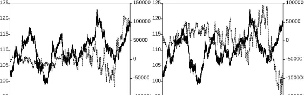
Figure 1: Continuous line is the TY future (scale in the right axe). Piecewise line is NAPM (scale in the left axe).
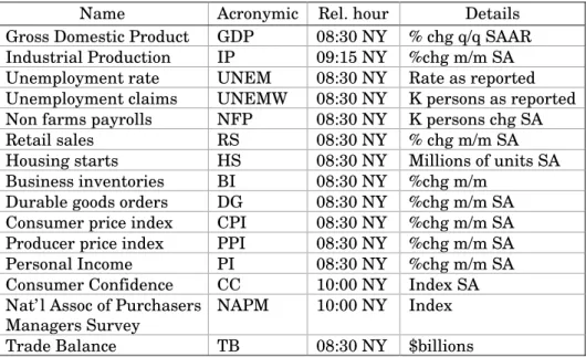
We can simplify the model (1) above in the following way. First we notice that the NAPM and the TY price are inversely correlated—see Figure one. TY moves up when NAPM goes down, peaks close to when NAPM bottoms then sells off when NAPM starts recovering again, until it reaches a top. So the business cycle factor and the price action are broadly co-integrated. Also CoT shows, especially in the last 3 years, that the amplitude of swings in the hedgers and speculators net positions have increased (for example in the last rally the net speculators long positions were at 120,000 contracts at some point which is quite unprecedented since the birth of that contract)—see Figure two. So the price trend, the macro trend and the positioning trend are strongly related and, in a way, represent the same explanatory variable. We therefore decide to subdivide the business cycle in different phases, explained below, and estimate the following equation:
[ ]
(
)
, , ( ) 0(1
)
,
p t i C S N t i t i t iL TY
β
N
−E N
−ε
=−
=
∑
−
+
(2)where i is the time measured since the moment of the release to
about 1h30 after,1 C is the variable representing where we are in the
1 The exact moment of time up to which the effect will last depends on the fundamental
business cycle and taking values “Top, Bottom, Expansion, Contraction” and S(N) is the sign of the forecast error N-E(N). Therefore (2) is a time varying parameter model, being a function of the moment in the business cycle, the sign of the forecasting error and the number of elapse periods between the macro release and the return.
The fact that parameters depend on the moment of the business cycle and the sign of the forecasting errors will permit us to discover hidden relations that otherwise are not possible to figure out. For example in the case of non farms payrolls (one of the most
important fundamental) if we do the analysis for a β independent of
C and S(N) we will find a very strong relation, as expected. However
if we permit to β depends on the business cycle and the sign of the
forecasting error, we will find that non farms payrolls matters when the cycle is in the top and the bottom, it does not matter a lot when the cycle is in expansion and it matters in the contraction when the sign of the surprise is the same to the sign of the trend. These
results are not obvious when βi,C,S(N)=βi.
95 100 105 110 115 120 125 -100000 -50000 0 50000 100000 150000 10000 20000 30000 40000 50000 60000 95 100 105 110 115 120 125 -150000 -100000 -50000 0 50000 100000 10000 20000 30000 40000 50000 60000
Figure 2: In left panel the TY future (left axe) and net CoT of speculators (right axe). In right panel TY future (left axe) and net CoT of hedgers (left axe). In both solid line is the TY future and dashed line is the net CoT.
3 Methodology
Given the previous arguments, our interest is to model the effect of the news arrival in the bond future market and analyze how it affects it not only contemporaneously but also through time, depending on the momentum of the business cycle and the sign of the forecast error. For example, for how long do employment news affect to the bond future market? Or how does the impulse effect of a CPI release look like throughout the day in the bond future market? Therefore, roughly, we want to see the effect through time of a shock of a given quantity in the bond future market.
Under the econometric point of view several alternatives arise. For example we could consider that the news arrivals and the bond future price are pure stationary time series and hence, in an univariate context, built a transfer function model, where the transfer function is the ratio of two finite polynomials yielding to an infinite polynomial and hence an infinite response.
In a more simplistic context we could consider a standard regression model with the news arrival and all its lags as exogenous variables and returns of TY as endogenous variable, yielding a model similar to (2)
[ ]
(
)
0(1
)
.
p t i t i t i t iL TY
β
N
−E N
−ε
=−
=
∑
−
+
(3)Here we assume that just one news, i.e. one macro number, arrives to the market. Notice that p should not be fixed and it should vary through macro number, i.e. the shock effect does not last for the same length for all macro numbers. The differences in p through numbers will be tested empirically.
This model, although very simple, is not adequate for several reasons. The main one is because we would like to have a smooth effect of the news shock through time and hence we would like to have some smoothness constraints between parameters instead let them to vary freely. The second reason is because the number of parameters can become large if our sample frequency is high and the effect of the fundamental on the TY stands for long.
In order to avoid these problems we use a Polynomial Distributed Lag (PDL) model, also known as Almon’s model (1965).
See, among others, Green (1993) chapter 17 and Johnston and Dinardo (1997) chapter 8.
PDL models were introduced for a different reason than the two aforementioned: many times when contemporaneous and past values of exogenous variables are introduced there can easily arise multi-collinearity problems. This does not happen in our case since the exogenous variables take value zero everywhere except when the news is released. The Almon’s model is based on the assumption that the coefficients are represented by a polynomial of small degree
2
0 1 2
,
0,
,
,
K
i
i
i
i
Ki
p
K
β α
=
+
α
+
α
+ +
!
α
=
!
>
(4)which can be expressed in matrix terms as
,
H
β
=
α
(5) where 21
0
0
0
1
1
1
1
1
2
4
2
.
1
3
9
3
1
K K KH
p
p
p
=
"
"
"
"
#
#
#
#
(6)Hence this specification permits to calculate the p coefficients estimating only K coefficients. K is an integer number usually between three and four. Which is the correct value for K? There is not a commonly accepted criteria about this point. Some authors suggest the use of F-statistics. Note that the degree of the polynomial will determine the flexibility of it. For degree zero all the
β’s will be equal and hence they form a zero slope straight line. For
degree equal one the β’s decrease or decrease uniformly. For K=2 the
β’s form a concave or convex bell. For K=3 the β’s can form a convex
shape during some periods and concave for others yielding a sort of wave whose amplitude decreases with i=1,…,p. Since a priori we believe that the effect of the news release will affect the bond future
price smoothly and with periods of positive effect and periods of negative effect, we set three as degree of the polynomial.
Next, substituting (4) in (3) we obtain
[ ]
(
[ ]
)
[ ]
(
)
0 1 0 0 3 3 0 0 ,0 1 ,1 3 ,3(1
)
,
p p t t i t i t i t i i i p t i t i t i t t t t t tL TY
N
E N
i N
E N
i
N
E N
z
z
z
AZ
α
α
α
ε
α
α
α
ε
ε
− − − − = = − − =
−
=
−
+
−
+ +
−
+
=
+
+ +
+ =
+
∑
∑
∑
!
!
(7)and the α’s can be estimated by standard OLS if the error term fulfill
the classical assumptions. Eventually if there is some autocorrelation and outliers we can enhance the model with past lags of the exogenous variable and an additional set of dummies. Some remarks can be done regarding stationarity and variance effects. With respect to stationarity the bond future prices
have an unit root. Hence (1-L)TYt=∆TYt will be stationary. The
exogenous variables are stationary since we are not analyzing the effect of the macro number on the future prices but the news, that is, the forecasting error, and it is always stationary.
Regarding the variance effects, there is clearly heteroskedasticity in the first differences of the bond future. This article is not dealing with the news effects on the volatility and hence in order to compute the optimal t-statistics for the parameters in the mean equation we use the White’s (1980) heteroskedastic consistent covariance matrix estimator which provides correct estimates of the coefficient covariances in the presence of
heteroskedasticity of unknown form:2
(
)
1 2 2(
)
1 1ˆ
'
T'
.
t t tT
Z Z
z
Z Z
T
K
αε
− − =
Σ =
−
∑
(8)2 Some other authors have used a two-step weighted least square procedure such that
they handle volatility in one of the steps. However, as Andersen et al. (2001) notice, there is no change on the qualitative results when modeling explicitly the variance or using White’s estimator.
From the estimated α’s is possible recover the estimates for
the β’s using equation (4) and their standard errors are easily
computed from those of the α’s via
ˆ
H
ˆ
H
.
β α
Σ = Σ
(9)Finally conditioning the α’s to the momentum of the business
cycle and the sign of the forecast error is direct and hence we obtain an estimation of (2), the equation of interest.
4 Data
Data are the TY and the macro numbers. They are sampled in 10 minutes from 08:20 to 12:30 NY time and from April 1992 to April 2001. Thus the sample size is 61048 observations.
They all have been extracted from the XMIM database server. It is a UNIX server with daily updated databases. The catalog contains, among others, economic indicators, equities, futures, indices and monetary indicators. From this database we extract the TY. It is traded at the Chicago Broad of Trade (CBOT) from 08:20 am to 03:00 pm, NY time.
With respect to the macro numbers, we use a priori 15 variables, which are summarized in Table one. They are extracted from the XMIM database that in his turn are extracted from MMS International, a firm that conducts a weekly survey of forecast and market sentiment from a network of 100 or so top dealers, traders and economists. The data consists of an estimate of the number, which is a median of the survey results, and the actual number expressed in the same terms as the estimate.
For our analysis we do not use the estimated neither the actual numbers but its difference that is a measure of the forecasting
error, that we refer as the news.3 The choice of the fundamentals is
done such that they represent the real economy variables (UNEM, Weekly Claims, NFP, RS, HS and BI), inflation variables (PPI, CPI),
3 Some authors, Balduzzi et al. (1999) and Anderson (2001) among others, standardize
the news dividing by its sample standard deviation. It is done only for facilitating interpretation. However we prefer not to standardize since the traders observe the net effect of a news rather than its standardize version.
supply and demand confidence variables (NAPM and CC) and
export-import variables (TB).4
Further details are needed with respect to data transformations.
For the futures contracts, some transformation is needed since they mature every three months and hence they have often different pricing. When the contract months change or expire there is a continuity problem in how to deal with these pricing gaps. We rollover the future contracts when the open interest rate becomes greater in next contract (because this usually means the following contract is the more liquid contract) using linear interpolation. For news releases, remark that data are in ten minutes interval and macro numbers are, at least, weekly released. The way we transform the macro data is the following: we reshape the macro time series to have the same number of rows as the 10 minutes bond future. Then we multiply the reshaped vector by a dummy variable that takes value one when the news is released, i.e. at the date, hour and minute is released, and zero otherwise. Then we compute the forecast error, or the news, as the difference between the actual number and the estimated one. The resulting time series is a stationary process with values equal to the forecasting error when the announcement is released. This way of building up the process and using the PDL model will permit us to measure how the news, the forecasting error, affects the bond future market contemporaneously and throughout time.
Notice that data are sampled from 08:20 am to 12:30 pm NY time, whilst the market closes at 03:00 pm. We therefore discard all the observations from 12:30 pm to 03:00 pm. It means that our data are not proper time series. The are three reasons: i)the aim of the paper is to analyze the news impact of macro numbers on the bond future prices. Indeed it turns out that the news impact only stands for a few hours and hence since most of the news are released at 08:30 AM NY time, the impact should be hardly distinguished after 12:30. ii)at this time starts lunchtime and hence the trading activity slows down sharply which implies that necessarily the news effect
4 We did not include monetary fundamentals like M1 and the Fed interest rates. The
reasons are: The former does not affect the TY and the later is not a proper fundamental but rather a reaction of the fundamentals, i.e. the Fed acts according to the fundamental releases. Therefore study the effect of the Fed targets on the TY is out of the scope of this paper.
vanishes. Finally, after lunch and before 14:00 (close) the price action may be somewhat distorted by the activity of the bond pit
locals that mostly take intra-day positions and close them towards
the end of the session and hence their activity is not related to the fundamentals releases.
In the above quoted papers on volatility and fundamentals there is always an intra-day seasonality to take into account, i.e. the variance is greater at the opening and closing than during the rest of the day. However in returns there is no seasonality. If there were seasonality it would mean that there are systematic opportunities of
profits and it goes against the marker efficiency. Therefore ∆TYt has
no seasonality.5
Some explanation on the business cycle: Where do an expansion and a contraction begin?. One possibility to decide the momentum of the economy would be to consider the NBER dates of recessions and expansions, however, as noticed by McQueen and Roley (1993), the NBER turning points only classify the direction of the cycle rather than the level. We are considering the NAPM. It is more widely used among fixed income traders than the NBER indicator since it represents more accurately the cycles of the bonds and it has been proven to provide a forward-looking indication of the business cycle direction.
We consider three different divisions of the business cycle: 1. Divide the NAPM in upward and downward trends. 2. Divide it in top, bottom and trend parts.
3. Divide it in top, bottom, expansions and contractions.
With respect to the first division we consider that a change of trend is produced when the trend change is for at least three periods, as commonly accepted among bank’s analysts.
With respect to the second and the third division some further explanation is required. As previously quoted, McQueen and Roley (1993) analyzed the effect of the news on the S&P 500 in different stages of the business cycle. They used as measure of the business cycle the IP. They determined the levels of high, medium and low economic activity estimating a trend and then fixing some intervals around the trend. This is a purely statistical method subject to the choice of the bandwidth. We believe that the right determination of
5 It has been verified, although not shown here, doing Dickey-Fuller tests for intradaily
the business cycle phases would be the one commonly accepted by the fixed income traders since they are those that generate the TY process.
Indeed the NAPM is largely used among traders as a measure of the business cycle. It is constructed from a survey which is a test with just three possible answers: better, worst or equal with respect to the previous period. With these answers a percentage is built. Therefore a percentage of 50 means that half of the respondents think that the business conditions are good whilst the other half believe the contrary. Hence a value below 50 is a signal for the traders of a weak economy. On the other hand, historical data shows that a NAPM above 54.5 is an indicator of expansion. Therefore we consider the following classification: Top if NAPM is above 55, bottom if it is below 50, expansion if it is rising and between 50 and 55, and contraction if it is falling and between 50 and 55.
Table one: Information on Macro Numbers
Name Acronymic Rel. hour Details
Gross Domestic Product GDP 08:30 NY % chg q/q SAAR
Industrial Production IP 09:15 NY %chg m/m SA
Unemployment rate UNEM 08:30 NY Rate as reported
Unemployment claims UNEMW 08:30 NY K persons as reported
Non farms payrolls NFP 08:30 NY K persons chg SA
Retail sales RS 08:30 NY % chg m/m SA
Housing starts HS 08:30 NY Millions of units SA
Business inventories BI 08:30 NY %chg m/m
Durable goods orders DG 08:30 NY %chg m/m SA
Consumer price index CPI 08:30 NY %chg m/m SA
Producer price index PPI 08:30 NY %chg m/m SA
Personal Income PI 08:30 NY %chg m/m SA
Consumer Confidence CC 10:00 NY Index SA
Nat’l Assoc of Purchasers
Managers Survey NAPM 10:00 NY Index
Trade Balance TB 08:30 NY $billions
NY stand for NY time, Rel for released, % chg percent change, SA seasonally adjusted, SAAR seasonally adjusted annual rate, m/m month to month and q/q quarter to quarter
Finally, some autocorrelation is found on the TY and one lag suffices to take it into account. This effect is usually found in stock prices. It does not mean necessarily predictive capabilities but it is due to microstructure effects (see Andersen and Bollerslev, 1998, footnote 10). Moreover our data are not time series in the proper
sense. The coefficient is statistically the same through all possible divisions and through all the numbers, meaning the independence of the exogenous variables. The coefficient of the AR(1) parameter is (in mean) –0.03457 with standard deviation of 0.006831.
5 Results
In this section we explain how to interpret the results in the Appendix’s Tables by discussing briefly the effects of each number on the TY. As mentioned earlier we divide the analysis both in function of the sign of the forecast error N-E(N) and in function of the division of the economic cycle. Four possible divisions are possible, that, for the ease of exposition, we recall here:
(1) Naive category which corresponds to no division at all (all cases).
(2) Downward and Upward trends where we subdivide according to the first period of three consecutive falling and rising NAPM.
(3) Top, Bottom and Trend where we subdivide between extreme readings of the NAPM (above 55 and bellow 50 respectively) and intermediate (between 50 and 55) ones without specifying the direction of the cycle.
(4) Top, Bottom, Downward and Upward Trends which is the most exhaustive division into the four cycle categories. The thresholds are the same as in previous division.
The way to read the tables at the end of the paper is as follows: first decide which period in the economic cycle we are interested in. For example let us look at CC (Table 2), and the
trending period of a business cycle between extremes (category 3
above which corresponds to the sub-table Top, Bottom and Trend in the upper right side). Let us now ask what is the expected response of the market to a news shock from the moment of the release to 40 minutes after. We go to the Plain , Trend column and sum the first 4
coefficients: -0.0046 - 0.0048 - 0.0043 - 0.0033=0.017. The equation is
( )
(
)
40 0
0.017
0 0 40TY
−
TY
= −
N
−
E N
+
ε
. So for example if E(N0)=105,N0=109 and TY0=100 then
E TY
(
40)
=
100 0.017 4
−
⋅ =
99.94
. Hence 99.94 is the forecasted value, ceteris paribus, of the bond fortyIf we want to be more precise and look at instances where the forecast error was positive (here it is +4), we go to the Pos, Trend column and sum the first four coefficients there:
-0.0045 - 0.0054 - 0.0051- 0.0041=0.0191 and then
E TY
(
40)
=
99.92
,which will be our more precise estimate.
We discuss now the effects of each news surprises in detail. Given the number of fundamentals we only illustrate graphically the first case, CC. Similar figures could be done for the rest. In general some comments can be drawn:
1. The signs are all, except some pathological cases, intuitively correct.
2. In almost all cases where the effect is significantly different from zero there are asymmetries.
3. In general the behaviour in the most exhaustive division is similar to the behaviour in the other divisions.
5.1 Consumer Confidence (Table 2).
Applying the above example to the whole table of Consumer Confidence we can draw the following set of conclusions. i)The sign of the coefficients is intuitively correct: Confidence higher than expected yields bond market sell-offs.
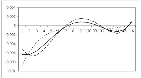
-0.01 -0.008 -0.006 -0.004 -0.002 0 0.002 0.004 1 2 3 4 5 6 7 8 9 10 11 12 13 14 15 16
Figure 3: Impulse respond function of a shock in CC on TY in division 1. Solid line considering all forecasting errors Dotted line when only considering negative forecasting errors. Dashed line when considering positive forecasting errors. Vertical axe is the coefficient, horizontal are the minutes (divided by ten) after the release.
ii)On average, and specially the first hour, the effect of a positive forecast error is larger than the effect of a negative forecast error. See Figure three. This means that for a given absolute value of forecast error (e.g. 4 points above) the bond sell-off (in case FE = +4)
is more violent than a bond rally (in case FE = -4). iii)The above holds
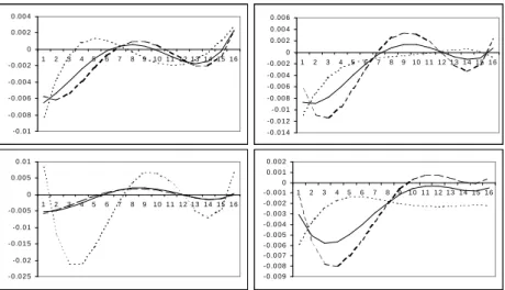
for all the economic environments save in an economic expansion. There it seems that negative forecast errors (i.e. a weaker Confidence than expected) generate bigger bond moves that a positive error. See Figure four. This is an illustration that when CC comes “against the trend” it tends to get more publicity in the bond market. Also when the economy is contracting positive forecast errors tend to impact the market more than negative (along-the-trend ones).
Figure 4: Impulse responses of TY to a shock in CC. Top left when the economy cycle is in the top. Top right when the cycle is in the bottom. Bottom left when it is in expansion and Bottom right when it is in contraction. Solid, dotted and dashed lines are the same as in Figure three. Vertical axe is the coefficient, horizontal are the minutes (divided by ten) after the release.
5.2 NAPM (Table 3)
The sign of the coefficients is intuitively correct: NAPM higher than expected yields bond market sell-offs. On average the effect of a negative forecast error is larger than the effect of a positive forecast error which means that the market rallies stronger
- 0 .0 1 - 0 .0 0 8 - 0 .0 0 6 - 0 .0 0 4 - 0 .0 0 2 0 0 .0 0 2 0 .0 0 4 1 2 3 4 5 6 7 8 9 1 0 1 1 1 2 1 3 1 4 1 5 1 6 - 0 .0 1 4 - 0 .0 1 2 - 0 .0 1 - 0 .0 0 8 - 0 .0 0 6 - 0 .0 0 4 - 0 .0 0 2 0 0 .0 0 2 0 .0 0 4 0 .0 0 6 1 2 3 4 5 6 7 8 91 0 1 1 1 2 1 3 1 4 1 5 1 6 - 0 .0 2 5 - 0 .0 2 - 0 .0 1 5 - 0 .0 1 - 0 .0 0 5 0 0 .0 0 5 0 .0 1 1 2 3 4 5 6 7 8 9 1 0 1 1 1 2 1 3 1 4 1 5 1 6 - 0 .0 0 9 - 0 .0 0 8 - 0 .0 0 7 - 0 .0 0 6 - 0 .0 0 5 - 0 .0 0 4 - 0 .0 0 3 - 0 .0 0 2 - 0 .0 0 1 0 0 .0 0 1 0 .0 0 2 1 2 3 4 5 6 7 8 9 1 0 1 1 1 2 1 3 1 4 1 5 1 6
on lower than expected NAPM than sells off on higher than expected NAPM. As in the previous fundamental the above holds for all the economic environments save the top of the economic cycle. There positive forecast errors lead a more violent response (sell-off) which is actually a bit counter-intuitive.
5.3 Non-Farm Payrolls (Table 4)
The sign of the coefficients is intuitively correct: Payrolls higher than expected yields bond market sell-offs. On average the effect of a positive forecast error is larger than the effect of a negative forecast error. The market rallies stronger on lower than expected Payrolls than it sells off on higher than expected NFP. Again the above holds for all the economic environments save in an economic contraction. There negative forecast errors (smaller NFP) induce a more violent rally in bonds. In some sense (and unlike the CC case) the NFP’s have a tendency to “accelerate” the bond trend.
5.4 Unemployment Rate (Table 5)
Again the sign of the coefficients is intuitively correct: UNEM higher than expected yields bond market rallies. The counter-intuitive signs in the “Pos, Bott” column in the last table are due to outliers and these coefficients have no statistical significance. On average the effect of a positive forecast error is larger than the effect of a negative forecast error which means that the market rallies stronger on higher than expected unemployment than sells off on lower than expected UNEM.
However the behaviour is not as good as for NFP. As they are both released at the same time we would expect similar effect on TY. It is not the case. The reasons are: i)UNEM is not seasonally adjusted by the US Census Bureau whilst the Bureau of Labour Statistics adjusts NFP. We could adjust UNEM by seasonality but it is not a good idea since it will not be what the markets observes when it is released. ii)The NFP survey has a bigger sample size (390,000 establishments) than UNEM (60,000 households) and iii)in 1994 the questionnaire and the collection method for UNEM changed introducing some disturbances on the sample. Therefore given that both measures explain the employment activity, we believe that it is more convenient to focus on NFP.
5.5 PPI, CPI (Tables 6 and 7)
Since these two fundamentals are inflation measures and results are not very far we analyze them jointly. However we concentrate only on CPI given that the PPI coefficients are not statistically significant. Probably PPI is not significant because NAPM, which is released before, is informative enough about the manufacturing sector and CPI is released just after which implies that traders still keep in mind the NAPM results as a benchmark of the manufacturing and industrial sector and they wait for the CPI to have a precise idea of the inflation.
The sign of the CPI coefficients is intuitively correct: Inflation higher than expected yields bond market sell-offs. On average the effect of a positive CPI forecast error is larger than the effect of a negative forecast error. The market sells off stronger on higher than expected inflation than it rallies on weaker than expected inflation. The above holds for all the economic environments save at the top of the economic cycle. There negative forecast errors (smaller inflation) induce a more violent rally in bonds. Maybe traders take it as a confirmation that the downward leg of the cycle has started.
5.6 Retail Sales (Table 8)
Sales higher than expected yields bond market sell-offs, due to the correct signs. On average the effect of a negative forecast error is larger than the effect of a positive forecast error. The market rallies stronger on lower than expected RS than it sells off on higher than expected RS. Finally the above holds for all the economic environments save in an economic contraction. There positive forecast errors (higher sales) induce a more violent sell off in bonds.
5.7 Industrial Production (Table 9)
The sign of the coefficients is intuitively correct: IP higher than expected yields bond market sell-offs. The only pathological case where it does not hold is for “Neg, Down” columns. On average the effect of a positive forecast error is larger than the effect of a negative forecast error. The market sells off stronger on higher than expected IP than it rallies on lower than expected IP.
The above holds for all the economic environments save on top of the economic cycle. There negative forecast errors (lower IP) induce a more violent rally in bonds. It could mean that IP is one of
the very watched signs by the market as far as cycle turns are concerned (given that it comes monthly and not quarterly like GDP).
5.8 Housing Starts, Durable Goods, Personal Income (Tables 10,11 and 12)
For all these three fundamentals the sign of the response is intuitive (positive forecast error results in bonds selling off). For HS and DG the statistical significance of the coefficients is below our acceptance threshold in the two most exhaustive divisions whilst PI has a residual importance in any divisions. In the cases of HS and DG the effect of its release has an effect for no longer than half an hour with some rebound in some cases after one hour and a half.
5.9 Weekly Unemployment Claims (Table 13)
This is the only weekly released fundamental and hence it deserves some further explanation. It is not based on a survey but on a complete register which is announced every week and hence it is a short term ongoing view of the labour market and can provide the first signals of some future change in the economy, i.e. it is a sort of leading indicator of the state of the economy, apart of the seasonality, holiday periods and some other phenomena like extreme weather conditions. Hence although it can be very useful for discover ongoing hidden problems, it is very erratic and some smoothing method can be used to obtain the latent trends. Nevertheless, as shown in Table one, this number reported by the Department of Labour is the raw change in the number of persons.
The sign of the coefficients is intuitively correct: Claims higher than expected yields bond market rallies. On average the effect of a positive forecast error is larger than the effect of a negative forecast error. The market rallies stronger on higher than expected UNEMW than it sells off on lower than expected UNEMW. The above holds for all the economic environments.
5.10 GDP, Trade Balance, Business Inventories (Table 14)
For all these three fundamentals the statistical significance of the coefficients is below our acceptance threshold and we will not push the analysis further. Indeed even in the less exhaustive case these fundamentals do not have any effect on TY (and this is why for these numbers the results for each division are missing). Some
explanation of this lack of significance is given in next subsection 5.12.
5.11 Summary
So from the analysis above we observe that some economic releases induce asymmetric responses at different parts of the economic cycle, in function of the sign of the error.
It seems like CC, RS and NFP play slightly different roles as far as the psychology of the markets is concerned: when traders react to CC and RS they seem to be looking for signs that the macro trend is turning. When they react to NFP they seem to be looking for signs that the macro trend is getting confirmed. Also it seems like IP and CPI are watched carefully close to the top of the economic cycle to see whether the cycle is about to turn.
The market also seems to have a general bias when it approaches certain numbers. We call a “Bearish Bias” a situation where the expected sell-off is bigger in magnitude than the expected rally for the same absolute value of the forecast error and the opposite sign. Also the “Bullish Bias” is where the expected rally is bigger in magnitude than the expected sell-off for the same absolute value of the forecast error and the opposite sign. Across all the sample we draw the conclusions that there is a
(1) “Bearish Bias” for news coming from: CC, CPI, and IP.
(2) “Bullish Bias” for news coming from: UNEM, NAPM, NFP, RS and UNEMW.
5.12 Timeliness
From the above conclusions it seems that results are mixed. Some fundamentals have a definitive effect on TY whilst there is no effect at all for some others. Even some results seem counter intuitive. Could we expect that GDP, the classical measure of the economy, is totally innocuous to TY, one of the most heavily traded long-term interest rate contracts in the world?, or that the TB, the most important indicator of the import-exports, is irrelevant for the behaviour of TY?, or that CC, a fundamental based on a naïve survey based in turn on opinions, has more effect that PI?.
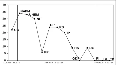
The answer is on Figure five. It is the total number of significant parameters for each fundamental given division 4 and ordered temporally according to when they are released. In general the importance of the fundamental decreases as the time interval
between its release and the period it is covering increases. This effect is called timeliness and it has been found previously by other authors, see for example Flemming and Remolona (1997).
Timeliness, in this context, just means that traders are not interested by information about the state of the economy at some point in time and if it is released some months after. On the contrary the sooner the fundamental is released the more it is perceived important by traders and hence the more effect it has on TY. It is the case of CC which is released in the month it is covering. Although CC is not a “big one”, it conveys a lot of fresh information about the state of the economy that is rapidly absorbed by traders and used to trade. The contrary example is the GDP. It is released around one month and a half after the period it is covering. Given that it is the tenth fundamental (among the chosen for the analysis) to be released it does not really add information and hence agents do not react when it is released. Moreover GDP is quarterly released and continuously revised, being another reason for the lack of interest in this fundamental.
Figure 5: Timeliness. Each point represents the number of significative coefficients in division four, the most exhaustive. The vertical lines represent the month that they released. Within the lines they are temporally ordered as they use to appear. For example, CC is released at the end of the month it is covering and BI and TB two months later. Notice that i)PI is in the frontier between one and two months because it is sometimes released within one month and other within two months and ii)UNEMW is nor present since it is released weekly.
CC UNEM NF PPI IP HS DG TB BI PI GDP CPI NAPM RS 0 5 10 15 20 25 30 35 40
CURRENT MONTH ONE MONTH LATER TWO MONTH LATER
CC UNEM NF PPI IP HS DG TB BI PI GDP CPI NAPM RS 0 5 10 15 20 25 30 35 40
6 Reality Check
All above results are under a quite constrained model. First the model is linear in the variables and second it imposes some smoothness conditions on the parameters.
A natural question would be how good the model predicts and it the decaying pattern of the parameters represents the true behaviour of TY. In other words, is the model a good short-run predictor of TY after a macro release?. Due to the smoothness constraints the model will predict smoothly . The corner stone here is not the exact prediction of the return but a short-run prediction of TY in levels that will tell us which is the net effect of the shock given by the fundamental release.
Another natural questions that arises is the following: is it really worthwhile the differentiation of TY depending on the business cycle?, is there some value added disentangling TY depending on the economic cycle’s phases?.
In order to answer to these questions we do a prediction exercise based on real data and the estimated parameters. As in previous section we will focus in one fundamental but similar exercise can be done for the others. Previously we have focused on CC. Now we will analyze the effect of NFP. We chose this fundamental because as shown above it is one of the most important and, on the other hand, using another different to CC we diversify the in deep analysis.
We chose as date of release August first 1997. At this date the business cycle was on the top (the NAPM was 58.6) the NFP released was 316,000 whilst the expected number was 197,500. Hence the
forecasting error was 118,500 and therefore positive.6
Model (2) is transformed in levels for prediction of TYt rather
than ∆TYt and introducing the autoregressive component mentioned
earlier:
(
)
1 2 , , ( ) 0(1
)
.
p t j t j t j i C S N t j i t j i t j iE TY
+α
E TY
+ −α
E TY
+ −β
N
+ −E N
+ −ε
+ =
= +
−
+
−
+
∑
Notice that the prediction is not one-step but jth-step, that is when forecasting TY at time j we use the predictions at time j-1 and
j-2 rather than the observed data. Notice that, given the model, the
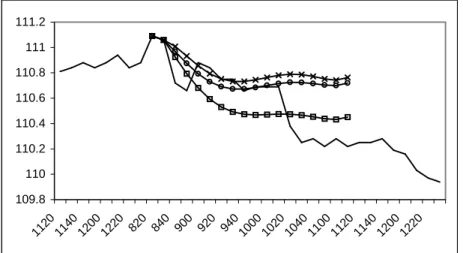
one-step forecast would be fully dominated by the observed data and hence there will not be almost effect of the releases on the TY. Figure six represents the forecasting exercise under different scenarios, from the most favourable to the less favourable with the naïve case in the middle. The most favourable case corresponds to the sub division according with the real data, i.e. to the estimation when the economy cycle is in the top phase and the forecasting error is positive. It is the line with squares. For comparison purposes we include other two cases: the most naïve case (line with circles) and the antagonist, that is using the estimated parameters when the forecasting error is negative and the economic cycle is in the bottom (line with crosses). Finally in Figure six there is also, for illustration purposes, the path of TY during the previous day and the day after the release. 109.8 110 110.2 110.4 110.6 110.8 111 111.2 1120 1140 1200 1220 820 840 900 920 940 1000 1020 1040 1100 1120 1140 1200 1220 Figure 6: Solid line represents the observed TY. Squared, circled and crossed lines are the predicted TY under the following scenarios: respectively i)positive forecasting errors and top part of the cycle, ii)plain and iii)negative forecasting errors and bottom part of the cycle.
By far the estimated parameters taking into account the sign of the forecasting error and the momentum of the cycle is the best predictor and it follows, although smoothly, the path of the TY after the release. For example during the first half hour the slope of this estimate is more pronounced than the slope of the other two
predictors. Moreover after two hours the net effect is more accurate than in the other cases.
Hence disentangling between the sign of the forecasting error and the phase of the economic cycle is important for prediction purposes.
7 Conclusions
When dealing with the analysis of intra-day bond prices, it seems reasonable to believe that on this short time scale movements are produced by small shocks whose effects stand in the market for some hours. These shocks can be, among others, political events, natural catastrophes, rumors, macro releases, etc. Among all, the macro releases are the only ones that arrive to the market systematically every week, month or quarter. Moreover as their time of arrival is known with certitude, agents can form systematic expectations about them.
Therefore if a macro release is far from the expected number, agents will react as something unexpected happened. These reactions, on the TY bond future, have been measured here. Results show that the traders react when the forecasting error is different from zero. Moreover it is shown that the reaction of the TY to a forecasting error is different depending on whether it is positive or negative and, most importantly, the reaction varies significantly depending on the momentum of the economic cycle measured via the Nat’l Assoc of Purchasers Managers Survey (NAPM).
It is also found that the time of the release matters and the closer it is to the covering period, the more effect it has on the TY. Finally a prediction exercise shows that the sign of the forecasting error and disentangling the momentum of the economic cycle is important for predicting accurately the price reaction to the macro release.
Some future research is possible. From the financial point of view some more formal theoretical framework could be set up and one could try to infer the parameters of the structural model (1) from the estimated ones in (3). Under the econometric point of view it would be possible to do some bootstrap estimation since the disaggregated level of the cycle is exhaustive and in some cases there are not many data, although the sample size stands for 9 years.
Bibliography
Andersen, T.G and T. Bollerslev, 1998, Deutsche Mark-Dollar Volatility: Intraday Activity Patterns, Macroeconomic Announcements, and Longer Run Dependencies, The Journal of
Finance, vol LIII, No. 1, 219-265.
Andersen, T.G., T. Bollerslev, F.X. Diebold and C. Vega, 2001, Micro Effects and Macro Announcements: Real-Time Price Discovery in Foreign Exchange, Mimeo.
Balduzzi, P., E.J. Elton and T.C. Green, 1999, Economic News and Yield Curve: Evidence from the US Treasury Market,
Journal of Financial and Quantitative Analysis, forthcoming.
DeGennaro, R.P. and R.E. Shrieves, 1997, Public Information releases, private information arrival and volatility in the foreign exchange market, Journal of Empirical Finance 4, 295-315.
Flemming, M.J. and E.M. Remolona, 1997, What moves the Bond Market?, FRBNY Economic Policy Review, December.
Goodhart, C.A.E., S.G. Hall., S.G.B. Henry and B. Pesaran, 1993, News effects in a high frequency model of the sterling-dollar exchange rate, Journal of Applied Econometrics, vol 8, 1-13
Green, W.H, 1993, Econometric Analysis, 3rd ed. (Prentice-Hall).
Haustch, N. and D. Hess, 2001, What’s Surprising about Surprises?. The Simultaneous Price and Volatility Impact of Information Arrival, Working Paper Center of Finance and Econometrics. University of Konstanz.
Johnston, J, and J. Dinardo, 1997, Econometric Methods, 4th ed.
(Mc Graw Hill).
Li, L. and R.F. Engle, 1998, Macroeconomic Announcements and Volatility of Treasury Futures, UCSD Discussion Paper 98-27. McQueen, G. and V.V. Roley, 1993, Stock Prices, News and
Business Conditions, The Review of Financial Studies, vol 6, Number 3, 683-707.
Niemira, M.P and G.F. Zukowsky, 1998, Trading the fundamentals, (McGraw Hill).
White, H, 1980, A Heteroskedasticity-Consistent Covariance Matrix and a Direct Test for Heteroskedasticity, Econometrica, 48, 817– 838.
Table 2. Consumer Confidence
NAIVE CASE DOWNWARD AND UPWARD TRENDS TOP, BOTTOM AND TREND
Plain Pos Neg Plain, Upw Plain, Down Pos, Upw Neg, Upw Pos, Down Neg, Down Plain, Top Plain, Bott Plain, Trend Pos, Top Neg, Top Pos, Bott Neg, Bott Pos, Trend Neg, Trend 10 min -0,0063 -0,0051 -0,0087 -0,0067 -0,0060 -0,0061 -0,0093 -0,0040 -0,0085 -0,0069 -0,0085 -0,0046 -0,0057 -0,0096 -0,0064 -0,0104 -0,0045 -0,0048 20 min -0,0064 -0,0067 -0,0058 -0,0065 -0,0063 -0,0064 -0,0068 -0,0070 -0,0054 -0,0064 -0,0087 -0,0048 -0,0061 -0,0073 -0,0109 -0,0068 -0,0054 -0,0024 30 min -0,0055 -0,0065 -0,0036 -0,0054 -0,0057 -0,0055 -0,0048 -0,0076 -0,0032 -0,0053 -0,0077 -0,0043 -0,0053 -0,0053 -0,0115 -0,0043 -0,0051 -0,0008 40 min -0,0042 -0,0052 -0,0022 -0,0038 -0,0045 -0,0040 -0,0033 -0,0066 -0,0019 -0,0038 -0,0060 -0,0033 -0,0039 -0,0036 -0,0096 -0,0028 -0,0041 0,0002 50 min -0,0027 -0,0034 -0,0014 -0,0022 -0,0031 -0,0022 -0,0022 -0,0047 -0,0011 -0,0023 -0,0040 -0,0021 -0,0022 -0,0024 -0,0063 -0,0019 -0,0028 0,0007 60 min -0,0013 -0,0015 -0,0009 -0,0007 -0,0018 -0,0005 -0,0015 -0,0026 -0,0007 -0,0010 -0,0020 -0,0010 -0,0007 -0,0016 -0,0028 -0,0013 -0,0014 0,0007 70 min -0,0002 0,0001 -0,0007 0,0004 -0,0006 0,0008 -0,0011 -0,0007 -0,0006 0,0000 -0,0004 -0,0001 0,0004 -0,0011 0,0003 -0,0010 -0,0002 0,0004 80 min 0,0006 0,0012 -0,0007 0,0011 0,0002 0,0016 -0,0010 0,0007 -0,0006 0,0004 0,0008 0,0005 0,0010 -0,0010 0,0025 -0,0008 0,0006 0,0000 90 min 0,0009 0,0016 -0,0007 0,0012 0,0006 0,0018 -0,0010 0,0014 -0,0006 0,0004 0,0013 0,0007 0,0011 -0,0012 0,0034 -0,0006 0,0010 -0,0006 100 min 0,0007 0,0015 -0,0008 0,0009 0,0005 0,0014 -0,0011 0,0015 -0,0006 0,0000 0,0013 0,0006 0,0007 -0,0015 0,0031 -0,0003 0,0010 -0,0012 110 min 0,0003 0,0007 -0,0008 0,0003 0,0002 0,0007 -0,0012 0,0008 -0,0006 -0,0006 0,0009 0,0002 -0,0001 -0,0019 0,0018 0,0001 0,0006 -0,0017 120 min -0,0004 -0,0003 -0,0007 -0,0005 -0,0003 -0,0003 -0,0013 -0,0002 -0,0005 -0,0014 0,0001 -0,0004 -0,0010 -0,0022 -0,0002 0,0004 0,0000 -0,0020 130 min -0,0010 -0,0012 -0,0006 -0,0012 -0,0009 -0,0012 -0,0011 -0,0012 -0,0004 -0,0019 -0,0007 -0,0010 -0,0017 -0,0022 -0,0022 0,0006 -0,0007 -0,0021 140 min -0,0013 -0,0017 -0,0004 -0,0014 -0,0012 -0,0016 -0,0007 -0,0018 -0,0003 -0,0018 -0,0012 -0,0012 -0,0018 -0,0017 -0,0032 0,0006 -0,0011 -0,0017 150 min -0,0008 -0,0012 -0,0002 -0,0008 -0,0009 -0,0010 0,0001 -0,0013 -0,0003 -0,0006 -0,0009 -0,0010 -0,0007 -0,0006 -0,0021 0,0002 -0,0010 -0,0008 160 min 0,0008 0,0011 0,0000 0,0012 0,0003 0,0012 0,0015 0,0010 -0,0006 0,0020 0,0006 0,0002 0,0022 0,0016 0,0024 -0,0010 0,0001 0,0006
TOP, BOTTOM, DOWNWARD AND UPWARD TRENDS
Plain, Top Plain, Bott Plain, Down Plain, Upw Pos, Top Neg, Top Pos, Bott Neg, Bott Pos, Down Neg, Down Pos, Up Neg, Up 10 min -0,0066 -0,0087 -0,0030 -0,0051 -0,0057 -0,0083 -0,0063 -0,0109 -0,0014 -0,0059 -0,0056 0,0084 20 min -0,0053 -0,0089 -0,0050 -0,0049 -0,0061 -0,0036 -0,0109 -0,0070 -0,0058 -0,0038 -0,0046 -0,0126 30 min -0,0038 -0,0078 -0,0058 -0,0039 -0,0054 -0,0007 -0,0114 -0,0044 -0,0077 -0,0024 -0,0032 -0,0211 40 min -0,0024 -0,0060 -0,0057 -0,0025 -0,0039 0,0008 -0,0095 -0,0028 -0,0080 -0,0017 -0,0017 -0,0210 50 min -0,0011 -0,0040 -0,0050 -0,0009 -0,0023 0,0013 -0,0063 -0,0018 -0,0070 -0,0014 -0,0003 -0,0160 60 min -0,0002 -0,0020 -0,0040 0,0004 -0,0008 0,0011 -0,0028 -0,0012 -0,0055 -0,0013 0,0008 -0,0088
70 min 0,0004 -0,0003 -0,0029 0,0014 0,0003 0,0005 0,0003 -0,0009 -0,0037 -0,0015 0,0016 -0,0016 Plain means no difference between positive
80 min 0,0006 0,0008 -0,0019 0,0020 0,0010 -0,0003 0,0025 -0,0007 -0,0020 -0,0017 0,0019 0,0038 and negative forecasting errors
90 min 0,0003 0,0014 -0,0011 0,0020 0,0010 -0,0010 0,0035 -0,0005 -0,0006 -0,0020 0,0019 0,0067 Pos means positive forecasting errors
100 min -0,0002 0,0014 -0,0006 0,0016 0,0005 -0,0016 0,0031 -0,0003 0,0003 -0,0021 0,0014 0,0067 Neg means negative forecasting error
110 min -0,0008 0,0009 -0,0003 0,0009 -0,0003 -0,0019 0,0018 0,0000 0,0008 -0,0022 0,0007 0,0040 Top means bottom part of the cycle
120 min -0,0014 0,0000 -0,0003 -0,0001 -0,0012 -0,0018 -0,0002 0,0003 0,0008 -0,0023 -0,0001 -0,0003 Bott means bottom part of the cycle
130 min -0,0017 -0,0008 -0,0005 -0,0010 -0,0020 -0,0013 -0,0022 0,0005 0,0005 -0,0022 -0,0008 -0,0047 Down means Downward part of the cycle
140 min -0,0015 -0,0013 -0,0007 -0,0015 -0,0020 -0,0003 -0,0033 0,0005 0,0001 -0,0021 -0,0013 -0,0070 Upw means upward part of the cycle
150 min -0,0002 -0,0010 -0,0008 -0,0012 -0,0009 0,0010 -0,0022 0,0002 -0,0001 -0,0021 -0,0011 -0,0043 NET means accumulated effect for 60 minutes