O
pen
A
rchive
T
OULOUSE
A
rchive
O
uverte (
OATAO
)
OATAO is an open access repository that collects the work of Toulouse researchers and
makes it freely available over the web where possible.
This is an author-deposited version published in :
http://oatao.univ-toulouse.fr/
Eprints ID : 13910
To cite this version :
Ramiro, Victor and Dang, Dinh Khanh and
Baudic, Gwilherm and Pérennou, Tanguy and Lochin, Emmanuel
A Markov chain model for drop ratio on one-packet
buffers DTNs.
In: IEEE WoWMoM Workshop on Autonomic and Opportunistic
Communications (AOC), 14 June 2015 (Boston, United States
)
Any correspondance concerning this service should be sent to the repository
administrator:
[email protected]
A Markov chain model for drop ratio on one-packet
buffers DTNs
Victor Ramiro
⇤, Dinh-Khanh Dang
⇤, Gwilherm Baudic
⇤, Tanguy P´erennou
⇤, Emmanuel Lochin
⇤⇤Universit´e de Toulouse, ISAE-SUPAERO, France
{first.second}@isae.fr
Abstract—Most of the efforts to characterize DTN routing are focused on the trade-off between delivery ratio and delay. Buffer occupancy is usually not considered a problem and most of the related work assumes infinite buffers. In the present work, we focus on the drop ratio for message forwarding considering finite buffers. We model message drops with a continuous time Markov chain (CTMC). To the best of our knowledge, there is no previous work with such approach. We focus on the worst case with 1-packet buffers for message forwarding in homogeneous inter-contact times (ICT) and 2-class heterogeneous ICT. Our main contribution is to link the encounter rate(s) with the drop ratio. We show that the modeled drop ratio fits simulation results obtained with synthetic traces for both cases.
Keywords—DTN, Modeling, Characterization, Drop ratio, Con-tinuous time Markov chain
I. INTRODUCTION
Delay Tolerant Networks (DTNs) are a well-known paradigm to allow communication between peers when in-frastructure is scarce [1]. Communications are handled in a store-carry-and-forward format in DTNs. Hence, we benefit from peers communication opportunities (given by node move-ments, periodicity of contacts/connections, etc) to deliver data. Usually, it is not possible to establish a direct end-to-end path between source and destination; instead, a spatio-temporal path may be created by contact opportunities.
The DTNs pure definition based on the delay tolerance na-ture of communications covers a big spectrum of networks [2]: space communications, vehicular networks, sensor networks, opportunistic networks, etc. All these scenarios have in com-mon to impose strong restrictions on the resources available to the nodes (energy, memory, processing power). Many works have focused on those different restrictions providing a better understanding in terms of characterization, mobility, energy consumption, or performance metrics such as delay, delivery or drop ratios to name a few.
A pioneering work in the field of DTN performance modeling was [3], where the authors provide a Markov model for the 2-hop and unrestricted multicopy routing protocols in the case of homogeneous exponentially distributed intercontact times (ICTs). Markov modeling was subsequently applied to Epidemic routing [4]–[6], Spray And Wait [7], [8] and Binary Spray and Wait [9]. Other modeling tools include Ordinary Differential Equations [10], [11] or Petri Nets [12].
Such works showed that unrestricted buffers and epidemic routing will provide the best delivery ratio [10], even though the number of message copies increases exponentially, as predicted by the SIR (Susceptible-Infected-Recovered) model
[13]. The buffer occupancy is usually not considered a prob-lem, or one of less importance, to the point that most of the related work assumes infinite buffers [3]–[9], [14]–[17]. Heterogeneous ICTs, either for pairs [9], [15], [16] or groups [5], [14], [17] of nodes, are also rarely considered. A more detailed literature overview can be found in Table I.
We focus our work on a specific type of sensor net-work where mobile nodes perform a measurement and then transmit their data by message forwarding among their peers. Two groups of nodes are considered: sources which perform measurements, and destinations acting as collection points. A message can reach any collection point, as in an anycast network. We study the behavior of message forwarding in terms of number of dropped messages when we increase the number of messages generated in this sensor network. We use simple forwarding of messages to avoid including new message copies in the network (via replication), as this would only increase the probability of dropping a message.
We restrict our study to networks where nodes can carry only one message. Although it might seem limited, this case captures the situation of bigger buffers almost filled up with messages, to the point that every node has at most one free space in its buffer. Somehow this represents the basic limits of a DTN in terms of absorption capabilities: after reaching a given buffer occupancy, no more messages can be injected unless nodes start dropping messages due to buffer saturation. In Section II we propose a continuous time Markov chain (CTMC) to characterize the drop of messages in 1-message
buffers DTNs. The objective is to exhibit an upper bound
to the drop ratio. From this, we can extract the trade-off between the number of sources and destinations nodes in order to achieve a desired drop ratio. We show that the outputs of the CTMC model fit to DTN simulation outputs (Section III). Our contribution is twofold:
1) We study a DTN network where nodes can store only
one message in their buffer. Messages are forwarded from source to destination. Encounters between nodes are homogeneous. We model the drop ratio when increasing the number of messages (Section II-B), and provide simulations that match this dropping model (Sections III-A and III-B);
2) We extend our model to the case where nodes are
divided among two groups with different encounter rates (Section II-C). We provide simulations to com-pare with the extended model (Section III-C).
Table I: Previous literature considering finite/infinite buffers. Only [10] characterizes the drop ratio with finite buffers, using ODEs and focusing on homogeneous ICT and epidemic routing.
Reference Buffer size Exponential parameters Routing protocols Delay Delivery ratioPerformance metrics derivedNumber of copies Drop ratio
[10] Finite Homogeneous Epidemic X - X X
[11] Finite Homogeneous Spray and Wait X - -
-[12] Finite Homogeneous Epidemic, 2-hop X X -
-[18] Finite Not mentioned 2-hop X - -
-[3]–[9], [14]–[17] Infinite - - X X X
-This paper Finite Two-class HeterogeneousHomogeneous Forwarding - - - X
II. DROPMESSAGEMODEL
In this section, we define the basic notation and global hypotheses of the model. Then we introduce the specifics of our model for two cases: homogeneous intercontact time distribution and a restricted heterogeneous case with two classes of nodes.
A. Model basics
We consider a DTN with N identical nodes N = {1, 2, 3, . . . , N} with a buffer capacity of one message. We consider S < N message sources and M initial copies of the same message. Notice that S = M due to the buffer restriction. The M messages are delivered to any of D < N S destinations. Unless stated differently, we consider D = 1. Intermediary nodes act as forwarders of those M messages. Hence, no extra copies are created in the evolution of the process. The goal is to determine the distribution of dropped messages and the drop ratio over time.
Let 0 ti,j(1) ti,j(2) < ...be the successive encounter
times among nodes i and j. We consider that the transmission time of a message is negligible with respect to the time it takes to two nodes to meet one another. It follows that the n-th
inter-contact time between i and j is icti,j(n) = ti,j(n+1) ti,j(n).
Later we set specific hypotheses on the nature of the processes
{ti,j}. Since each node can keep only one message, each time
a contact occurs we try to forward it. Hence, when node i and
j meet either: (i) only one of the nodes has a message, it is
instantaneously transmitted, or (ii) both nodes have a message, then one is chosen at random to instantaneously transmit its message while the other drops its message.
B. The (d, c) model: homogeneous case
For the homogeneous case, we assume that the processes
{ti,j(k), k 1, 8i 6= j 2 N } are mutually independent
and homogeneous Poisson processes with rate > 0. Hence
the random variables {icti,j(k), k 1, 8i 6= j 2 N } are
mutually independent and exponentially distributed with mean
1/ .
To calculate the number of dropped messages, we introduce a continuous time Markov chain (X(t), t > 0). The states of the chain are (d, c), where d represents the number of dropped messages and c the number of message copies. Our initial state is (0, M). The transitions from a state (d, c) are either to (d, c 1) when a message is delivered or to (d + 1, c 1) when a drop occurs. The rate to encounter a destination will be D . Since we have c nodes with a copy of the message, the former transition will happen with rate cD . The latter occurs
with rate c(c 1)
2 given the number of combinations where
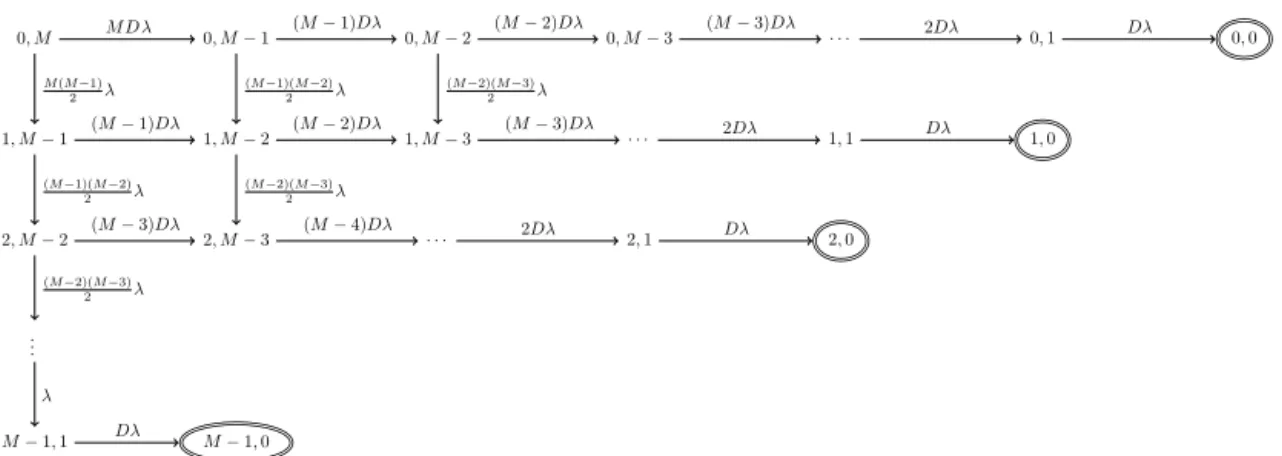
two nodes with a message meet. In Figure 1, we detail the possible transitions for the general case. The absorbing states of the chain are in the form (d, 0) with 0 d M 1. Notice that when reaching the absorbing states, we must impose some border conditions. Since the last message will be delivered with probability 1, we cannot transit from state (d, 1) to (d + 1, 0). In Figure 2, we draw the complete Markov chain for M.
d, c d, c 1 d + 1, c 1 d + 1, c 2 cD c(c 1) 2 . . . . . . . . . . . . . . . · · ·
Figure 1: Chain transitions from a given state (d, c). Either a destination is found among D possibilities, leading to state
(d, c 1), or there is a drop, leading to (d + 1, c 1). State
(d + 1, c 2) is included to show the progression of states.
We can easily calculate the probabilities of going out from the state (d, c). Indeed, the embedded Markov chain for X(t) allows to write the probabilities to jump between states as shown in (1). P ((d, c)! (d, c 1)) = cD cD +c(c 1)2 = 2D c + 2D 1 P ((d, c)! (d + 1, c 1)) = c(c 1) 2 cD +c(c 1)2 = c 1 c + 2D 1 (1a) The absorbing states probabilities are defined as:
PM(d) = P (X1= (d, 0)|X(0) = (0, M)), 0 d M 1
(2) Since the process is a feed-forward process, these proba-bilities can be easily calculated with a dynamic programming algorithm. The drop rate distribution is defined as the expected value of reaching the absorbing states over the number of
starting messages 1
M
PM 1
0, M 0, M 1 0, M 2 0, M 3 · · · 0, 1 0, 0 1, M 1 1, M 2 1, M 3 · · · 1, 1 1, 0 2, M 2 2, M 3 · · · 2, 1 2, 0 ... M 1, 1 M 1, 0 M D (M 1)D (M 2)D (M 3)D 2D D (M 1)D (M 2)D (M 3)D 2D D (M 3)D (M 4)D 2D D M (M 1) 2 (M 1)(M 2) 2 (M 2)(M 3) 2 (M 1)(M 2) 2 (M 2)(M 3) 2 (M 2)(M 3) 2 D
Figure 2: Complete Markov chain for the drop process. When there are no more messages to deliver, we reach a final state (d, 0) with d being the number of messages dropped.
It is important to notice that the probabilities are
indepen-dent of the process arrival rate . Therefore, for any {ti,j}
defined as before, we expect the same drop ratio results.
C. The (d, c1, c2)model: heterogeneity with two classes
We extend the (d, c) model to the case of two different
classes of nodes C1 and C2, with |C1| = N1 and |C2| = N2
such that N = N1+ N2+ D. For convenience, we impose
D = 1. To keep the problem symmetrical, the destination does
not belong to any class of nodes. We have M = M1+ M2
messages distributed as M1 in C1 and M2 in C2.
The heterogeneity is defined such that the processes {ti,j}
have different rates for each class: independent homogeneous
Poisson processes with rate 1 in class C1 and with rate
2 in class C2, while inter-class interactions are given by
independent and homogeneous Poisson processes with rate
. As before, it follows that the random variables icti,j are
mutually independent and exponentially distributed with the
reciprocal of 1, 2 or according to the case.
The differences between the values of 1, 2and define
different speeds for the group encounter rates (and hence the waiting times between connections). For instance, this allows to model one group that will deliver its messages faster than the other. A faster delivery implies having more nodes with free buffers, hence reducing the probability of drops. The inter-class communication allows to balance the drops allowing to pass messages from one class to another. From the symmetry
of the problem, the destination meets nodes from C1 with rate
1 and nodes from C2with rate 2. This restriction can easily
be removed and does not affect the general result.
We model the states as (d, c1, c2) where d is the number
of drops, c1 is the number of copies in class C1 and c2 is the
number of copies in class C2. We identify three different kinds
of transitions from the state (d, c1, c2):
1) Delivery transitions: we meet a destination with rates
i in class Ci. Since we have ci message copies it
follows that the transitions rate are c1 1 for (d, c1
1, c2)and c2 2 for (d, c1, c2 1);
2) Drop transitions: the number of combinations in
class Ci where two nodes having a message meet
is ci(ci 1)
2 i. Also we count the c1c2 combinations
where two nodes from different classes having a
message meet with rate /21. It follows that the
transition rates are c1(c1 1) 1/2 + c1c2 /2 for
(d + 1, c1 1, c2)and c2(c2 1) 2/2 + c1c2 /2for
(d + 1, c1, c2 1);
3) Inter-class transitions: in this case we count the
number of combinations where a node from class Ci
passes a message to a free node from class Cj6=i. This
happens ci(Nj cj)times with rate . It follows that
the transition rates are c1(N2 c2) for (d, c1 1, c2+
1) and c2(N1 c1) for (d, c1+ 1, c2 1).
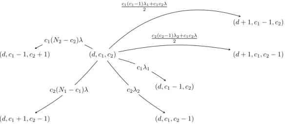
Figure 3 presents the general transitions from a state
(d, c1, c2) to all possible states described before. Same as
before, we have M absorbing states in the form (d, 0, 0) with
0 d M 1. Notice that we arrive to the absorbing state
either from (d, 1, 0) with rate 1 or from (d, 0, 1) with rate
2. Again, we need to rule out some transitions. For instance
from (d, N1, c2)we cannot go to (d, N1+ 1, c2 1) or from
(d, 0, c2) to (d, 1, c2+ 1). We do not present the complete
chain due to the impossibility to draw it because of its size. To calculate the dropping probabilities, we use the fact that the chain previously defined is an absorbing Markov chain. We
do the following: (i) enumerate the Nsvalid states of the chain
(d, c1, c2)with 0 d M 1, 0 c1 N1 and 0 c2
N2. This allows to define the mapping from 1 i Ns to
state si= (d0, c01, c02) for all the valid states in the chain. (ii)
define the matrix A with coefficients aij as the rate transform
from state si to state sj and the matrix R with coefficients rij
as the rate from state si to absorbing state s⇤j. Notice that the
size of matrix A is Ns⇥ Nsand the matrix R is M ⇥Ns. (iii)
finally, we define B = (I A) 1R where the ithrow is the
distribution of absorbing states if the initial state is si. Since
the absorbing states correspond to drop states, it follows that
B is the dropping distribution PM(d).
1We can split the inter-class Poisson processes into two counting processes
with rate p and (1 p). The splitting probability corresponds to the drop probability when two nodes have a message. Since we take one at random,
(d + 1, c1 1, c2) (d, c1 1, c2+ 1) (d, c1, c2) (d + 1, c1, c2 1) (d, c1 1, c2) (d, c1+ 1, c2 1) (d, c1, c2 1) c1 1 c2 2 c1(c1 1) 1+c1c2 2 c2(c2 1) 2+c1c2 2 c1(N2 c2) c2(N1 c1)
Figure 3: Chain transitions from a given state (d, c1, c2). We observe the increase in number of states and transitions w.r.t the
(d, c) model shown in Figures 1 and 2: inter-class transitions (d, c1 1, c2+ 1) and (d, c1+ 1, c2 1); delivery transitions
(d, c1 1, c2)and (d, c1, c2 1); and drop transitions (d + 1, c1 1, c2)and (d + 1, c1, c2 1).
III. SIMULATIONSETUP
In this section, we present the main results of the com-parison between a simulated DTN network and the modeled CTMC results. We generate pairwise ICTs distributed as defined in Section II. We then run an event driven simulation to perform the forwarding of the messages in the network and calculate the drop ratio for a given configuration. We compare the simulated and predicted drop ratio for both (d, c)
and (d, c1, c2) models. Table II presents an overview of the
simulations we cover in this section. The model results have been obtained with MATLAB, while the continuous time simulations are implemented with R.
We run all simulations with N = 100 nodes and buffer size B = 1. We repeat each simulation 10 times and provide the average results within a 95% confidence level. The network occupancy is defined as ⇢ = S/N. Sources are increased to represent the following percentages ⇢ 2 {1, 2, 5, 10, 15, . . . , 80, 95, 98}. ⇢ D Model Parameters E1 % 1 (d, c) = 500 E2 % % (d, c) = 500 E3 % 1 (d, c1, c2) 1= 2.5, 2= 200, = 66.6 E4 % 1 (d, c1, c2) 01= 10, 02= 100, 0= 55
Table II: Summary of simulations and their parameters (⇢: network occupancy, D: destinations, %: increasing).
A. Homogeneous case: single destination
As defined in Table II, we present the results of
simu-lation E1 with = 500. As said in Section II, we assume
that all pairs follow the homogeneous case with {ti,j ⇠
P oissonP rocess( )} and {icti,j⇠ exp( 1)}.
Figure 4 shows how increasing the number of sources (hence the network occupancy) increases the drop ratio, as predicted by the (d, c) model. In this figure we plot the drop ratio for each repetition (red points). We also plot the
● ● ● ● ● ● ● ● ● ● ● ● ● ● ● ● ● ● ● ● ● ● ● ● ● ● ● ● ● ● ● ● ● ● ● ● ● ● ● ● ● ● ● ● ● ● ● ● ● ● ● ● ● ● ● ● ● ● ● ● ● ● ● ● ● ● ● ● ● ● ● ● ● ● ● ● ● ● ● ● ● ● ● ● ● ● ●● ● ● ● ● ● ● ● ● ● ● ● ● ● ● ● ● ● ● ● ● ● ● ● ● ● ● ● ● ● ● ● ● ● ● ● ● ● ● ● ● ● ● ● ● ● ● ● ● ● ● ● ● ● ● ● ● ● ● ● ● ● ● ● ● ● ● ● ● ● ● ● ● ● ● ● ● ● ● ● ● ● ● ● ● ● ● ● ● ● ● ● ● ● ● ● ● ● ● ● ● ● ● ● ● ● ● ● ● ● ● ● ● ● ● ● ● ● ● ● ● ● ● ● ● ● ● ● ● ● ● ● ● 0.04 0.04 0.04 0.04 0.04 0.04 0.04 0.04 0.04 0.04 0.04 0.04 0.04 0.04 0.04 0.04 0.04 0.04 0.04 0.04 0.04 0.04 0.04 0.04 0.04 0.04 0.04 0.04 0.04 0.04 0.04 0.04 0.04 0.04 0.04 0.04 0.04 0.04 0.04 0.04 0.04 0.04 0.04 0.04 0.04 0.04 0.04 0.04 0.04 0.04 0.04 0.04 0.04 0.04 0.04 0.04 0.04 0.04 0.04 0.04 0.04 0.04 0.04 0.04 0.04 0.04 0.04 0.04 0.04 0.04 0.04 0.04 0.04 0.04 0.04 0.04 0.04 0.04 0.04 0.04 0.04 0.04 0.04 0.04 0.04 0.04 0.04 0.04 0.04 0.04 0.04 0.04 0.04 0.04 0.04 0.04 0.04 0.04 0.04 0.04 0.04 0.04 0.04 0.04 0.04 0.04 0.04 0.04 0.04 0.04 0.04 0.04 0.04 0.04 0.04 0.04 0.04 0.04 0.04 0.04 0.04 0.04 0.04 0.04 0.04 0.04 0.04 0.04 0.04 0.04 0.04 0.04 0.04 0.04 0.04 0.04 0.04 0.04 0.04 0.04 0.04 0.04 0.04 0.04 0.04 0.04 0.04 0.04 0.04 0.04 0.04 0.04 0.04 0.04 0.04 0.04 0.04 0.04 0.04 0.04 0.04 0.04 0.04 0.04 0.04 0.04 0.04 0.04 0.04 0.04 0.04 0.04 0.04 0.04 0.04 0.04 0.04 0.04 0.04 0.04 0.04 0.04 0.04 0.04 0.04 0.04 0.04 0.04 0.04 0.04 0.04 0.04 0.04 0.04 0.04 0.04 0.04 0.04 0.04 0.04 0.04 0.04 0.04 0.04 0.04 0.04 0.04 0.04 0.04 0.04 0.04 0.04 0.04 0.04 0.04 0.04 0.04 0.04 0.04 0.04 0.04 0.04 0.04 0.04 0.04 0.04 0.04 0.04 0.04 0.04 0.04 0.04 0.04 0.04 0.04 0.04 0.04 0.04 0.04 0.04 0.04 0.04 0.04 0.04 0.04 0.04 0.04 0.04 0.04 0.04 0.04 0.04 0.04 0.04 0.04 0.04 0.04 0.04 0.04 0.04 0.04 0.04 0.04 0.04 0.04 0.04 0.04 0.04 0.04 0.04 0.04 0.04 0.04 0.04 0.04 0.04 0.04 0.04 0.04 0.04 0.04 0.04 0.04 0.04 0.04 0.04 0.04 0.04 0.04 0.04 0.04 0.04 0.04 0.04 0.04 0.04 0.04 0.04 0.04 0.04 0.04 0.04 0.04 0.04 0.04 0.04 0.04 0.04 0.04 0.04 0.04 0.04 0.04 0.04 0.04 0.04 0.04 0.04 0.04 0.04 0.04 0.04 0.04 0.04 0.04 0.04 0.04 0.04 0.04 0.04 0.04 0.04 0.04 0.04 0.04 0.04 0.04 0.04 0.04 0.04 0.04 0.00 0.25 0.50 0.75 1.00 0 25 50 75 100 Network occupancy (%) Drop r atio ● Homogeneous (E1) (d,c) Model Difference
Figure 4: Results for Homogeneous case (E1): we see how close the (d, c) model-predicted values and the simulated values are.
average interpolation up to a 95% confidence interval envelope (gray area within the error bars). Again, we see how close the simulated and model results are. Indeed, we compute the average case for the 10 repetitions and graph the difference between the average and the model. We see that the maximum difference between both is 0.04. Of course this is only true for the average case. We will see a bigger difference if we include the variance (points dispersion), especially when the number of sources is small: when we have less sources, the chance of dropping a message is lower, but not zero (bigger variance); when we have more sources, chances of eventually dropping are almost 100% (smaller variance).
B. Homogeneous case: Anycast
In simulation E2, we proceed similarly to E1 except that we increase D. We set = 500 and we increase both the
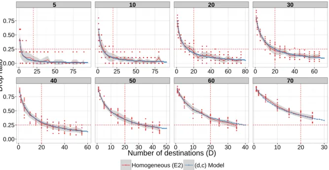
num-ber of sources and destinations. Since all destinations are in-distinguishable, each time we meet one a message is delivered. Figure 5 (on page 6) shows the evolution of the drop ratio when increasing the number of destinations for different values of S such as ⇢ 2 {5%, 10%, 20%, 30%, 40%, 50%, 60%, 70%}. The number of destinations D varies up to the maximum amount
of free nodes on each case, i.e. 1 D < N S. We can see
how adding destinations reduces the drop ratio because of the increase of delivery probability. We see the match between the model and simulated results. We also notice that the variance is lower with a higher number of sources as in the E1 case. This graph allows to define how many nodes are needed in an anycast sensor network to keep the drop ratio bounded. Indeed, we observe that with 20 anycast destinations we can obtain a drop ratio lower than 25% for a network occupancy in between 30% and 40%.
C. Heterogeneity with two classes
In this section we discuss both simulations E3 and E4
with the main results for the two-class (d, c1, c2) model. We
have N = 100 nodes, D = 1 destination, and the rest of nodes
divided in two classes C1 and C2 of same size (N1= 50 and
N2 = 49 respectively). We increase the number of sources
selecting randomly M1 from C1 and M2 from C1 such that
M = M1+ M2. We define 1= 2.5, 2= 200, = 66.6 for
E3 and 01= 10, 02= 100, 0=
0 1+ 02
2 = 55for E4.
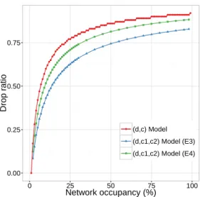
Figure 6a presents the compared model results for three
cases: (d, c) model and (d, c1, c2)for E3 and E4 simulations.
First, we can see that the homogeneous case performs worse than both two-class heterogeneous cases. Recall that the
prob-abilities of the (d, c) model are independent of while in
the (d, c1, c2) model they are not. Indeed, we see how the
assigned values for the E3 case give a lower drop ratio than E4. This is due to the encounter rates defined: on simulation
E3, we have 1 < < 2. This means that nodes in class
C1 meet more frequently than the nodes in C2, and nodes in
C2 meet more frequently a node from C1 than from their own
class. Consequently, messages in the first class will reach the destination more frequently than the ones in the second class, and messages in the second class can also benefit from the transfer opportunities to the first class to be in turn forwarded to the destination. Since messages are being delivered more frequently, we decrease the drop ratio in comparison with the homogeneous case. On contrast, on simulation E4 the drop ratio increases. If we think in terms of interactions between nodes, the total number of pairs is 4950, with ⇠ 1225 pairs per
group. The number of interactions is distributed as C1⇠ 25%,
C2⇠ 25% and 50% for the inter-class interactions. In E4, the
rates are in the same configuration as E3, but with a difference
in the order of magnitude as 0
1< 0 < 02: values 01 and 02
in E4 are closer to a unique value than 1 and 2 in E3.
Hence, more than half of interactions behave similarly in terms of encounter frequency, which explains why E4 is closer to the homogeneous case than E3. We see how the frequency of contacts is key to characterizing the heterogeneity.
Figure 6 shows how the two-class model matches our simulations in both number of drops and drop ratio. In this figure we include the model for both E3 and E4, as well as the simulation results in a 95% confidence interval. Like in
● ● ● ●● ●● ●● ●● ● ●●●● ●●●● ●● ● ●●●●● ●●●●● ● ●●●●●●●●●● ● ●●●●●●●●●● ● ●●●●●●●●●● ● ●●●●●●●●●● ● ●●●●●●●●●● ● ●●●●●●●●●● 0.00 0.25 0.50 0.75 0 25 50 75 100 Network occupancy (%) Drop r atio ● (d,c) Model (d,c1,c2) Model (E3) (d,c1,c2) Model (E4)
(a) Comparison between the (d, c) and the (d, c1, c2)
mod-els. For the (d, c1, c2)model, different ICT parameters are
considered (E3 and E4).
● ● ●● ●● ●● ●● ● ●●●● ●● ●●●● ● ● ● ● ● ● ● ● ● ● ● ● ● ● ● ● ● ● ● ● ●● 0.00 0.25 0.50 0.75 0 25 50 75 100 Network occupancy (%) Drop r atio ● (d,c1,c2) Model (E3) (d,c1,c2) Model (E4) Two class symmetrical (E3) Two class symmetrical (E4)
(b) Results for E3 and E4: we see how close the (d, c1, c2)
model-predicted values and the simulated values are for the symmetrical case.
Figure 6: Drop ratio for two-class simulations E3 and E4.
the homogeneous case, we observe that with less sources we have a bigger variance on the simulated results.
IV. CONCLUSIONS
In this work, we studied the drop ratio for the progression of messages from a set of sources to a set of destinations. Each source emits one message that can be absorbed by any destination. Messages in our study are simply forwarded among nodes to avoid the inclusion of extra copies (replica-tion), which will only increase the probability of drops. We worked with nodes with 1-message buffers to represent the worst case: all nodes are saturated and we want to know how many new messages can be injected (upper bound). Our main contribution is the introduction of a continuous time Markov chain model to characterize the drop of messages under these hypotheses. We introduced two variants: the (d, c) model for
● ● ●● ● ● ●● ● ●● ●●●●● ● ●●● ● ● ●● ● ●●●● ● ● ●●●●●● ●●● ●● ● ● ● ●●●●●● ●● ● ●●● ●●● ● ● ●●● ●● ● ●●● ● ●●●●● ●●● ●● ●●● ● ●●●●● ●●●●●● ●● ● ●● ● ●● ● ● ●● ● ● ● ● ●●●● ● ●● ●● ● ●● ●● ●●●● ●●●●●● ●●● ● ● ● ●● ●●● ● ●● ●●●●●● ●●● ● ● ●●● ●●●●●● ●●●●●● ●●● ●● ●● ● ●●●● ● ● ●●●●●● ●●● ●● ● ● ● ● ● ●● ● ● ● ●● ●● ●● ● ● ● ● ● ● ● ● ● ● ● ● ● ●● ●● ● ● ● ● ● ●● ● ● ● ● ● ● ● ● ● ● ● ● ● ● ● ● ● ● ● ● ● ● ●● ●● ● ●● ●● ● ● ● ● ● ● ● ● ● ● ● ● ●● ● ● ● ● ● ● ● ● ● ● ● ● ● ● ● ● ● ●● ● ● ● ●● ● ● ● ● ● ● ● ● ●● ● ● ● ● ● ● ● ● ● ● ● ● ● ● ● ● ● ● ● ● ● ● ● ● ●● ● ● ●● ● ● ● ● ● ● ● ● ● ● ●● ● ●● ●● ●● ● ●● ●● ● ●● ● ● ● ● ● ●● ●● ●● ● ● ● ● ● ● ● ● ● ● ● ● ● ● ● ● ● ● ● ● ● ● ● ● ● ● ● ● ● ● ● ● ● ● ● ● ● ● ● ● ● ● ● ● ● ● ● ● ● ● ● ● ● ● ● ● ● ● ● ● ● ● ● ● ● ● ● ● ● ●● ● ● ● ● ● ● ● ● ● ● ● ● ● ● ● ● ● ● ● ● ● ● ● ● ● ● ● ● ● ● ● ● ● ● ● ● ● ● ● ● ● ● ● ● ● ● ● ● ● ● ● ● ● ● ● ● ● ● ● ● ● ● ● ● ● ● ● ● ● ● ● ● ● ● ● ● ● ● ● ● ● ● ● ● ● ● ● ● ● ● ● ● ● ● ● ● ● ● ● ● ● ● ● ● ● ● ● ● ● ● ● ● ● ● ● ● ● ● ● ● ● ● ● ● ● ● ● ● ● ● ● ● ● ● ● ● ● ● ● ● ● ● ● ● ● ● ● ● ● ● ● ● ● ● ● ● ● ● ● ● ● ● ● ● ● ● ● ● ● ● ● ● ● ● ● ● ● ● ● ● ● ● ● ● ● ● ● ● ● ● ● ● ● ● ● ● ● ● ● ● ● ● ● ● ● ● ● ● ● ● ● ● ● ● ● ● ● ● ● ● ● ● ● ● ● ● ● ● ● ● ● ● ● ● ● ● ● ● ● ● ● ● ● ● ● ● ● ● ● ● ● ● ● ● ● ● ● ● ● ● ● ● ● ● ● ● ● ● ● ● ● ● ● ● ● ● ● ● ● ● ● ● ● ● ● ● ● ● ● ● ● ● ● ● ● ● ● ● ● ● ● ● ● ● ● ● ● ● ● ● ● ● ● ● ● ● ● ● ● ● ● ● ● ● ● ● ● ● ● ● ● ● ● ● ● ● ● ● ● ● ● ● ● ● ● ● ● ● ● ● ● ● ● ● ● ● ● ● ● ● ● ● ● ● ● ● ● ● ● ● ● ● ● ● ● ● ● ● ● ● ● ● ● ● ● ● ● ● ● ● ● ● ● ● ● ● ● ● ● ● ● ● ● ● ● ● ● ● ● ● ● ● ● ● ● ● ● ● ● ● ● ● ● ● ● ● ● ● ● ● ● ● ● ● ● ● ● ● ● ● ● ● ● ● ● ● ●● ● ● ● ● ● ● ● ● ● ● ● ● ● ● ● ● ● ● ● ● ● ● ● ● ● ● ● ● ● ● ● ● ● ● ● ● ● ● ● ● ● ● ● ● ● ● ● ● ● ● ● ● ● ● ● ● ● ● ● ● ● ● ● ● ● ● ● ● ● ● ● ● ● ● ● ● ● ● ●● ● ● ● ● ● ● ● ● ● ● ● ● ● ● ● ● ● ● ● ● ● ● ● ● ● ● ● ● ● ● ● ● ● ● ●● ● ● ● ● ● ● ● ● ● ● ● ● ● ● ● ● ● ● ● ● ● ● ● ● ● ● ● ● ● ● ● ● ● ● ● ● ● ● ● ● ● ● ● ● ● ● ● ● ● ● ● ● ● ● ● ● ● ● ● ● ● ● ● ● ● ● ● ● ● ● ● ● ● ● ● ● ● ● ● ● ● ● ● ● ● ● 5 10 20 30 40 50 60 70 0.00 0.25 0.50 0.75 0.00 0.25 0.50 0.75 0 25 50 75 0 25 50 75 0 20 40 60 80 0 20 40 60 0 20 40 60 0 10 20 30 40 50 0 10 20 30 40 0 10 20 30 Number of destinations (D) Drop r atio
● Homogeneous (E2) (d,c) Model
Figure 5: Results for E2: each graph represents a fixed network occupancy ⇢. We see how adding destinations decreases the drop ratio as predicted by the model. We see the number of destinations needed to get a 25% drop ratio for each case.
homogeneous contact between nodes and the (d, c1, c2) for
a two-class heterogeneous case. Based on these models, we show the link between the encounter rate among nodes with the drop ratio of forwarded messages: the selection of these rates can impact the message dropping behavior. In specific, we showed that some configurations behave better than the homogeneous case, while others behave close to it. From the model we can extract the trade-off between the number of sources and destinations nodes in order to achieve a desired drop ratio requirement. We performed a DTN simulation to calculate the drop ratio for several scenarios to validate the model. We showed that the outputs of the CTMC model fit to DTN simulation outputs. For future work, we plan to better characterize the behavior of the two-class model by varying encounter frequencies. We will also investigate the cases of larger buffers and full heterogeneity.
ACKNOWLEDGMENTS
The authors would like to thank Patrick S´enac for his ideas to improve this work. This work is partially supported by CONICYT (Becas Chile PhD program).
REFERENCES
[1] K. Fall, “A delay-tolerant network architecture for challenged internets,” ser. ACM SIGCOMM 2003, pp. 27–34.
[2] M. Conti and S. Giordano, “Mobile ad hoc networking: milestones, challenges, and new research directions,” IEEE Communications Mag-azine, vol. 52, no. 1, pp. 85–96, January 2014.
[3] R. Groenevelt, P. Nain, and G. Koole, “The message delay in mobile ad hoc networks,” Performance Evaluation, pp. 210–228, 2005. [4] Z. Haas and T. Small, “A new networking model for biological
appli-cations of ad hoc sensor networks,” IEEE/ACM Trans. on Networking, vol. 14, no. 1, pp. 27–40, 2006.
[5] Y.-K. Ip, W.-C. Lau, and O.-C. Yue, “Performance modeling of epi-demic routing with heterogeneous node types,” in IEEE ICC 2008, pp. 219–224.
[6] A. Hanbali, P. Nain, and E. Altman, “Performance of ad hoc networks with two-hop relay routing and limited packet lifetime,” in IEEE IWQoS 2006, pp. 295–296.
[7] M. Abdulla and R. Simon, “The impact of the mobility model on delay tolerant networking performance analysis,” in ANSS 2007, pp. 177–184. [8] T. Spyropoulos, K. Psounis, and C. Raghavendra, “Efficient routing in intermittently connected mobile networks: The multiple-copy case,” IEEE/ACM Trans. on Networking, 2008.
[9] R. Diana and E. Lochin, “Modelling the delay distribution of binary spray and wait routing protocol,” in IEEE WoWMoM 2012.
[10] X. Zhang, G. Neglia, J. Kurose, and D. Towsley, “Performance mod-eling of epidemic routing,” Computer Networks, vol. 51, no. 10, pp. 2867–2891, 2007.
[11] L. Sassatelli and M. Medard, “Inter-session network coding in delay-tolerant networks under spray-and-wait routing,” in WiOpt 2012. [12] R. Gunasekaran, V. Mahendran, and C. Siva Ram Murthy, “Performance
modeling of delay tolerant network routing via queueing petri nets,” in IEEE WoWMoM 2012.
[13] F. Brauer and C. Castillo-Chavez, “Epidemic models,” in Mathematical Models in Population Biology and Epidemiology, ser. Texts in Applied Mathematics. Springer, 2012, pp. 345–409.
[14] T. Spyropoulos, T. Turletti, and K. Obraczka, “Routing in delay-tolerant networks comprising heterogeneous node populations,” IEEE Trans. on Mobile Computing, vol. 8, no. 8, pp. 1132–1147, 2009.
[15] C. Boldrini, M. Conti, and A. Passarella, “Modelling social-aware forwarding in opportunistic networks,” in Performance Evaluation of Computer and Communication Systems. Milestones and Future Chal-lenges, ser. Lecture Notes in Computer Science. Springer, 2011, vol. 6821, pp. 141–152.
[16] A. Picu, T. Spyropoulos, and T. Hossmann, “An analysis of the information spreading delay in heterogeneous mobility DTNs,” in IEEE WoWMoM 2012.
[17] V. Manam, V. Mahendran, and C. Siva Ram Murthy, “Performance mod-eling of routing in delay-tolerant networks with node heterogeneity,” in COMSNETS 2012, pp. 1–10.
[18] R. Subramanian and F. Fekri, “Throughput analysis of delay tolerant networks with finite buffers,” in IEEE MASS 2008.
![Table I: Previous literature considering finite/infinite buffers. Only [10] characterizes the drop ratio with finite buffers, using ODEs and focusing on homogeneous ICT and epidemic routing.](https://thumb-eu.123doks.com/thumbv2/123doknet/3178895.90731/3.918.120.804.141.258/previous-literature-considering-infinite-characterizes-focusing-homogeneous-epidemic.webp)