Decentralized power systems : reference-frame theory and stability region generation

(1)

Decentralized Power Systems: Reference-Frame

Theory and Stability Region Generation

by

Colm J. O’Rourke

B.E., Energy Systems Engineering

National University of Ireland, Galway (2013)

S.M., Electrical Engineering and Computer Science

Massachusetts Institute of Technology (2015)

Submitted to the Department of Electrical Engineering and Computer

Science

in partial fulfillment of the requirements for the degree of

Doctor of Philosophy in Electrical Engineering and Computer Science

at the

MASSACHUSETTS INSTITUTE OF TECHNOLOGY

May 2020

c

○ Massachusetts Institute of Technology 2020. All rights reserved.

Author . . . .

Department of Electrical Engineering and Computer Science

May 15, 2020

Certified by . . . .

James L. Kirtley

Professor of Electrical Engineering

Thesis Supervisor

Accepted by . . . .

Leslie A. Kolodziejski

Professor of Electrical Engineering and Computer Science

Chair, Department Committee on Graduate Students

(2)

(3)

Decentralized Power Systems: Reference-Frame Theory and

Stability Region Generation

by

Colm J. O’Rourke

Submitted to the Department of Electrical Engineering and Computer Science on May 15, 2020, in partial fulfillment of the

requirements for the degree of

Doctor of Philosophy in Electrical Engineering and Computer Science

Abstract

Electricity provides the foundation for many of today’s technological advances. The desire for energy security, a reduction in carbon dioxide emissions and a diversifica-tion of resources are all motivadiversifica-tions for changes in how electricity is generated and transmitted. Recent alternatives to traditional centralized power-plants include tech-nologies that are decentralized and intermittent, such as solar photovoltaic and wind power. This trend poses considerable challenges in the hardware making up these sys-tems, the software that control and monitor power networks and their mathematical modelling.

This thesis presents a set of contributions that address some of the aforemen-tioned challenges. Firstly, we examine the fundamental theories used in modelling and controlling power systems. We expand previous work on reference-frame theory, by providing an alternative interpretation and derivation of the commonly used Park and Clarke transformations. We present a geometric interpretation that has applica-tions in power quality. Secondly, we introduce a framework for producing regions of stability for power systems using conditional generative adversarial neural networks. This provides transmission and distribution operators with an accurate set of control options even as the system changes significantly.

Thesis Supervisor: James L. Kirtley Title: Professor of Electrical Engineering

(4)

(5)

Acknowledgments

PhD theses are primarily an account and celebration of individual contributions to a field. In reality, we all learn from each other and no work is done in strict isolation. With this in mind, I have a few groups of people I would like to acknowledge in this work.

First and foremost my sincere thanks to my thesis supervisor Professor Kirtley. His patience and support was tremendously helpful in completing this research. He was always open to working on new problems including those not traditional to his research background. He gave me the freedom to grow and mature as a researcher and I am grateful to have had him as my advisor. I also wish to thank my committee members Professors Lang and Peng, for their helpful guidance on how to improve my work. Professor Lang took the time to explain answers to any questions I had over the years. I learned a lot from these discussions and I am grateful I had that opportunity to learn from him. Professor Peng made the collaboration happen between MIT and the National University of Singapore (NUS). It was one of the highlights of my PhD experience. He was always very welcoming to me whenever I visited NUS or the Masdar Institute in Abu Dhabi and I express my gratitude for this.

Part I of this thesis arose from a collaboration with Mohammad Qasim and Matthew Overlin. I offer my sincere gratitude to both of them for helping out with this - in particular, they both helped enormously in addressing reviewers’ comments when we were trying to get that paper published.

Part II of this thesis stems from a collaboration between MIT and NUS. I wish to thank both Gurupraanesh Raman and Jerry Lu for the enormous amount of work put into this project. I wish to acknowledge Jerry for all of the hours he spent tuning hyperparameters and working on making our models better in general. I also want to thank Praanesh for developing this framework with me and for all the late nights, early mornings and brainstorming we did. I wish to also thank Krishan Kant who helped with the damping case study.

(6)

and Krishan Kant for making work such a fun place to be. I learned a lot from each of them, both technical and about life in general. I couldn’t imagine doing research without having them all to discuss ideas with. I wish to thank the rest of Professor Kirtley’s group and the students and staff at LEES in general, past and present. I am grateful to be in such a positive lab environment where there is a culture of helping each other out. There are too many names to mention here so at the risk of forgetting someone I express gratitude for them all. I am thankful for all of the staff at the EECS Headquarters. In particular, I wish to thank Janet Fisher, Alicia Duarte, Claire Benoit and Leslie Kolodziejski.

I am thankful for all of the teachers I had through the years. After 24 years in education, that number is probably fairly high. I acknowledge all of the staff I was fortunate to learn from at Walsh Island national school, Coláiste Íosagáin in Portarlington and at the National University of Ireland, Galway. In particular, I acknowledge my secondary school maths teacher Mr. Aughney, my thermodynamics lecturer Nathan Quinlan, as well as Rory Monaghan and Ger Hurley who both en-couraged me to apply to MIT. I also acknowledge mentors who offered help and advice whenever I needed it: Frankie O’Sullivan, Ronán McGovern and Kevin O’Keeffe.

I would like to thank everyone involved in the MIT Rowing Club and the MIT Hyperloop team. A special thanks to my bandmates and great friends Gus Lonergan and Pavel Chvykov for filling my life with music. Each of these groups were a huge part of my experience and I have many memories as a result. I am grateful for all of the friends I made at MIT and in Boston in general. I would like to thank them all for making this feel like home. In particular I wish to thank the MIT Irish society and the general Irish community here in Boston for all of the laughs and good times. I would like to thank my roommates over the years for making my home a place I was happy to return to after a long day’s work. Again, there are too many names to mention with each of these groups so I acknowledge all of them and I look forward to making new memories with them all in the future.

Finally, and most importantly, I wish to thank my family and extended family at home in Ireland and abroad. In particular, I wish to thank my parents Mary and

(7)

Michael and my siblings Evelyn, Tadhg, Matthew and Michael. They were always there to support me and growing up I felt confident I could become whatever I wanted thanks to them. I have a great family community and I am grateful and lucky to have them all. Go raibh maith agaibh go léir.

(8)

(9)

List of Figures

2-1 Relationships between Transformations . . . 21

2-2 Transformations Applied to Waveforms . . . 22

2-3 Clarke’s Derivation . . . 23

2-4 Synchronous Machine Cross-Section . . . 24

2-5 Park’s Derivation . . . 25

2-6 Geometric Interpretation of the Clarke and Park Transformations. . . 30

2-7 Phasor vs. Cartesian Representation . . . 34

2-8 Locus Diagram for Balanced System . . . 35

3-1 Geometric Power-Invariant Clarke Transformation . . . 38

3-2 Geometric Power-Invariant Inverse Clarke Transformation Derivation 40 3-3 Standard (Aamplitude-Invariant) Clarke Transformation . . . 42

3-4 Geometric Standard (amplitude-invariant) Inverse Clarke Derivation . 45 3-5 𝛼𝛽0 to 𝑑𝑞0 Transformation . . . 45

3-6 Geometric 𝛼𝛽0 to 𝑑𝑞0 Derivation . . . 48

3-7 Standard (Amplitude-Invariant) Park Transformation . . . 50

3-8 Geometric Standard (Amplitude-Invariant) Inverse Park Derivation . 53 3-9 Geometric Interpretation of Unbalance . . . 54

3-10 Geometric Interpretation of Harmonics . . . 56

3-11 Locus Diagram with Harmonics . . . 56

4-1 cGANs-Based Framework for Stability Region Generation . . . 63

(12)

5-1 Case Study for Stability Region Generation . . . 72

5-2 Accuracy and Coverage Results . . . 75

5-3 Sample Stability Regions Generated using cGANs . . . 76

5-4 Operating Point Selection within Stability Regions . . . 76

(13)

List of Tables

4.1 cGANs Hyperparameters used in Case Study . . . 67

5.1 Training and Testing Cases used for cGANs . . . 73

B.1 Summary of Transformations . . . 86

(14)

(15)

Chapter 1 Introduction

Electricity provides the foundation for many of today’s technological advances. The desire for energy security, a reduction in carbon dioxide emissions and a diversifica-tion of resources are all motivadiversifica-tions for changes in how electricity is generated and transmitted. Recent alternatives to traditional centralized power-plants include tech-nologies that are decentralized and intermittent, such as solar photovoltaic and wind power. This trend poses considerable challenges in the hardware making up these sys-tems, the software that control and monitor power networks and their mathematical modelling.

Traditional centralized power systems consist of sources in the form of coal, gas, nuclear and hydro power plants. The synchronous machine is at the heart of the mechanical to electrical energy conversion process, for each of these centralized power plants. As more renewables such as wind and solar penetrate the electricity grid, the percentage of non-inertial generation on the system increases. Many of these renewable technologies use DC to AC converters at their interface, meaning that the synchronous machine may not dominate power systems in the same way as it has in the past. Although the generation of electricity increasingly relies on a mix of tech-nologies, these technologies use common mathematical tools (such as transformations) that were derived with respect to a specific application. For example the Park trans-formation was derived to help in the modelling of synchronous generators, yet this transform finds uses in numerous other fields including inverter control. The 𝑑 and 𝑞

(16)

axes have physical meaning when referring to a synchronous machine, yet three-phase inverters often make use of the Park transformation. This motivates an alternative interpretation of reference-frames which is agnostic to a specific application. This is the first area of contributions in this thesis.

The second area of contributions focuses on the implications of decentralized power systems on the system operator. Decentralization can cause increased variability in the system, as the number of renewable energy sources connected to the grid increase. System operators must maintain system stability in spite of system changes such as faults, fluctuating supply and demand and alternate network topologies. In order to make dynamic decisions to maintain stability, the system operator first needs to have a better sense of the system health. This motivates a stability region generation tool that operators can use to view how stability regions are changing in real-time. This is the second area of contributions in this work.

1.1 Thesis Structure

This thesis outlines two solutions regarding the decentralization of power systems: Ge-ometric Reference-Frame Theory and Stability Region Generation. As the technical details of these solutions are quite distinct, they are separated into Part I (geomet-ric reference-frame theory) and Part II (stability region determination). Despite this distinct structure, Part I and Part II make up two solutions to a single application: decentralized generation in power systems.

The author directs the reader to the beginning chapter of each section for a lit-erature review for each of the problems, as well as a list of contributions made using the proposed approaches.

(17)

Part I

A Geometric Interpretation of

Reference-Frames

(18)

(19)

Chapter 2 Reference-Frame Theory

This chapter provides an overview of Part I of this thesis. The objective of this thesis is to address challenges associated with the decentralization of generation in power systems. Traditional centralised power systems have been dominated by the synchronous machine for the past 100 years. An increased proportion of renewables often leads to a higher proportion of inverters interfacing with the electricity network. This is because many renewable technologies such as solar photovoltaic and wind-farms require DC to AC converters at their interface. As the number of inverters increases, the synchronous machine may not dominate power system generation as it has done in the past. Transformations such as the Clarke transformation were derived with the intention to analyse specific problems such as unbalanced three-phase faults, yet somehow find uses in numerous other applications including three-phase inverter control. This motivates an alternative interpretation of reference-frames which is agnostic to a specific application. This problem is the focus of Part I of this thesis, which provides a solution in the form of a geometric interpretation of reference-frame theory [1].

2.1 Overview and Motivation

A reader familiar with the commonly used Clarke and Park transformations may wonder as to why one would want to investigate them further. One could argue

(20)

that the transformations already exist and therefore what benefit is there in addi-tional research? The motivation to contribute to reference-frame theory stem from two main observations: (i) the Clarke and Park transformations were derived with respect to specific applications in mind, yet somehow both find uses in many appli-cations beyond their original intention and (ii) signals with unbalance and harmonics have interesting properties when observed in the 𝑑𝑞0 frame. Beyond this, the author believes there is value in a more general framework to understand these transforma-tions, as this can allow one to gain a deeper understanding and intuition. One could also compare this to the analogy of music versus music theory. Music has existed since the early days of humankind - long before music theory was developed. Yet, the theoretical framework for music somehow makes it more rich and interesting for some people. Similarly, the Clarke and Park transformations already exist, but perhaps the geometric interpretation provided here adds depth to the field of reference-frame theory.

Transformations between 𝑎𝑏𝑐 and 𝑑𝑞0 reference-frames were originally used to

assist in electrical machine analysis and modelling [2]. Currently, 𝑑𝑞0 based models are used in a wide variety of applications including: modelling and control of electric machines and drives [2, 3], multimachine modelling [4], multi-inverter modelling [5], microgrid simulation [6–8], phase-locked loops (PLLs) [9] and active power filters [10]. In many of these examples, the dq components no longer refer to the direct and quadrature axes of a machine. This motivates an alternative interpretation of reference-frames that is detached from any specific technology or application. This thesis provides one such alternative perspective which is referred to as the “geometric interpretation”.

2.2 Previous Work

Considering the wealth of literature available on the subject of reference frames, it is essential that the contributions of this work are positioned in the context of previous work. To this end, the history of these transformations must first be studied,

(21)

taking care to cite the most notable references. Krause’s arbitrary reference-frame and how this perspective relates to each transformation is reviewed. Following this, the geometric approach to deriving the Clarke and Park transformation matrices is presented. The contributions of this thesis are distinguished from previous work, and the advantages and disadvantages of the geometric approach are discussed.

2.2.1 Review of the Clarke and Park Transformations

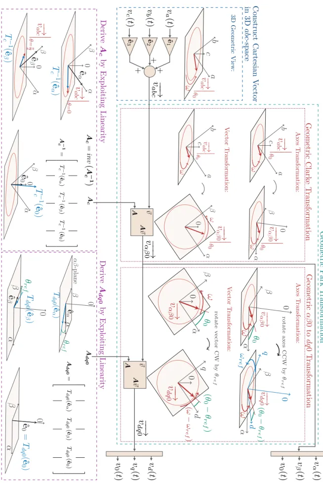
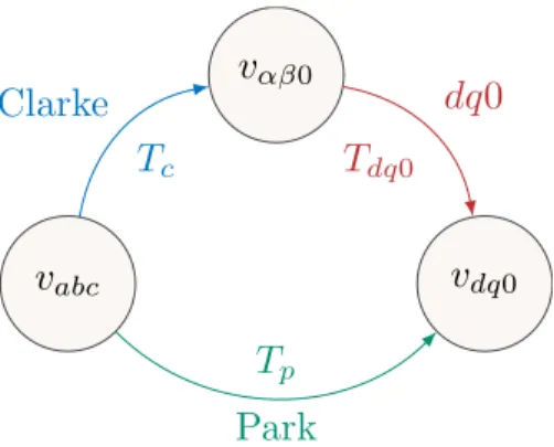
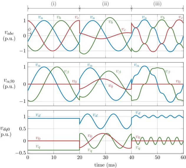
Fig. 2-1 provides an overview of the transformations. The Clarke transformation con-verts three-phase 𝑎𝑏𝑐 quantities to 𝛼𝛽0 (ie stationary 𝑑𝑞0). The Park transformation converts 𝑎𝑏𝑐 quantities to 𝑑𝑞0 and can be thought of as applying the Clarke trans-formation first, followed by the 𝛼𝛽0 to 𝑑𝑞0 transformation. Here the latter is simply referred to as the “𝑑𝑞0 transformation” for simplicity of subscript notation. Later it will be discussed how this corresponds to the “frame-to-frame-transformation” as described in [2]. vαβ0 vabc vdq0 Park Tp Clarke Tc dq0 Tdq0

Figure 2-1: Relationships between the Park and Clarke transformations. Note that the term “𝑑𝑞0 transform” as defined in this thesis refers to a transformation from 𝛼𝛽0 to𝑑𝑞0 and is therefore not equivalent to the Park transformation.

Fig. 2-2 shows the affect of applying the standard Clarke and Park transformations under three different conditions: (i) Balanced voltages result in equal magnitudes for 𝑣𝛼 and 𝑣𝛽 and constant values of 𝑣𝑑 and 𝑣𝑞. (ii) Unbalanced voltages result in unequal magnitudes for 𝑣𝛼 and 𝑣𝛽 and time-varying 𝑣𝑑 and 𝑣𝑞 at the 2nd harmonic. 𝑣0 is a zero-sequence component at the fundamental and is always identical in both transformations.

(22)

−1 0 1 va vb vc va vb vc va vb vc φ

v

abc (p.u.) −1 0 1 vα vβ v0 vα vβ v0 vα vβ v0

v

αβ0 (p.u.) 0 10 20 30 40 50 60 −0.5 0 0.5 1 vd vq v0 vd vq v0 vd vq v0 time (ms)

v

dq0 (p.u.)

(i) (ii) (iii)

Figure 2-2: Clarke and Park transformations applied to three-phase 50 Hz voltages under three conditions: (i) balanced fundamental frequency with a phase shift (ii) unbalanced fundamental (iii) balanced with harmonics (1st_{, 5}th_{, 7}th_).

Condition (iii) in Fig. 2-2 illustrates the affect of harmonics. Each phase voltage includes fundamental, 5th _{and 7}th _{harmonics, with balanced voltages at each} har-monic. These particular harmonics appear as a 6th harmonic in 𝑣𝑑 and 𝑣𝑞. There is no zero-sequence component for these particular harmonics. The voltage𝑣𝛼 is equiv-alent to𝑣𝑎; and 𝑣𝛽 has a different harmonic profile to 𝑣𝑏 due to a180∘ phase-shift on its positive sequence components. In Section 3.3, each of the conditions (i), (ii) and (iii) in Fig. 2-2 are explained using the geometric interpretation.

(23)

History of the Clarke Transformation

In 1912, Stokvis introduced the concept of decomposing unbalanced three-phase sig-nals into positive and negative sequence [11]. His example in [11, 12] describes a three-phase generator with a floating neutral node, and how unbalanced currents in such a system can be decomposed into “synchronous” and “inverse” currents (ie positive and negative sequence currents). Fortescue built on the work of Stokvis by introducing zero-sequence and generalising the decomposition for 𝑁 phases in [13].

In the 1930s, Clarke made a series of modifications to symmetrical components [14, 15]. These modifications simplified the calculations for certain classes of unbalanced

three-phase problems [15, 16]. The 𝛼, 𝛽 and 0 components were one set of these

innovations [15], and were particularly useful as they did not require the 𝑎 operator (1 120∘_{) or complex numbers. Although Clarke’s derivation in Fig. 2-3 requires both} the𝑎 operator and a multiplication by 𝑗, the resulting transformation matrix does not contain any complex numbers, unlike the symmetrical components transformation.

+ 0

abc

++ + va(t) vb(t) vc(t) v↵(t) v (t) v0(t) V0 V Vc Vb Va V+ V V↵ V0 Time Domain to Phasor Domain Symmetrical Components Phasor Domain to Time Domain V _{! v(t)} v(t)_{! V} j

Figure 2-3: An illustration of the Clarke transformation as derived in [15].

Fig. 2-3 provides an illustration of the derivation developed by Clarke. The 𝛼 component is defined as the sum of the positive and negative sequence voltage phasors, whereas the 𝛽 component is the difference between positive and negative sequence phasors, times_{−𝑗. Clarke’s 0 component is equivalent to the zero sequence as defined} by symmetrical components. For a comprehensive discussion of Clarke’s derivation, the author refers the reader to [15].

(24)

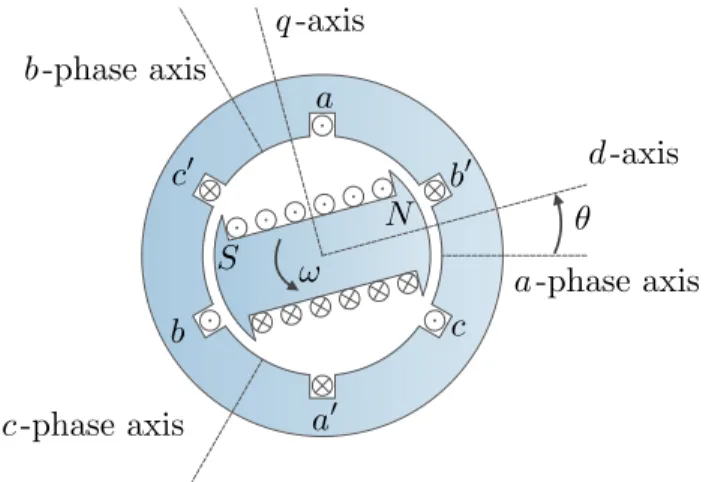
c -phase axis a -phase axis b -phase axis d -axis q -axis ✓ N S a a0 b b0 c c0 !

Figure 2-4: Cross-section of a synchronous machine

History of the Park Transformation

In 1899, Blondel developed the two-reactance method to study the behaviour of syn-chronous machines [17, 18]. This method resolves the armature fluxes in a salient machine along the two axes of symmetry: the direct and quadrature axes. Fig. 2-4 shows the physical definitions of the direct and quadrature axes.

During the 1920s, Park generalised Blondel’s Two-Reaction Theory of Synchronous Machines [17–20]. This method resolves the armature fluxes in a salient machine along the two axes of symmetry: the direct and quadrature axes. Fig. 2-4 shows the phys-ical definitions of the direct and quadrature axes. This thesis uses the convention that the 𝑑-axis points in the direction of the rotor flux. Park’s derivation shown in Fig. 2-5 actually defines the inverse transformation: 𝑑𝑞0 to 𝑎𝑏𝑐. The steps are as follows: Firstly, assume that armature flux linkages can be resolved into two compo-nents: directly in phase with the rotor (𝜆𝑑) and in quadrature with the rotor (𝜆𝑞). Secondly, project the 𝑑 and 𝑞-axes flux linkages onto the three coplanar 𝑎𝑏𝑐 magnetic

axes. Finally, add a zero sequence component (𝜆0) to each phase. The reader is

referred to [19] for a more complete description of Park’s derivation.

2.2.2 Review of the Arbitrary Reference-Frame

A “reference-frame” refers to a set of𝑑𝑞0 axes rotating at a particular speed 𝜔 (which may be zero). In the 1920s Park chose to rotate his 𝑑𝑞0 axes as defined in [19] at

(25)

b(t) + + a(t) + + + + c(t) 0(t) d(t) q(t)

Stator Flux Linkages

dcos ✓ qsin ✓ dcos ✓ ✓ + 2⇡ 3 ◆ qsin ✓ ✓ + 2⇡ 3 ◆ dcos ✓ ✓ 2⇡ 3 ◆ qsin ✓ ✓ 2⇡ 3 ◆ d q b c a d q d q d q d q

Project d and q onto abc axes w.r.t. dq frame

Figure 2-5: An illustration of the Park transformation as derived in [19]

the rotor speed of a synchronous machine 𝜔𝑟 (because that speed eliminates time-varying inductance in synchronous machine analysis). During the 1930s-1950s others [21–23] used alternative reference speeds for their 𝑑𝑞0 axes, to assist in the analysis of induction machines. Eliminating time-varying inductance in addition to achieving a diagonalised inductance matrix were primary objectives [2].

In 1965, Krause described in [24] that all of the different reference-frames used in [15, 19, 21–23] are specific applications of the “arbitrary reference-frame”. They all refer to𝑑𝑞0 axes that rotate at a specified 𝜔. A list of commonly used reference-frame speeds are given below [2]:

∙ 𝜔. The 𝑑𝑞0 axes rotate at an arbitrary speed. [24]. ∙ 𝜔 = 𝜔𝑟. The 𝑑𝑞0 axes rotate at the rotor speed [19]. ∙ 𝜔 = 𝜔𝑒. The𝑑𝑞0 axes rotate at the synchronous speed.

∙ 𝜔 = 0. The 𝑑𝑞0 axes are stationary (Clarke transformation).

All of the reference-frames listed can be described by Park’s transformation ma-trix, except that each uses a different rotation speed 𝜔 for the 𝑑𝑞0 axes. The reader is referred to [2] for an extensive discussion of the various reference-frames.

One of the goals of this work is to provide an alternative derivation of Park’s transformation matrix, which describes all of the listed reference-frames (when the

(26)

appropriate 𝜔 is inserted into this matrix). Therefore, a general approach is taken here and an arbitrary reference speed 𝜔 is considered when referring to Park’s trans-formation matrix. This matrix is still referred to as “Park’s transtrans-formation”, even though the reference speed is not limited to be that of the rotor 𝜔𝑟. One is free to choose any reference speed they wish.

2.3 Contributions to Reference-Frame Theory

The contributions of this thesis in the area of reference-frame theory are summarised below. The remainder of this section elaborates on these points:

1. Previous approaches to deriving the matrices describing the Park and Clarke transformations are grouped into two approaches. This work presents a third approach to deriving the Clarke and Park transformation matrices: a geometric approach.

2. The “locus diagram” of a three-phase quantity is introduced along with demon-strations of how this locus changes in the presence of unbalance and harmonics.

The first contribution is to provide an alternative approach to derive the Park and Clarke transformations. Previous work on deriving these transformation matrices follows one of two approaches:

(i) The Clarke transformation matrix is derived from symmetrical components [15] as shown in Fig. 2-3. The Park transformation matrix can be subsequently derived using a rotation matrix such as Eq. (3.17).

(ii) The Park transformation matrix is derived trigonometrically by interpreting the transformation as a rotation in the plane of the cross-section of a machine. The 𝑎𝑏𝑐 axes are coplanar stationary axes that lie 120∘ _{apart and}_{𝑑𝑞 quantities}

can be projected onto the 𝑎𝑏𝑐 axes in a manner shown in Fig. 2-5. A third

transformation variable is introduced to satisfy the change of variables. This is chosen to be the zero component, which is added separately. Many authors

(27)

trigonometrically project in the opposite manner: from 𝑎𝑏𝑐 to 𝑑𝑞 and are thus required to specify scaling factors 𝑘𝑑 and 𝑘𝑞, normally equal to either 2/3 or √︀

2/3: see [25]. These projections describe the approach taken by the majority of authors such as [2, 19, 21–28]. The Clarke transformation matrix can then

be derived trivially by setting 𝜔 = 0 in Park’s transformation matrix. One

should note that the coplanar 𝑎𝑏𝑐 axes are usually considered to have a physical meaning relating to the magnetic axes in the cross-section of a machine as in Fig. 2-4, but this physical interpretation of the 𝑎𝑏𝑐 axes is not necessary to derive the matrix [2].

This thesis section presents a third approach to deriving the Clarke and Park transformation matrices: a geometric interpretation. This geometric approach uses the Cartesian representation: three-phase quantities are represented by vectors in R3_{, where each orthogonal component of the vector corresponds to the instantaneous} value of one of the three phases. The first appearance of the Cartesian representa-tion applied to three-phase quantities was given by Lipo in [29]. Other work that uses this representation includes [30, 31]. More recently, Montanari and Gole use a three-dimensional perspective to introduce a new transformation termed the “ 𝑚𝑛𝑜-transform” [32]. The 𝑚𝑛𝑜-transformation assists in the calculation of instantaneous real and reactive power for systems containing four-wire inverters. This enables the mitigation of power oscillations that normally occur when such systems are unbal-anced [32]. Although others have utilised the Cartesian representation in [29–32], this work is unique as the representation is used to derive the matrices describing the Clarke and Park transformations.

The geometric approach is explained step-by-step in Section 3.1 and Section 3.2. A summary of the derivations provided by the geometric view is given by Fig. 2-6. Each transformation is interpreted as a combination of vector rotation and scaling in R3_{. The} _{𝑎𝑏𝑐 axes are orthogonal stationary axes that lie 90}∘ _{apart and have basis} vectors that span R3. The linearity property of matrix transformations is exploited, and each transformation matrix can be derived by observing how each transformation affects the orthonormal basis vectors of the vector space.

(28)

The geometric approach has many advantages when compared to the two tradi-tional approaches listed previously. These include:

∙ When trigonometrically deriving the Park transformation such as in Fig. 2-5, zero-sequence components are treated separately in the derivation. The 𝑑 and 𝑞 components are found from a projection operation whereas the 0 components

are added separately. The geometric approach finds all 𝑑𝑞0 components in a

unified manner via Eq. (2.5).

∙ The previous approaches interpret the Clarke transformation as either a manip-ulation of symmetrical components as in Fig. 2-3, or as a specialised case of the arbitrary reference-frame with stationary 𝑑𝑞0 axes [2]. The geometric approach interprets the power-invariant Clarke transformation as a single rotation inR3, which some readers may find to be a simpler explanation (see Fig. 3-1). The standard (amplitude-invariant) Clarke transformation is shown in Fig. 3-3 to be a combination of rotation and scaling in R3.

∙ Similarly, previous approaches interpret the Park transformation as either a manipulation of symmetrical components [15] combined with a rotation matrix, or as a projection onto coplanar 𝑎𝑏𝑐 axes [19]. The geometric approach inter-prets the power-invariant Park transformation as two consecutive rotations in R3_{, which some readers may find to be more intuitive (see Fig. 2-6). The} stan-dard Park transformation is interpreted as first applying the stanstan-dard Clarke transform (rotation and scaling) followed by a pure rotation in R3 given by Fig. 3-5.

∙ The orthogonality (𝐴| _{= 𝐴}−1_{) of the power-invariant forms of both} transfor-mations can be easily seen from all three approaches via matrix manipulation. The geometric interpretation illustrates this orthogonal property: orthogonal transformations preserve vector length and can thus be visualised as pure rota-tions inR3 [33].

(29)

approaches include:

∙ The geometric derivation is more involved. This can be seen by comparing Fig. 2-6 to the two traditional approaches illustrated by Fig. 2-3 and Fig. 2-5.

∙ The diagrams required to explain the geometric view are more complex to draw as they are three-dimensional.

The second contribution involves the “locus diagram” of a three-phase quantity and how this locus changes in the presence of unbalance and harmonics. This contribution consists of the following:

∙ In Section 2.5.1 it is shown that for balanced systems, the locus corresponds to a circle inR3. Eq. (2.13) is used to show that this circle has a radius of 𝑉√︀3/2 where 𝑉 is the voltage magnitude on each phase.

∙ In Section 3.3 the locus diagram is extended to cases of harmonics and unbal-ance. Systems with purely positive and negative sequence will have a locus that lies within the𝛼𝛽-plane. The locus of a zero-sequence component is a line segment perpendicular to the 𝛼𝛽-plane.

∙ It is shown that a single locus diagram can fully represent a three-phase quantity containing harmonics in Fig. 3-11. This is not possible using a single phasor diagram.

2.4 Review of Linear Transformations

Transformations are functions that operate on vectors. This section derives a basic method to finding a unique matrix 𝐴 that fully describes a linear transformation 𝑇 : R𝑛_{→ R}𝑚_.

Any vector ⃗𝑣 ∈ R𝑛 _{can be written as a linear combination of the standard basis} unit vectors _{ê1, ê2, . . . , ê𝑛}.

(30)

ê 1 ê 2 ê 3 Ax es T ran sf or m at ion : V ec tor T ran sf or m at ion : 3D G eom et ric Vi ew : V ec tor T ran sf or m at ion : De riv e A dq 0 b y E x p loi tin g Li n ear it y A dq 0 A c De riv e A c b y E x p loi tin g Li n ear it y ~v A ~v A Ax es T ran sf or m at ion : in 3D abc -s p ac e C on st ru ct C ar te sian V ec tor G eom et ric P ar k T ran sf or m at ion G eom et ric C lar k e T ran sf or m at ion G eom et ric ↵ 0t o dq 0 T ran sf or m at ion ~v A ~v A A dq 0 = 2 6 6 6 4 T dq 0 (ê ↵ ) T dq 0 (ê ) T dq 0 (ê 0 ) 3 7 7 7 5 A c = inv A 1 c

!v

abc

!

v

↵ 0

!v

dq 0 v a (t ) v b (t ) v c (t ) v d (t ) v q (t ) v 0 (t ) v 0 (t ) v (t ) v ↵ (t ) ↵ 0 ê 0 = T dq 0 (ê 0₎ + + + ↵ 0 !v ab c ✓=0 ê ↵ T 1 c (ê ↵ ) ↵ 0 !v ab c ✓= ⇡ 2 ê T 1 c (ê ) ↵ T 1 c (ê 0₎ 0 ê 0 ↵ -p lan e ↵ 0 ✓ re f ê ↵ T dq 0 (ê ↵₎ ↵ 0 ✓ re f ê T dq 0 (ê ) A 1 c = 2 6 6 6 4 T 1 c (ê ↵ ) T 1 c (ê ) T 1 c (ê 0 ) 3 7 7 7 5 a b c !v ab c ✓ 0 ! a b c ↵ 0 !v ab c ✓ 0 !v ↵ 0 ✓ 0 ! ! a b c ↵ 0 !v abc ✓ 0 !v ↵ 0 ✓ 0 ! ! ↵ 0 d q 0

!v

dq 0 ✓ 0 (✓ 0 ✓ r ef )

!v

↵ 0

!

(! ! r ef ) rotate v e c tor CW b y ✓ r ef ↵ 0 ↵ d q 0 ! v ↵ 0 !v dq 0 ✓ 0 (✓ 0 ✓ r ef )

!

! r ef rotate axe s CCW b y ✓ r ef Figure 2-6: Geometric in terp re tation of the Clark e and P ark transformations.

(31)

To find 𝑇 (⃗𝑣)_{∈ R}𝑚 _{the linear transformation} _{𝑇 is applied to both sides of equation} 2.1:

𝑇 (⃗𝑣) = 𝑇 (𝑣1^e1+ 𝑣2e^2+ . . . + 𝑣𝑛^e𝑛) (2.2) One can rewrite 𝑇 (⃗𝑣) by imposing the additivity and homogeneity constraints of linearity:

𝑇 (⃗𝑣) = 𝑣1𝑇 (ê1) + 𝑣2𝑇 (ê2) + . . . + 𝑣𝑛𝑇 (ê𝑛) (2.3) 𝑇 (⃗𝑣) in equation 2.3 is now expressed in terms of transformed standard basis vectors scaled by the components of⃗𝑣. Such a linear combination of column vectors can always be written as a matrix-vector product:

𝑇 (⃗𝑣) = ⎡ ⎢ ⎢ ⎢ ⎣ 𝑇 (ê1) 𝑇 (ê2) . . . 𝑇 (ê𝑛) ⎤ ⎥ ⎥ ⎥ ⎦ ⎡ ⎢ ⎢ ⎢ ⎢ ⎢ ⎢ ⎣ 𝑣1 𝑣2 .. . 𝑣𝑛 ⎤ ⎥ ⎥ ⎥ ⎥ ⎥ ⎥ ⎦ 𝑇 (⃗𝑣) = 𝐴⃗𝑣 (2.4)

Eq. (2.4) says that any linear transformation 𝑇 : R𝑛_{→ R}𝑚 _{can be expressed as a} matrix-vector product 𝐴⃗𝑣. 𝐴 = ⎡ ⎢ ⎢ ⎢ ⎣ 𝑇 (ê1) 𝑇 (ê2) . . . 𝑇 (ê𝑛) ⎤ ⎥ ⎥ ⎥ ⎦ (2.5)

Eq. (2.5) describes a technique to determine the𝑚_{× 𝑛 matrix 𝐴, that corresponds} to the linear transformation𝑇 : R𝑛_{→ R}𝑚_{. One can construct}_{𝐴 by applying the linear} transformation to each of the basis vectors of R𝑛. Eq. (2.5) is used in this thesis to geometrically derive the Park and Clarke transformation matrices𝐴𝑃 and 𝐴𝐶.

(32)

2.5 Cartesian Representation of Three-Phase

Volt-ages

Three-phase quantities such as voltages, currents and flux linkages are often expressed using phasor notation. This section introduces the Cartesian representation and com-pares it with phasor notation.

Phasor Representation

Eq. (2.6) is an example of a set of three-phase voltages with no harmonics. For now these voltages may or may not be balanced, where “balanced” would require 𝜑𝑎 = 𝜑𝑏 = 𝜑𝑐= 0 and 𝑉𝑎= 𝑉𝑏 = 𝑉𝑐. ⎧ ⎪ ⎪ ⎪ ⎪ ⎪ ⎨ ⎪ ⎪ ⎪ ⎪ ⎪ ⎩ 𝑣𝑎(𝑡) = 𝑉𝑎cos (𝜔𝑡 + 𝜑𝑎) 𝑣𝑏(𝑡) = 𝑉𝑏cos (𝜔𝑡₋ 2𝜋 3 + 𝜑𝑏) 𝑣𝑐(𝑡) = 𝑉𝑐cos (𝜔𝑡 + 2𝜋 3 + 𝜑𝑐) (2.6)

Each of the three sinusoidal voltages in Eq. (2.6) can be represented by a unique phasor. Phasor notation is the use of a single complex known as a phasor to store

the two parameters of magnitude 𝑉 and phase 𝜑. The magnitude of the phasor 𝑉𝑖

represents the RMS value of 𝑣𝑖(𝑡) and the phase 𝜑𝑖 corresponds to the angle of the voltage𝑣𝑖(𝑡).

Note that the expression for each sinusoidal voltage in Eq. (2.6) is actually defined

by three parameters: voltage magnitude 𝑉𝑖, phase 𝜑𝑖 and frequency 𝜔. A known

frequency must be assumed, which is one limitation of the phasor representation. In addition, the phasor representation cannot be used to represent signals containing more than one frequency component, such as signals with harmonics.

Eq. (2.7) expresses the voltages in Eq. (2.6) as three phasors 𝑉𝑎, 𝑉𝑏 and 𝑉𝑐. These three phasors can be drawn on a single complex plane in a phasor diagram. Fig. 2-7a

(33)

draws a balanced case. _⎧ ⎪ ⎪ ⎪ ⎪ ⎪ ⎪ ⎨ ⎪ ⎪ ⎪ ⎪ ⎪ ⎪ ⎩ 𝑉𝑎 = √1 2𝑉𝑎𝑒 𝑗𝜑𝑎 𝑉𝑏 = √1₂𝑉𝑏𝑒𝑗(− 2𝜋 3 +𝜑𝑏) 𝑉𝑐 = √1 2𝑉𝑐𝑒 𝑗(2𝜋 3 +𝜑𝑐) (2.7)

Each voltage phasor in Eq. (2.7) can be converted back to a function of time using Euler’s relation as shown in Eq. (2.8).

𝑣𝑖(𝑡) =√2 ℜ{𝑉𝑖𝑒𝑗𝜔𝑡_} _(2.8)

Cartesian Representation

The notation −→𝑣𝑎𝑏𝑐is used to signify the Cartesian representation of a set of three-phase voltages. Previous work that uses the Cartesian representation applied to three phase quantities includes: [29–32]. −→𝑣𝑎𝑏𝑐 is a single vector in R3 and has three components corresponding to three orthogonal 𝑎𝑏𝑐 axes:

−→

𝑣𝑎𝑏𝑐 = 𝑣𝑎ê𝑎+ 𝑣𝑏ê𝑏 + 𝑣𝑐ê𝑐 (2.9)

The components of Eq. (2.9) vary with time. Thus −→𝑣𝑎𝑏𝑐 is a vector that moves in R3 over time as seen in Eq. (2.10):

−→ 𝑣𝑎𝑏𝑐(𝑡) = ⎡ ⎢ ⎢ ⎢ ⎢ ⎣ 𝑣𝑎(𝑡) 𝑣𝑏(𝑡) 𝑣𝑐(𝑡) ⎤ ⎥ ⎥ ⎥ ⎥ ⎦= ⎡ ⎢ ⎢ ⎢ ⎢ ⎣ 𝑉𝑎cos (𝜔𝑡 + 𝜑𝑎) 𝑉𝑏cos (𝜔𝑡− 2𝜋 3 + 𝜑𝑏) 𝑉𝑐cos (𝜔𝑡 + 2𝜋₃ + 𝜑𝑐) ⎤ ⎥ ⎥ ⎥ ⎥ ⎦ (2.10)

Fig. 2-7b plots −→𝑣𝑎𝑏𝑐(𝑡) at a particular instance in time 𝑡1. It will be seen later that the locus traced out by −→𝑣𝑎𝑏𝑐(𝑡) over one period is of particular interest.

Fig. 2-7 compares the phasor and Cartesian representations for a three-phase system.

(34)

Re

Im

V

a

V

b

V

c a ab-plane

a

b

c

−−→

v

abc

t1 b

Figure 2-7: Three-phase voltage representations: (a) Phasor representation (b) Cartesian representation at time𝑡1.

– C vector space with two axes 𝑅𝑒 and 𝐼𝑚.

– Three complex numbers (phasors)𝑉𝑎, 𝑉𝑏and𝑉𝑐that do not vary with time. ∙ Cartesian Representation:

– R3 vector space with three orthogonal axes 𝑎, 𝑏, 𝑐. – Single vector −→𝑣𝑎𝑏𝑐 that moves with time.

2.5.1 The Locus of Balanced Three-Phase Voltages

The locus diagram is a complete graphical representation of a three-phase quantity. Whereas the phasor diagram of Fig. 2-7a cannot represent signals with more than one frequency component; the locus diagram can represent both harmonics and unbalance at each harmonic (See Section 3.3 for locus diagrams with harmonics and unbalance). Fig. 2-8 is an example of a locus diagram. The voltages are defined by Eq. (2.10) for the balanced case, with peak magnitudes 𝑉𝑎 = 𝑉𝑏 = 𝑉𝑐 = 𝑉 and 𝜑𝑎 = 𝜑𝑏 = 𝜑𝑐. The vector −→𝑣𝑎𝑏𝑐 moves in R3 with time. This can be seen by examining how the orthogonal components of −→𝑣𝑎𝑏𝑐 in Eq. (2.10) vary with time.

The locus is defined as the path in R3 that −→𝑣𝑎𝑏𝑐 traverses over one cycle of the lowest frequency component. Fig. 2-8 shows that the locus of −→𝑣𝑎𝑏𝑐traces out a circle in R3 _{for a balanced set of three-phase voltages that contain no harmonics. −→}_{𝑣𝑎𝑏𝑐} _rotates at a frequency of 𝜔 about this circle.

(35)

plane of locus

locus of −−→

v

_abc

a

b

c

ω

−−→

v

abc

t

Figure 2-8: Locus diagram of balanced three-phase voltages.

The circular nature of the locus of balanced voltages may not be obvious at first, so this will be shown algebraically. If the length of the vector −→𝑣𝑎𝑏𝑐 is constant for all of time, then the locus must trace out a circle. The euclidean distance in R3 is given by:

‖−→𝑣𝑎𝑏𝑐(𝑡)‖ = √︁

𝑣𝑎(𝑡)2+ 𝑣𝑏(𝑡)2+ 𝑣𝑐(𝑡)2 (2.11)

Assuming balanced voltages with each phase having a peak magnitude of𝑉 , and each with a phase angle 𝜑 = 0, one can rewrite Eq. (2.11) using Eq. (2.10) to give:

‖−→𝑣𝑎𝑏𝑐(𝑡)‖ = 𝑉 [︂ cos2(𝜔𝑡) + cos2 (︂ 𝜔𝑡−2𝜋 3 )︂ + cos2 (︂ 𝜔𝑡 + 2𝜋 3 )︂]︂1/2 (2.12)

Eq. (2.12) can be rewritten using trigonometric identities to give:

‖−→𝑣𝑎𝑏𝑐(𝑡)_{‖ = 𝑉} √︂ 3 2sin 2_{(𝜔𝑡) +} 3 2cos 2_(𝜔𝑡) ‖−→𝑣𝑎𝑏𝑐(𝑡)_{‖ = 𝑉} √︂ 3 2 ∀ 𝑡 (2.13)

Eq. (2.13) shows that the locus of −→𝑣𝑎𝑏𝑐is a circle inR3 for a balanced set of three-phase voltages, as the vector length is constant. This circle is shown in Fig. 2-8 and has a radius of 𝑉√︀3/2 where 𝑉 is the voltage magnitude on each phase.

This exercise of finding the length of −→𝑣𝑎𝑏𝑐 also illustrates another important con-cept: the length of −→𝑣𝑎𝑏𝑐 is not equivalent to the peak phase voltage, even when the

(36)

voltages are balanced. It is scaled by √︀3/2. This geometric analysis explains why the power-invariant Clarke and Park transformations have such scaling terms, as will be discussed in sections 3.1 and 3.2.

(37)

Chapter 3 Geometric Interpretations: dq0,

Park, Clarke & Power Quality

3.1 Geometric Derivation of the Clarke

Transforma-tion

There are two versions of the Clarke transformation: the standard (amplitude-invariant) transformation and the power-invariant transformation. The derivation introduced by Clarke as shown in Fig. 2-3 is the amplitude-invariant form, which is the most commonly used version. It is convenient because the magnitude of 𝑣𝛼 is the same as the magnitude of𝑣𝑎 when the voltages are balanced. Previous approaches to deriving the Clarke transformation either rely on a manipulation of symmetrical components [15], or use the arbitrary reference-frame with stationary axes [2]. In this section, the geometric approach is used to derive both the standard and power-invariant Clarke transformations. The power-invariant version is derived first, as it is geometrically simpler.

3.1.1 Power-Invariant Clarke Transformation Derivation

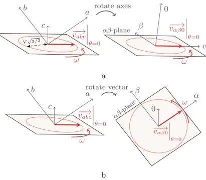
The power-invariant Clarke transformation is a pure rotation, such that the locus of a balanced three-phase quantity lies in the 𝑎𝑏-plane (this 𝑎𝑏-plane is referred to as

(38)

αβ-plane Vp3/2 a b c α β 0 ω _ω −−→ vabc θ=0 −−→ vαβ0 θ=0 rotate axes a αβ-plane a b c α β 0 −−→ vabc θ=0 −−→ vαβ0 θ=0 ω ω rotate vector b

Figure 3-1: The power invariant Clarke transformation: (a) Axes transformation perspective: rotate the 𝑎𝑏𝑐-axes such that the 𝑎-axis lines up with the vector 𝑣𝑎𝑏𝑐 at 𝜃 = 0, and the 𝑏-axis also lies in the rotated 𝑎𝑏-plane (𝛼𝛽-plane). The rotated 𝑎𝑏-axes become the 𝛼𝛽-axes respectively. The rotated 𝑐-axis becomes the 0-axis. (b) Vector transformation perspective: rotate the voltage vector 𝑣𝑎𝑏𝑐 such that its locus lies in the 𝑎𝑏-plane.

the 𝛼𝛽-plane after the transformation is performed). Fig. 3-1 illustrates the locus diagrams for the geometric power-invariant Clarke transformation.

All transformations can be visualised as either a coordinate (axes) transformation or as a vector transformation. Fig. 3-1a is the axes transformation where the vector is fixed and the 𝑎𝑏𝑐 axes are rotated such that the locus of a balanced system lies in the rotated𝑎𝑏-plane (ie the 𝛼𝛽-plane). Fig. 3-1b is the vector transformation, where the axes are fixed and the vector rotates such that its locus lies in the 𝑎𝑏-plane.

Note that there are infinite transformations that can achieve a locus that lies in the 𝑎𝑏-plane, but only one of these anchor the 𝛼-axis so that it is in line with the balanced Cartesian voltage when the phase angle is zero (𝜃 = 𝜔𝑡 + 𝜑 = 0), as seen in Fig. 3-1 . It will be shown later that this family of infinite transformations is given by Park’s matrix where substituting a value of theta anchors the𝛼-axis at a different location in the plane.

(39)

𝛼-axis appropriately one can determine the matrix associated with the power-invariant Clarke transformation. Eq. (2.5) (derived in Section 2.4) describes steps to find a matrix (e.g. 𝐴𝑐) that represents a linear transformation (𝑇𝑐). These steps require one to know how each orthonormal basis vector of a given space is affected by a transformation.

The inverse Clarke transformation𝑇_𝑐−1 is more convenient to derive geometrically than𝑇𝑐. One can visualise how𝑇−1

𝑐 transforms vectors by reading Fig. 3-1 from right to left. The inverse transformation rotates the unit vectors^e𝛼 and^e𝛽 such that they lie in the plane of −→𝑣𝑎𝑏𝑐. Thus, these transformed unit vectors 𝑇−1

𝑐 (ê𝛼), 𝑇𝑐−1(ê𝛽) have a direction given by −→𝑣𝑎𝑏𝑐 at angles of 𝜃 = 0 and 𝜃 = 𝜋/2 respectively. Whereas 𝑇𝑐 rotates the 𝑎𝑏𝑐 unit vectors ê𝑎, ê𝑏, ê𝑐 to a location that is inconvenient to determine.

−→

𝑣𝑎𝑏𝑐 = 𝑇_𝑐−1(−−→𝑣𝛼𝛽0) = 𝐴−1_𝑐 −−→𝑣𝛼𝛽0 (3.1)

The matrix 𝐴−1

𝑐 in Eq. (3.1) can be rewritten using Eq. (2.5):

𝐴−1_𝑐 = ⎡ ⎢ ⎢ ⎢ ⎢ ⎣ 𝑇 −1 𝑐 (ê𝛼) 𝑇𝑐−1(ê𝛽) 𝑇𝑐−1(ê0) ⎤ ⎥ ⎥ ⎥ ⎥ ⎦ (3.2)

These three steps of Eq. (3.2) are shown graphically in Fig. 3-2. Each step involves a rotation of a unit vector. The inverse power-invariant Clarke transformation 𝑇_𝑐−1 is applied to each of the three 𝛼𝛽0 unit vectors _{ê𝛼, ê𝛽, ê0_{}. Fig. 3-2a shows how ê}𝛼 is transformed under the inverse power-invariant Clarke transformation. Its transformed direction is given by the Cartesian voltage when the angle is zero:

𝑇_𝑐−1(^e𝛼) = −→ 𝑣𝑎𝑏𝑐⃒⃒_⃒

𝜃=0

‖−→𝑣_{𝑎𝑏𝑐‖} (3.3)

(40)

α β 0 −−→ vabc _θ=0 ˆ eα T−1 c (êα) a α β 0 −−→ vabc θ=π 2 ˆ eβ T−1 c (êβ) b α β _T₋₁ c (ê0) 0 ê0 c

Figure 3-2: Geometric power-invariant inverse Clarke derivation: (a) rotate ê𝛼 to align with the vector 𝑣𝑎𝑏𝑐 at 𝜃 = 0 (b) rotate ê𝛽 to align with the vector 𝑣𝑎𝑏𝑐 at 𝜃 = 𝜋/2 (c) rotate ê0 perpendicular to the plane. Note: This figure uses the vector transformation perspective shown in Fig. 3-1b. This perspective highlights how the unit vectors rotate, which allows us to evaluate Eq. (3.2)

with a radius given by Eq. (2.13). Substituting Eq. (2.13) into Eq. (3.3) gives:

𝑇_𝑐−1(^e𝛼) = 1 𝑉 √︂ 2 3−→𝑣𝑎𝑏𝑐 ⃒ ⃒ ⃒ ⃒ 𝜃=0 = √︂ 2 3 ⎡ ⎢ ⎢ ⎢ ⎢ ⎣ cos 𝜃 cos(︀𝜃₋ 2𝜋₃ )︀ cos(︀𝜃 + 2𝜋₃ )︀ ⎤ ⎥ ⎥ ⎥ ⎥ ⎦ ⃒ ⃒ ⃒ ⃒ 𝜃=0 (3.4) −→

𝑣𝑎𝑏𝑐 is evaluated when the angle is zero:

𝑇_𝑐−1(^e𝛼) = √︂ 2 3 [︂ 1 ₋1 2 − 1 2 ]︂| (3.5)

Fig. 3-2b illustrates how the the unit vector ^e𝛽 is rotated to align with the Cartesian voltage when the angle is 𝜋/2.

𝑇_𝑐−1(^e𝛽) = −→ 𝑣𝑎𝑏𝑐⃒⃒_⃒

𝜃=𝜋₂ ‖−→𝑣𝑎𝑏𝑐_‖

(41)

𝑇_𝑐−1(^e𝛽) = 1 𝑉 √︂ 2 3 −→𝑣𝑎𝑏𝑐 ⃒ ⃒ ⃒ ⃒ 𝜃=𝜋 2 = √︂ 2 3 [︂ 0 √₂3 ₋√₂3 ]︂| (3.6)

In Fig. 3-2c it was seen howê0 is rotated such that it is perpendicular to the plane of a balanced locus. Mathematically, this can be thought of as pointing in the direction of the cross product of ê𝛼 and ê𝛽, as given by the right-hand rule:

𝑇_𝑐−1(^e0) = −→ 𝑣𝑎𝑏𝑐⃒⃒_⃒ 𝜃=0× −→𝑣𝑎𝑏𝑐 ⃒ ⃒ ⃒ 𝜃=𝜋₂ ‖−→𝑣𝑎𝑏𝑐⃒⃒_⃒ 𝜃=0× −→𝑣𝑎𝑏𝑐 ⃒ ⃒ ⃒ 𝜃=𝜋 2 ‖ 𝑇_𝑐−1(^e0) = √︂ 2 3 [︂ 1 √ 2 1 √ 2 1 √ 2 ]︂| (3.7)

The three steps given by Eq. (3.5), Eq. (3.6) and Eq. (3.7) are combined with Eq. (3.2) to find𝐴−1 𝑐 . 𝐴−1 𝑐 = √︂ 2 3 ⎡ ⎢ ⎢ ⎢ ⎢ ⎣ 1 0 _√1 2 −1 2 √ 3 2 1 √ 2 −1 2 − √ 3 2 1 √ 2 ⎤ ⎥ ⎥ ⎥ ⎥ ⎦ (3.8) The matrix 𝐴−1

𝑐 is an orthogonal matrix because it is associated with a pure

rotation. This means its transpose is equal to its inverse, 𝐴𝑐=(︀𝐴−1 𝑐

)︀| .

3.1.2 Standard Clarke Transformation Derivation

The standard (amplitude-invariant) Clarke transformation was originally derived by Clarke in a manner shown in Fig. 2-3. This section geometrically derives the amplitude-invariant Clarke transformation which has become the standard version.

The standard Clarke transformation is a rotation and scaling, such that the locus of a balanced three-phase quantity lies in the𝑎𝑏-plane with a radius equal to the phase magnitude. It can be thought of as first applying the pure rotation described by the power-invariant Clarke transformation followed by a scaling operation. Eq. (2.13)

(42)

αβ-plane Vp3/2 V a b c α β 0 ω _ω −−→ v_abc θ=0 −−→ vαβ0 θ=0

rotate and rescale axes

a αβ-plane Vp3/2 _V a b c α β 0 −−→ v_abc θ=0 _−−→ vαβ0 θ=0 ω ω

rotate and scale vector

b

Figure 3-3: The standard (amplitude-invariant) Clarke transformation:(a) Axes trans-formation perspective: rotate the𝑎𝑏𝑐-axes such that the 𝑎-axis lines up with the vector 𝑣𝑎𝑏𝑐 at 𝜃 = 0, and the 𝑏-axis also lies in the plane. Stretch the rotated 𝑎𝑏-axes by √︀

3/2 such that the circle traced by 𝑣𝛼𝛽0 has a radius of 𝑉 , when referenced to the 𝛼𝛽-axes. The rotated and stretched 𝑎𝑏-axes become the 𝛼𝛽-axes respectively. The rotated 𝑐-axis becomes the 0-axis, and is stretched by√3 in order to agree with the definition of zero-sequence. (b) Vector transformation perspective: rotate the vector 𝑣𝑎𝑏𝑐 such that it lies in the𝑎𝑏-plane. Scale the rotated 𝑣𝑎𝑏𝑐 by √︀2/3 such that it has a length of 𝑉 when referenced to the 𝛼𝛽-plane. The 0-component of the vector 𝑣𝛼𝛽0 is scaled by 1/√3 in order to agree with the definition of zero-sequence.

shows that the locus of a balanced three-phase voltage is a circle of radius 𝑉√︀3/2. The standard Clarke transformation scales this locus, such that the circle has a radius of 𝑉 .

Fig. 3-3 illustrates the locus diagrams for the geometric amplitude-invariant Clarke transformation. Fig. 3-3a is the axes transformation where the vector is fixed and the 𝑎𝑏𝑐 axes are rotated such that the locus of a balanced system lies in the 𝛼𝛽-plane. The 𝛼 and 𝛽 axes are stretched by √︀3/2 such that the locus traced by a balanced voltage has a radius equal to𝑉 , the peak magnitude of the phase voltage. The 0-axis is stretched by √3 making this equivalent to the symmetrical components definition of zero-sequence. Whatever voltage exists on the 0-axis will appear with the same magnitude on the𝑎, 𝑏 and 𝑐 axes.

(43)

Fig. 3-3b is the vector transformation, where the axes are fixed and the vector rotates such that its locus lies in the 𝑎𝑏-plane. The vector’s 𝛼 and 𝛽 components are scaled by √︀2/3, meaning the locus of a balanced Cartesian vector will appear as a circle with a radius of 𝑉 when referenced to the 𝛼𝛽0 axes. The 0-axis is scaled by 1/√3 to match the symmetrical components definition of zero-sequence.

Just as with the power-invariant transformation, there are infinite transformations that can achieve a locus that lies in the𝑎𝑏-plane with the scaling described as above. However, only one of these ensure that the𝛼-axis is in line with the balanced Cartesian voltage when the phase angle is zero (𝜃 = 𝜔𝑡 + 𝜑 = 0).

The same procedure is followed as the power-invariant derivation. Once again, the

matrix 𝐴−1

𝑐 associated with the inverse transformation 𝑇𝑐−1 is found using Eq. (3.2). Please refer to Section 3.1.1 for a discussion on why the inverse Clarke transformation is derived.

The three steps described by Eq. (3.2) are shown graphically in Fig. 3-4. They involve transforming each of the three unit vectors under 𝑇_𝑐−1. Fig. 3-4a shows how ^

e𝛼 is transformed under the inverse standard Clarke transformation. ^e𝛼 is rotated and stretched by√︀3/2, making it equivalent to the per-unit Cartesian voltage when the angle is zero.

𝑇_𝑐−1(^e𝛼) = −→𝑣𝑎𝑏𝑐⃒⃒_⃒_{𝑉 =1} 𝜃=0 = ⎡ ⎢ ⎢ ⎢ ⎢ ⎣ 𝑉 cos 𝜃 𝑉 cos(︀𝜃− 2𝜋 3 )︀ 𝑉 cos(︀𝜃 + 2𝜋₃ )︀ ⎤ ⎥ ⎥ ⎥ ⎥ ⎦ ⃒ ⃒ ⃒_{𝑉 =1} 𝜃=0 𝑇_𝑐−1(^e𝛼) = [︂ 1 ₋1 2 − 1 2 ]︂| (3.9)

Similarly, Fig. 3-4b shows that^e𝛽 is rotated and stretched by √︀

3/2, making it equiv-alent to the per-unit Cartesian voltage when the angle is 𝜋/2.

𝑇_𝑐−1(^e𝛽) = −→𝑣𝑎𝑏𝑐 ⃒ ⃒ ⃒𝑉 =1 𝜃=𝜋 2 = [︂ 0 √3 2 − √ 3 2 ]︂| (3.10)

(44)

Fig. 3-4c explains how ^e0 is transformed. It points perpendicular to the plane in which the locus of −→𝑣𝑎𝑏𝑐 lies, and is scaled by√3. The scaling is necessary so that the 0-component agrees with the 0-sequence as defined by symmetrical components.

𝑇_𝑐−1(^e0) =√3 −→ 𝑣𝑎𝑏𝑐⃒⃒_⃒ 𝜃=0× −→𝑣𝑎𝑏𝑐 ⃒ ⃒ ⃒ 𝜃=𝜋₂ ‖−→𝑣𝑎𝑏𝑐⃒⃒_⃒ 𝜃=0× −→𝑣𝑎𝑏𝑐 ⃒ ⃒ ⃒ 𝜃=𝜋₂‖ = ⎡ ⎢ ⎢ ⎢ ⎢ ⎣ 1 1 1 ⎤ ⎥ ⎥ ⎥ ⎥ ⎦ (3.11)

The three transformed unit vectors given by Eq. (3.9), Eq. (3.10) and Eq. (3.11) are combined with Eq. (3.2) to find 𝐴−1

𝑐 . 𝐴−1_𝑐 = ⎡ ⎢ ⎢ ⎢ ⎢ ⎣ 1 0 1 −1 2 √ 3 2 1 −1 2 − √ 3 2 1 ⎤ ⎥ ⎥ ⎥ ⎥ ⎦ (3.12)

One can find𝐴𝑐 by taking the inverse of the matrix 𝐴−1

𝑐 .

3.2 Geometric Derivation of the Park

Transforma-tion

There are two versions of the Park transformation: the standard (amplitude-invariant) transformation and the power-invariant transformation. The derivation introduced by Park in Fig. 2-5 is the amplitude-invariant form, which is the most commonly used version. It is convenient because the magnitude of 𝑣𝑑 is the same as the magnitude of 𝑣𝑎 if two conditions are met: the voltages are balanced and the reference signal is in phase with phase 𝑎.

Previous approaches to deriving the Park transformation either use: trigonomet-ric projection with coplanar 𝑎𝑏𝑐 axes [19] or modifying symmetrical components to obtain Clarke’s matrix [15] and applying a rotation matrix. This section derives the Park transformation matrix using the geometric approach. The relationship between

(45)

α β 0 −−→ vabc V =1 θ=0 ˆ eα = T−1 c (êα) p 3/2 a α β 0 −−→ vabc V =1 θ=π 2 êβ Tc−1(êβ) = p 3/2 b α β Tc−1(ê0) =  11 1   0 ê0 c

Figure 3-4: Geometric standard (amplitude-invariant) inverse Clarke derivation:

(a) rotate ê𝛼 to align with the vector 𝑣𝑎𝑏𝑐 at 𝜃 = 0 and stretch by √︀3/2 (b) ro-tate ê𝛽 to align with the vector 𝑣𝑎𝑏𝑐 at 𝜃 = 𝜋₂ and stretch by √︀3/2 (c) rotate ê0 perpendicular to the plane and stretch by √3. Note: This figure uses the vector transformation perspective shown in Fig. 3-3b. This perspective highlights how the unit vectors stretch and rotate, which allows us to evaluate Eq. (3.2)

α β 0 α β d q 0 −−→ vαβ0 −−→vdq0 θ0 (θ0− θref) ω ω_ref ω

rotate axes CCW by θref

a α β 0 d q 0 −−→ v_dq0 θ0 (θ0− θref) −−→ vαβ0 ω (ω_{− ω}ref)

rotate vector CW by θref

b

Figure 3-5: The 𝛼𝛽0 to 𝑑𝑞0 transformation: (a) Axes transformation perspective:

rotate axes CCW about0-axis by 𝜃𝑟𝑒𝑓. (b) Vector transformation perspective: rotate vector CW about0-axis by 𝜃𝑟𝑒𝑓.

(46)

the Park and Clarke transformations as shown in Fig. 2-1 is utilised. The Park transformation can be decomposed into two consecutive transformations: the Clarke transformation followed by the 𝛼𝛽0 to 𝑑𝑞0 transformation. Section 3.1 details the geometric derivation of the Clarke transformation. This section completes the Park transformation matrix derivation by first deriving the 𝛼𝛽0 to 𝑑𝑞0 transformation. Then the Park transformation matrix is obtained by simple matrix multiplication. The overall geometric interpretation of the Park transformation is summarised in Fig. 2-6.

3.2.1 Transformation between Reference-Frames:

𝛼𝛽0 to 𝑑𝑞0

Transformation Derivation

The “transformation between reference-frames” or simply “frame-to-frame transfor-mation” in [2] is used in multimachine [4] and multi-inverter modelling [5]. Each device is modelled in its own 𝑑𝑞0 reference-frame, and each 𝑑𝑞0 frame may have a different angle𝜃 with respect to a common reference-frame. All devices can be trans-lated to the common reference-frame using the transformation between two rotating 𝑑𝑞0 frames [5]. The matrix describing this transformation has the same form as one that transforms from a stationary to a rotating 𝑑𝑞0 reference-frame. The trans-formation between two rotating 𝑑𝑞0 frames is equivalent to this thesis’ 𝛼𝛽0 to 𝑑𝑞0 transformation. Eq. (2.5) is used to derive this transformation, whereas the “transfor-mation between reference-frames” is derived in an alternative manner, using matrix multiplication: see section 3.10 of [2].

The 𝛼𝛽0 to 𝑑𝑞0 transformation can be geometrically interpreted in R3 _{as a pure} rotation about the 0-axis by a specified angle 𝜃𝑟𝑒𝑓. Fig. 3-5 illustrates the axes and vector transformation locus diagrams for the 𝛼𝛽0 to 𝑑𝑞0 transformation.

Fig. 3-5a is the axes transformation where the 𝛼𝛽0 axes are rotated counterclock-wise (CCW) about the0-axis by an angle 𝜃𝑟𝑒𝑓. It is helpful to visualise the motion of the axes and vectors to understand the𝛼𝛽0 to 𝑑𝑞0 transformation. Balanced systems have a Cartesian vector −−→𝑣𝛼𝛽0 that lies in the 𝛼𝛽-plane and rotates CCW about the

(47)

0-axis at speed 𝜔. Note that −−→𝑣𝛼𝛽0 has an arbitrary angle𝜃0 with respect to the𝛼-axis (𝜃0 = 𝜔𝑡 + 𝜑0). The𝛼𝛽0 axes are stationary and 𝜃0 increases with time.

The 𝑑𝑞0 axes of Fig. 3-5a are not stationary, unlike the 𝛼𝛽0 axes. These 𝑑𝑞0 axes rotate CCW about the 0-axis at an angle 𝜃𝑟𝑒𝑓 = 𝜔𝑟𝑒𝑓 𝑡 + 𝜑𝑟𝑒𝑓. −𝑣𝑑𝑞0−→ is the Cartesian vector referenced to 𝑑𝑞0 coordinates. If 𝜔𝑟𝑒𝑓 = 𝜔 then −−→𝑣𝑑𝑞0 will have 𝑣𝑑 and 𝑣𝑞 components which appear constant as the 𝑑𝑞0 axes are rotating at the same speed as the Cartesian vector −𝑣𝑑𝑞0−→. This case is illustrated by condition (i) of Fig. 2-2.

Fig. 3-5b is the vector transformation, where the axes are fixed and the Cartesian vector −−→𝑣𝛼𝛽0 is rotated clockwise (CW) about the 0-axis by an angle 𝜃𝑟𝑒𝑓. Thus, the vector has a net CCW angle of𝜃0_{− 𝜃}𝑟𝑒𝑓 relative to the 𝑑-axis. −−→𝑣𝛼𝛽0 is rotating CCW at an angular velocity 𝜔 when referenced to the 𝛼𝛽0 axes. When referenced to the 𝑑𝑞0 axes, the vector −−→𝑣𝑑𝑞0 has a CCW angular velocity of 𝜔− 𝜔𝑟𝑒𝑓. If 𝜔𝑟𝑒𝑓 = 𝜔 then −−→

𝑣𝑑𝑞0 will appear stationary on the 𝑑𝑞0 axes. −−→

𝑣𝑑𝑞0= 𝑇𝑑𝑞0(−−→𝑣𝛼𝛽0) = 𝐴𝑑𝑞0−−→𝑣𝛼𝛽0 (3.13)

The matrix 𝐴𝑑𝑞0 in Eq. (3.13) is found using Eq. (2.5). 𝑇𝑑𝑞0 is applied to each basis vector_{ê𝛼, ê𝛽, ê0_{} as shown in Fig. 3-6. 𝑇}𝑑𝑞0 rotates the vectorsê𝛼 andê𝛽 CW about the 0-axis by 𝜃𝑟𝑒𝑓. The components of 𝑇𝑑𝑞0(ê𝛼) and 𝑇𝑑𝑞0(ê𝛽) can be found using trigonometric relations.

𝑇𝑑𝑞0(^e𝛼) = [︁cos 𝜃 − sin 𝜃 0 ]︁|

(3.14)

𝑇𝑑𝑞0(^e𝛽) = [︁sin 𝜃 cos 𝜃 0 ]︁|

(3.15)

Fig. 3-6 shows how ^e0 is preserved under𝑇𝑑𝑞0.

𝑇𝑑𝑞0(^e0) = [︂

0 0 1 ]︂|

(3.16)

The three transformed unit vectors given by Eq. (3.14), Eq. (3.15) and Eq. (3.16) are combined with Eq. (2.5) to find𝐴𝑑𝑞0. The inverse transformation is found readily

(48)

αβ-plane α β 0 θ θ ˆ eα Tdq0(êα) êβ ê0 = Tdq0(ê0)

Figure 3-6: Geometric 𝛼𝛽0 to 𝑑𝑞0 derivation : (i) rotate ê𝛼 CW about 0-axis by 𝜃𝑟𝑒𝑓 (ii) rotate ê𝛽 CW about 0-axis by 𝜃𝑟𝑒𝑓 (iii) preserve ê0 under 𝑇𝑑𝑞0. Note: This figure uses the vector transformation perspective shown in Fig. 3-5b. This perspective highlights that the unit vectors rotate CW. While the axis transformation perspective in Fig. 3-5a has a CCW rotation of axes.

as the matrix is orthogonal (𝐴𝑑𝑞0|= 𝐴−1_𝑑𝑞0).

𝐴𝑑𝑞0 = ⎡ ⎢ ⎢ ⎢ ⎣ cos 𝜃 sin 𝜃 0 − sin 𝜃 cos 𝜃 0 0 0 1 ⎤ ⎥ ⎥ ⎥ ⎦ (3.17)

3.2.2 Power-Invariant Park Transformation Derivation

Park’s transformation is derived utilising the relationships between the transforma-tions in Fig. 2-1. The Park transformation is decomposed into the Clarke and 𝛼𝛽0 to𝑑𝑞0 transformations in Eq. (3.18).

−−→

𝑣𝑑𝑞0 = 𝑇𝑑𝑞0(𝑇𝑐(−→𝑣𝑎𝑏𝑐)) = 𝐴𝑑𝑞0𝐴𝑐−→𝑣𝑎𝑏𝑐= 𝐴𝑝−→𝑣𝑎𝑏𝑐 (3.18)

The power-invariant Park transformation is constructed using the power-invariant Clarke transformation of Eq. (3.8) and the 𝛼𝛽0 to 𝑑𝑞0 transformation in Eq. (3.17). Please refer to Section 3.1.1 for a comprehensive derivation of the power-invariant Clarke transformation. 𝐴𝑝 = 𝐴𝑑𝑞0𝐴𝑐= 𝐴𝑑𝑞0 √︂ 2 3 ⎡ ⎢ ⎢ ⎢ ⎢ ⎣ 1 −1 2 − 1 2 0 √₂3 −√3 2 1 √ 2 1 √ 2 1 √ 2 ⎤ ⎥ ⎥ ⎥ ⎥ ⎦

(49)

𝐴𝑝= √︂ 2 3 ⎡ ⎢ ⎢ ⎢ ⎢ ⎣ cos 𝜃 cos(︀𝜃₋2𝜋 3 )︀ cos(︀𝜃 + 2𝜋 3 )︀ − sin 𝜃 − sin(︀𝜃₋ 2𝜋 3 )︀ − sin(︀𝜃 + 2𝜋 3 )︀ 1 √ 2 1 √ 2 1 √ 2 ⎤ ⎥ ⎥ ⎥ ⎥ ⎦ (3.19)

3.2.3 Standard Park Transformation Derivation

The standard Park transformation can be determined in the same way as the power-invariant transformation using the relationships between the transformations (see Fig. 2-1) and Eq. (3.18). The difference is that the standard Clarke transformation of Eq. (3.12) is substituted for 𝐴𝑐. 𝐴𝑑𝑞0 is given by Eq. (3.17). Please refer to Section 3.1.2 for a comprehensive derivation of the standard Clarke transformation.

𝐴𝑝 = 𝐴𝑑𝑞0𝐴𝑐= 𝐴𝑑𝑞02 3 ⎡ ⎢ ⎢ ⎢ ⎢ ⎣ 1 −1 2 − 1 2 0 √₂3 −√3 2 1 2 1 2 1 2 ⎤ ⎥ ⎥ ⎥ ⎥ ⎦ 𝐴𝑝 = 2 3 ⎡ ⎢ ⎢ ⎢ ⎢ ⎣ cos 𝜃 cos(︀𝜃₋2𝜋 3 )︀ cos(︀𝜃 + 2𝜋 3 )︀ − sin 𝜃 − sin(︀𝜃₋ 2𝜋 3 )︀ − sin(︀𝜃 + 2𝜋 3 )︀ 1 2 1 2 1 2 ⎤ ⎥ ⎥ ⎥ ⎥ ⎦ (3.20)

3.2.4 Standard Park Transformation Derivation: A Direct

Ge-ometric Approach

Previously in this thesis, the Park transformation was decoupled into two operations, as shown in Fig. 2-6. Understanding the Park transformation as two consecutive operations highlights the geometric relationship between the Clarke, Park and frame-to-frame transformations.

(50)

transfor-d q 0 −−→ vabc −−→_v dq0 θ _θ ω ωref _ω

rotate and rescale axes

a b c Vp3/2 V a dq-plane Vp3/2 _V a b c d q 0 −−→ vabc −−→ vdq0 θ ω (ω_{− ω}ref)

rotate and scale vector

b

Figure 3-7: The standard (amplitude-invariant) Park transformation: (a) Axes trans-formation perspective: rotate the 𝑎𝑏𝑐-axes such that the 𝑎-axis lines up with the vector 𝑣𝑎𝑏𝑐 at 𝜃, and the 𝑏-axis also lies in the plane. Stretch the rotated 𝑎𝑏-axes by √︀3/2 such that 𝑣𝑑𝑞0 has a length of 𝑉 , when referenced to the 𝑑𝑞-axes. The rotated and stretched 𝑎𝑏-axes become the 𝑑𝑞-axes respectively. The rotated 𝑐-axis becomes the 0-axis, and is stretched by √3 in order to agree with the definition of zero-sequence. (b) Vector transformation perspective: rotate the vector 𝑣𝑎𝑏𝑐 such that it lies in the 𝑎𝑏-plane, and it rotates CCW about the 0-axis at a speed 𝜔_{− 𝜔𝑟𝑒𝑓}. Scale the rotated 𝑣𝑎𝑏𝑐 by √︀2/3 such that it has a length of 𝑉 when referenced to the 𝑑𝑞-plane. The 0-component of the vector 𝑣𝑑𝑞0 is scaled by 1/√3 in order to agree with the definition of zero-sequence. Note: In both figures (a) and (b) the voltages are balanced, meaning the locus of 𝑣𝑎𝑏𝑐 is a circle of radius 𝑉√︀3/2.

mation from 𝑎𝑏𝑐 to 𝑑𝑞0, without considering an intermediate 𝛼𝛽0 reference frame. In this section, this direct derivation is shown for the standard Park transformation us-ing the approach outlined in Section 2.4 and given by Eq. (2.5). The power-invariant Park transformation can also be found directly using a similar approach.

Fig. 3-7 illustrates the standard 𝑎𝑏𝑐 to 𝑑𝑞0 transformation. This is plotted for the case where the 𝑑-axis lines up with the vector −−→𝑣𝑑𝑞0. Refer to Fig. 3-5 for the case where the𝑑-axis may not be in line with −−→𝑣𝑑𝑞0. Fig. 3-7a shows the axis transformation, where the axes can be seen rotating and stretching so that −𝑣𝑑𝑞0−→ traces out a circle of

Decentralized power systems : reference-frame theory and stability region generation

Decentralized Power Systems: Reference-Frame

Theory and Stability Region Generation

by

Colm J. O’Rourke

B.E., Energy Systems Engineering

National University of Ireland, Galway (2013)

S.M., Electrical Engineering and Computer Science

Massachusetts Institute of Technology (2015)

Submitted to the Department of Electrical Engineering and Computer

Science

in partial fulfillment of the requirements for the degree of

Doctor of Philosophy in Electrical Engineering and Computer Science

at the

MASSACHUSETTS INSTITUTE OF TECHNOLOGY

May 2020

c

○ Massachusetts Institute of Technology 2020. All rights reserved.

Author . . . .

Department of Electrical Engineering and Computer Science

May 15, 2020

Certified by . . . .

James L. Kirtley

Professor of Electrical Engineering

Thesis Supervisor

Accepted by . . . .

Leslie A. Kolodziejski

Professor of Electrical Engineering and Computer Science

Chair, Department Committee on Graduate Students

Decentralized Power Systems: Reference-Frame Theory and

Stability Region Generation

by

Colm J. O’Rourke

Abstract

Acknowledgments

Contents

I

A Geometric Interpretation of Reference-Frames

17

II

Stability Region Generation using Machine Learning

57

List of Figures

List of Tables

Chapter 1

Introduction

1.1

Thesis Structure

Part I

A Geometric Interpretation of

Reference-Frames

Chapter 2

Reference-Frame Theory

2.1

Overview and Motivation

2.2

Previous Work

2.2.1

Review of the Clarke and Park Transformations

v

v

v

abc

2.2.2

Review of the Arbitrary Reference-Frame

2.3

Contributions to Reference-Frame Theory

2.4

Review of Linear Transformations

!v

!

v

!v

!v

!v

!

!

!

2.5

Cartesian Representation of Three-Phase