Évaluation de la biodiversité des invertébrés marins
dans les ports commerciaux de l'Arctique grâce à l'ADN
environnemental
Mémoire
Noémie Leduc
Maîtrise en biologie - avec mémoire
Maître ès sciences (M. Sc.)
Évaluation de la biodiversité des invertébrés
marins dans les ports commerciaux de l’Arctique
grâce à l’ADN environnemental
Mémoire
Noémie Leduc
Sous la direction de :
Louis Bernatchez, directeur de recherche
Philippe Archambault, codirecteur de recherche
Résumé
D’abord méconnue puis longuement sous-estimée, la biodiversité de l’Arctique fait maintenant face à d’importantes altérations sous les effets combinés des changements climatiques ainsi que l’augmentation des activités commerciales dans l’Arctique canadien. Ces altérations ne sont pas sans risque pour les communautés d’invertébrés marins, particulièrement dans les zones sensibles telles que les ports commerciaux. La protection de la biodiversité représente un enjeu majeur, nécessitant une bonne compréhension de l’organisation spatiale des espèces au moyen d’indices de biodiversité tels que les indices alpha, beta et gamma, de même que le développement de méthodes de détection efficace. Dans le cadre de ce projet de maîtrise, la biodiversité obtenue à l’aide de méthodes d’échantillonnage traditionnelle fut comparée à la biodiversité détectée par l’ADN environnementale (ADNe), grâce au metabarcoding des gènes COI et 18S, afin de documenter les patrons de biodiversité des communautés d’invertébrés marins à différentes échelles spatiales. À partir d’échantillons d’eau de 250 ml récoltés à trois différentes profondeurs au sein des ports de Churchill, Baie Déception et Iqaluit, il fut possible de déceler la présence de 202 genres répartis dans plus de 15 phyla. De ces organismes, seulement 9 à 15% furent également collectés par les méthodes traditionnelles, révélant ainsi l’existence de différences significatives au niveau de la richesse et de la composition des communautés entre ces différentes approches d’échantillonnage. Outre ces différences majeures, cette étude a permis de démontrer une réduction de la biodiversité beta dans les communautés détecter à l’aide de l’ADNe comparativement aux communautés identifiées par la collecte de spécimens. Cette homogénéisation de la biodiversité souligne le rôle non négligeable de la dispersion de l’ADNe ainsi que l’influence notoire des stades de vie pélagique dans sa détection. Les résultats obtenus dans le cadre de cette étude mettent bien en évidence le potentiel du metabarcoding d’ADNe tout en insistant sur son caractère complémentaire face aux méthodes traditionnelles pour d’éventuelles applications en gestion et conservation des communautés d’invertébrés marins de l’Arctique.
Abstract
Arctic biodiversity has long been underestimated and is now facing rapid transformations due to ongoing climate change and other impacts including shipping activities. These changes are placing marine coastal invertebrate communities at greater risk, especially in sensitive areas such as commercial ports. Preserving biodiversity is a significant challenge, going far beyond the protection of charismatic species and involving suitable knowledge of the organization of species in space. Therefore, knowledge of alpha, beta and gamma biodiversity indices are of great importance in achieving this objective together with new cost-effective approaches to monitor changes in biodiversity. This study compares metabarcoding of COI mitochondrial genes and 18S rRNA genes from environmental DNA (eDNA) water samples with standard species collection methods to document patterns of invertebrate communities at various spatial scales. Water samples (250 mL) were collected at three different depths within three Canadian Arctic ports; Churchill, MB, Iqaluit, NU and Deception Bay, QC. From these samples, 202 genera distributed across more than 15 phyla were detected using eDNA metabarcoding, of which only 9% to 15% were also identified through species collection at the same sites. Significant differences in taxonomic richness and community composition were observed between eDNA and species collections, both on local and regional scales. This study shows that eDNA dispersion in the Arctic Ocean reduces beta diversity in comparison to species collection while emphasizing the importance of pelagic life stages for eDNA detection. This study highlights the potential of eDNA metabarcoding to assess large-scale arctic marine invertebrate diversity while emphasizing that eDNA and species collection should be considered as complementary tools for providing a more holistic picture of the marine invertebrate communities living in coastal areas.
Table des matières
Résumé ... ii
Abstract ... iii
Table des matières ... iv
Liste des tableaux ... vi
Liste des figures ... vii
Remerciements ... ix
Avant-propos ... xi
Introduction ... 1
Problématique générale ... 1
L’Arctique dans un monde en changement ... 2
La biodiversité comme unité de gestion pour la conservation ... 3
Indices de biodiversité ... 3
Méthodes pour recenser la biodiversité ... 5
L’utilisation d’outils moléculaires ... 5
Métabarcoding ... 5
ADN environnementale (ADNe) ... 6
Les invertébrés marins ... 8
Contexte du projet ... 9
Objectifs ... 10
Chapter I: Comparing eDNA metabarcoding and species collection for documenting Arctic metazoan biodiversity ... 11 Résumé ... 12 Abstract ... 13 Introduction ... 14 Methods ... 17 Sample collection ... 17 Species collection ... 18
Environmental DNA samples ... 19
Metabarcoding ... 20
Environmental DNA extraction, amplification and sequencing ... 20
Bioinformatics ... 21
Data analysis ... 22
Results ... 23
Sequencing quality ... 23
Arctic coastal gamma diversity ... 25
Alpha biodiversity ... 29
Beta diversity ... 32
Origin of coastal eDNA ... 33
Overall biodiversity and community structure ... 35
Transport and homogenization of eDNA... 38
Origins of eDNA ... 40
Role of eDNA in Arctic conservation ... 41
Acknowledgement ... 43
Annexe (Supporting information) ... 44
Conclusion ... 55
ADNe vs. collecte d’espèces ... 56
Origine, détection et transport de l’ADNe ... 57
Faiblesses et limites du métabarcoding d’ADN environnemental ... 58
Applications et perspectives futures pour la protection de la biodiversité ... 59
Liste des tableaux
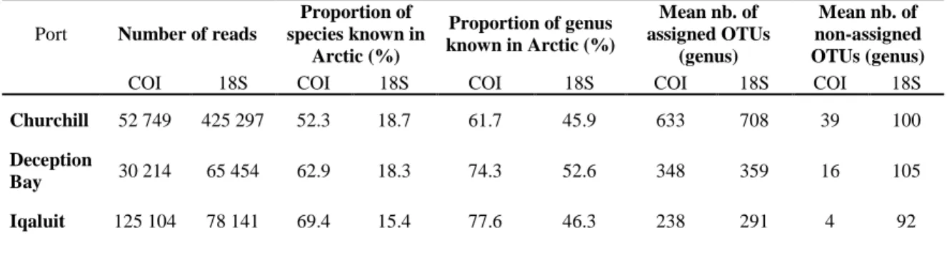
Table 1. Summary of the numbers of reads, the proportion of species and genera present in the Arctic historic database and the mean number of OTUs for the COI primers set and the 18S primers set assigned and non assigned on BOLD and SILVA for each port.
Table 2. Summary of richness, alpha and beta biodiversity indices for the eDNA and species collection of marine invertebrates communities on abundance data after Hellinger transformation (Shannon and Pielou indices) and presence/absence transformation (Beta index). COI primer sets and 18S primer sets are added together.
Table S1. Barque 1.5.1 specific commands for preparation and analysis of pair-end reads. The sequences from the different COI and 18S primers set were added together.
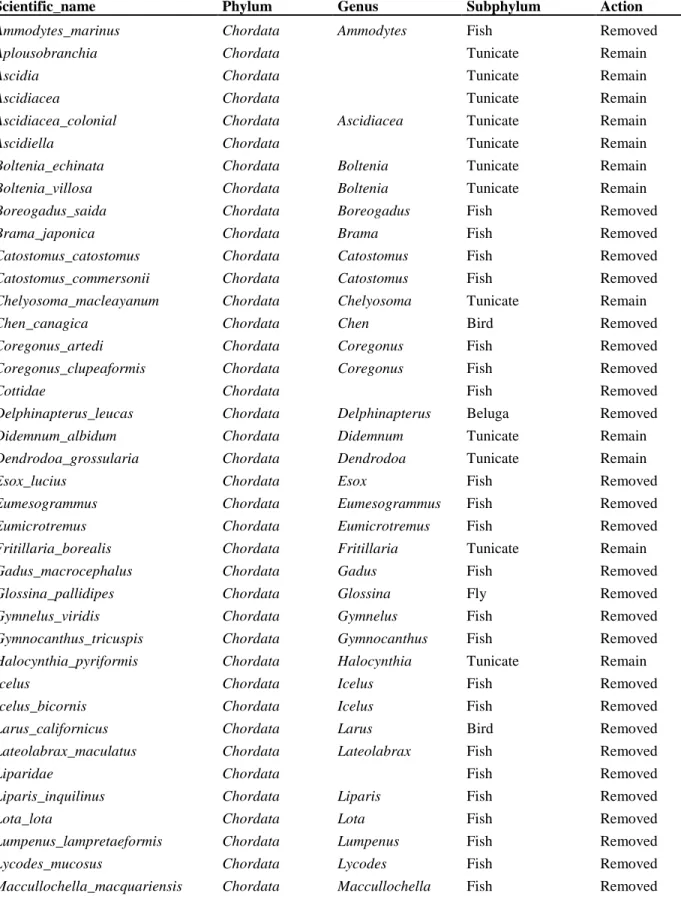
Table S2. Chordata taxa present in the eDNA data set (COI and 18S primers set added together) and the appropriate action taken.
Table S3. Genera found in the negative field controls and the appropriate action taken against the contamination according to COI and 18S primers set.
Table S4. Summary of PERMANOVA statistics tests on marine invertebrates communities for the phylum relative abundance (number of taxa), Pielou evenness index and alpha richness. The analyses were performed with method = "bray" for phylum relative abundance while it was performed with method = "euclidian" for Pielou evenness and alpha richness. Table S5. Summary of the correlation between dissimilarity and distance across the sites within Churchill, Deception Bay and Iqaluit ports based on incidence data for the different sampling methods.
Table S6. Summary of the main phyla identified by sampling collection sampling methods among Churchill, Deception Bay and Iqaluit ports and their respective presence in BOLD and SILVA public genetic databases.
Liste des figures
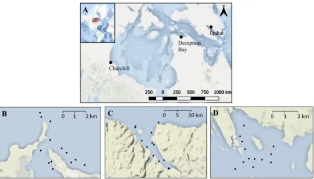
Figure 1. Geographical location of Churchill, Deception Bay and Iqaluit ports in the Canadian Arctic (map A) and distribution of stations within Churchill (map B), Deception Bay (map C) and Iqaluit (map D).
Figure 2. Individual-based rarefaction curves of eDNA, benthos and zooplankton genera for Churchill (blue), Deception Bay (yellow) and Iqaluit ports (magenta) based on incidence data.
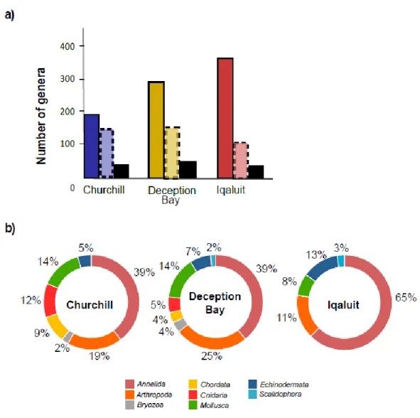
Figure 3. a) Barplots of the number of taxa found in Churchill (blue), Deception Bay (yellow) and Iqaluit (red). Darker bands represent species collection methods while paler bands with dashed outline represent eDNA and black bands represent the number of genera in common between eDNA and species collection. b) Phylum relative proportion of commun genera between eDNA and species collection based on incidence data. COI and 18S primer sets are added together for both a) and b).
Figure 4. Marine invertebrate taxonomic composition at the phylum level for eDNA and species collection methods, respectively, within Churchill, Deception Bay and Iqaluit ports, based on incidence data. The COI and 18S regions are added together for the eDNA barplot while the benthic trawl, core, grab and net tows samples are added together for the species collection barplot.
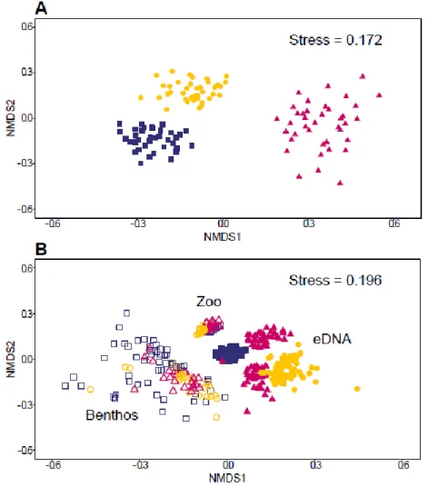
Figure 5. Biodiversity differences A) among ports based on eDNA only and B) among sampling methods within ports. Ordination of taxonomic composition (genera) calculated using Sorensen index (incidence based) with each data point representing a specific sample; blue squares represent Churchill, yellow dots represent Deception Bay and magenta triangles represent Iqaluit. Filled symbols are associated with eDNA while empty symbols are associated with species collections.
Figure 6. Boxplot on alpha diversity for the genera richness and Pielou evenness index in Churchill, Deception Bay and Iqaluit ports for eDNA (A, C) and species collection (B, D). These analyses were performed on abundance data with Hellinger transformation, COI and 18S primer sets are added together for the eDNA boxplot.
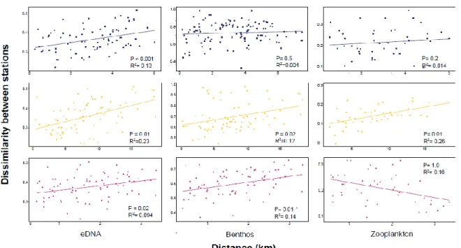
Figure 7. Sorensen dissimilarity index between pairs of stations as a function of distance between the stations based on incidence data (presence/absence transformation on abundance) for different sampling methods (eDNA and species collections of benthos and zooplankton) in Churchill (blue), Deception Bay (yellow) and Iqaluit (magenta).
net tows. The sum of the detection of each taxa (i.e. presence/absence) have been combined for all primer sets.
Figure S1. The number of Operational taxonomic units (OTUs) assigned and not assigned on NCBI to the genus level for the COI primers set (COI1 and COI2) and the 18S primers set (Tareuk and 18S). The assigned OTUs are represented by the grey section of the barplot while the not assigned OTUs are represented by the red section of the barplot. The pourcentage written in red represented the mean of the 4 primers for not assigned OTUs in each port.
Figure S2. Boxplot on alpha diversity for Shannon biodiversity index in Churchill, Deception Bay and Iqaluit ports. These analyses were performed on abundance data with Hellinger transformation, COI and 18S primer sets are added together for the eDNA boxplot.
Remerciements
Je voudrais avant tout remercier mon directeur de recherche, le Dr Louis Bernatchez, que ce soit des plongées en apnée dans les îles Galápagos, aux salles de cours puis finalement comme directeur de recherche, ta passion pour la science et la génétique est contagieuse et ne cessera de m’impressionner. Merci de m’avoir accueillie dans ton laboratoire de même que la grande famille qui le compose ainsi que pour ta confiance en moi depuis mes tout début dans le domaine de la biologie moléculaire. Ces trois dernières années furent extrêmement riches en expériences, tant sur le plan personnel que professionnel en grande partie grâce aux opportunités que tu m’as offertes dans le cadre de ma maîtrise.
J’aimerais également remercier mon codirecteur de recherche, le Dr Philippe Archambault, pour sa patience, son expertise incroyable ainsi que son émerveillement devant chacun de mes petits résultats. Merci Phil pour ton écoute et tes précieux conseils, qui ont su me remonter le moral dans les moments de doutes.
La réussite de ce projet repose également sur la participation de plusieurs personnes. Je tiens à remercier Anaïs Lacoursière-Roussel pour m’avoir guidée dès mes premiers pas en tant qu’étudiante à la maîtrise et pour avoir investi beaucoup de temps et d’énergie dans l’ensemble du projet, de son élaboration jusqu’à la collecte des précieux échantillons et finalement son aboutissement avec le mémoire ci-présent. Je voudrais également remercier Kimberly Howland, sans qui ce projet n’aurait pas pu voir le jour tel qu’il est aujourd’hui de même que Maelle Sevellec, qui malgré le décalage horaire a toujours été présente avec le sourire à nos rencontres Skype et a su m’encourager et me fournir de précieux conseils pour la conception de ce manuscript.
expertise en laboratoire de même que pour leurs nombreux conseils. Merci à notre bioinformaticien Éric Normandeau pour son souci du détail et sa disponibilité pour répondre aux nombreuses embuches qu’accompagne souvent la bioinformatique. Merci à Damien Boivin-Delisle, mon "eDNA partner", pour nos discussions diverses mais toujours enrichissantes de même que nos divagations par certains moments. Finalement merci à Valérie Cypihot du laboratoire Archambault, pour son amitié, son aide sur le terrain, sa compagnie lors de nos congrès ainsi que ses conseils.
Pour finir, un grand merci aux membres de ma famille et de ma belle-famille pour leur encouragement, et par-dessus tout mes parents pour leur soutien et leur confiance en moi depuis le début de mes études. Je remercie mes amies de la boite de céréales, plus spécialement Justine Létourneau pour son aide et sa compagnie de grande qualité au sein du laboratoire. Finalement je remercie tout spécialement mon copain, Gabriel, pour son support inconditionnel depuis le début de ma maîtrise, son sens de l’humour et son optimisme au quotidien.
Avant-propos
Ce mémoire est principalement composé d’un article intitulé « Comparing eDNA metabarcoding and species collection for documenting Arctic metazoan biodiversity ». Cet article a été soumis à la revue « Environmental DNA » et est actuellement en processus de révision.
Les co-auteurs sont mesdames Kimberly Howland, Maelle Sevellec, Anaïs Lacoursière-Roussel, monsieur Éric Normandeau, mon co-directeur Philippe Archambault et mon directeur Louis Bernatchez.
Anaïs Lacoursière-Roussel, Kimberly Howland, ont élaboré l’étude globale dans lequel s’inscrit mon projet de maîtrise, organisé les campagnes d’échantillonnage de même que participé à la collecte d’échantillons sur le terrain. Éric Normandeau a conçu le pipeline bioinformatique ayant servi aux traitements des données d’ADNe suite au séquençage. Maelle Sevellec a contribuer aux analyses statistiques de même qu’à la rédaction de l’article dans son ensemble. Pour ma part, j’ai réalisé le travail sur le terrain et au laboratoire, rédigé l’article (auteure principale) et effectué l’analyse et l’interprétation des résultats avec l’aide de mes co-auteurs. Tous les co-auteurs ont également collaboré à la révision du manuscript.
Ce projet a été financé par le réseau de centres d’excellence ArcticNet, le programme fédéral Savoir polaire Canada (POLAIRE) ainsi que le regroupement Québec-Océan.
Introduction
Problématique générale
Depuis le Sommet de la Terre à Rio de Janeiro en 1992, l’intérêt porté à la biodiversité de même qu’aux conséquences possibles que celle-ci peut engendrer en cas de perte, n’a cessé de croître et de stimuler la recherche scientifique (Cardinale et al. 2012). Malgré cet intérêt notoire pour la biodiversité, l’anthropocène plonge la planète dans une importante extinction de masse, où la surexploitation, la destruction des habitats et les changements climatiques entraînent chaque jour la disparition de plusieurs espèces (Young et al. 2016). Le maintien de la biodiversité est nécessaire afin de soutenir la stabilité des processus écosystémiques dans des environnement en perpétuels changement (Loreau et de Mazancourt 2013) de ce fait, son déclin actuel représente une crise majeure ainsi qu’un défi considérable pour le 21ème siècle (Vié et al. 2009).
Parmi les habitats les plus affectés par cette crise on retrouve l’océan Arctique (Jørgensen et al. 2016). Ce dernier étant le plus petit océan de la planète mais également le moins connu de tous en raison de son emplacement géographique, ses conditions météorologiques hostiles ainsi que sa couverture de glace récurrente (National Research Council 1995). Considéré jusqu’à récemment comme l’un des endroits les plus intact du globe (UNESCO 2010), l’océan Arctique possède une biodiversité bien supérieure à ce qui était estimé en raison de connaissances rudimentaires à son sujet (Darnis et al. 2012). Face aux nombreux enjeux existants, un besoin urgent est né afin de pallier au manque d’informations relatif à la diversité de même qu’à la distribution des espèces présente dans l’Arctique et ce dans l’espoir de pouvoir minimiser les impacts en grande partie imposés par l’humain sur la biodiversité marine de cet océan (Bluhm et al. 2011).
L’Arctique dans un monde en changement
Les changements climatiques actuels causent d’importantes altérations aux patrons de biodiversité à l’échelle de la planète par l’extinction de nombreuses espèces. Globalement, près de 8% des extinctions d’espèces dans le futur découleraient directement de ces changements climatiques (Urban 2015). Les habitats marins ne sont pas épargnés par cette crise, l’augmentation de la température de l’eau, l’acidification des océans, ainsi que les changements physicochimiques reliés à ces phénomènes causent la dégradation des habitats (Hoegh-Guldberg et Bruno 2010). De ces changements climatiques résulte également une importante fonte des glaces qui façonne de nouveaux paysages (Kintisch 2015) et entraine par le fait même une augmentation considérable des activités humaines dans certains secteurs maritimes (Ruffilli 2011) .
Lors de la saison estivale, alors que la couverture de glace est à son minimum, c’est 75% de son volume qui est perdu depuis 1979 (Kintisch 2015). Cette perte importante de glace dans l’océan Arctique permet l’ouverture de nouveaux chemins pour la navigation des bateaux commerciaux (Vermeij et Roopnarine 2008) en plus d’augmenter la durée où la navigation est praticable à certains endroits. Dans le cadre de sa Stratégie pour le Nord, le gouvernement du Canada compte promouvoir le développement social et économique des communautés nordiques, ce qui combiné à la popularité grandissante de l’Arctique pour le tourisme et l’industrie des croisières augmentera considérablement la circulation maritime au cours des prochaines décennies (Gavrilchuk et al. 2013).
Les effets associés du réchauffement climatique ainsi que de l’augmentation des activités anthropiques auront des répercussions directes sur la biodiversité ainsi que la distribution des communautés marines. Ces conséquences seront d’autant plus considérables pour les régions côtières, qui sont sujettes à de plus grandes pertes de diversité en raison des utilisations
qui transportent et déchargent une quantité non négligeable d’organismes à des distances qui dépassent largement leur capacité naturelle de dispersion (Casas-Monroy et al. 2014), une augmentation significative du risque d’introduction d’espèces exotiques est attendu dans l’Arctique canadien au cours des prochaines années (Mooney et Cleland 2001; Casas-Monroy et al. 2014). Dans certains cas, ces espèces exotiques peuvent devenir des espèces envahissantes, ayant la capacité d’engendrer de profonds changements écologiques (Carlton 1993) et causer des pertes majeures de biodiversité (Williamson 1999).
Dans un tel contexte, où la biodiversité de même que la composition des communautés marines sont appelés à connaître d’importantes altérations liées à divers facteurs, des méthodes permettant une détection rapide et efficiente des changements de biodiversité sont plus que nécessaires.
La biodiversité comme unité de gestion pour la conservation
Indices de biodiversité
La biodiversité, concept ayant vu le jour dans les années 1980 (Pimm 2001), décrit la variété structurelle et fonctionnelle de l’ensemble des formes de vie tant au niveau de la génétique, des populations que des écosystèmes (Sandlund et al. 1992). Depuis quelques années, la conservation de la biodiversité marine devient progressivement un objectif capital en gestion environnementale (Spalding et al. 2007), nécessitant ainsi suffisamment d’informations et de bases de données sur les organismes concernés (Laurila-Pant et al. 2015). Les indices de biodiversité constituent une approche écologique classique afin d’évaluer la biodiversité, ceux-ci prenant en considération deux aspects majeurs des communautés soit la richesse spécifique ainsi que l’abondance relative des individus au sein de chaque espèce (Hamilton 2005, Laurila-Pant et al. 2015). Plusieurs indices existent afin de pouvoir quantifier le rythme auquel la biodiversité varie dans le temps et l’espace (Gaston 2000), que ce soit au niveau de l’espèce ou de la communauté et selon différentes échelles spatiales et/ou organisationnelles à travers les valeurs descriptives alpha, beta et gamma.
La biodiversité alpha représente l’assemblage d’une communauté à basse échelle et constitue la plus petite mesure de la biodiversité (MacArthur 1965), elle reflète habituellement la richesse spécifique d’un lieu. C’est également l’indice de biodiversité le plus utilisé et revêt d’une importance cruciale pour la conservation (Socolar et al. 2015). Comme cet indice est fortement influencé par la taille des échantillons ainsi que par l’envergure des lieux échantillonnés et peut être biaisée par ces paramètres il est important d’utiliser des techniques statistiques qui tiennent comptent de ces derniers, telle que la standardisation des données (Roff et Mark 2011).
La diversité beta, aussi appelée « turnover diversity » fait référence au degré de changement dans la composition des espèces le long d’un certain gradient (Gray 2000). Cet indice peut être interprété comme le taux de variation dans la composition des espèces par rapport à l’environnement ou au sein de communautés (Roff et Mark 2011; Van Dyke 2010), en fonction de processus menant à l’homogénéisation ou l’hétérogénéisation des communautés. De ce fait, une bonne compréhension de la diversité beta est essentielle afin de protéger la biodiversité régionale ainsi que dans l’optique de contribuer directement aux plans de conservation (Socolar et al. 2015). La diversité beta est une mesure d’autant plus importante pour les communautés sujettes à d’importantes perturbations (Mori et al. 2018).
Finalement, la diversité gamma constitue quant à elle la diversité totale d’une région donnée, représentant ainsi la richesse spécifique de chacun des différents habitats au sein de celle-ci. Puisque l’indice de biodiversité gamma désigne le regroupement d’indice de biodiversité alpha pour une région, celle-ci est exprimé dans les mêmes unités que cette dernière (Laurila-Pant et al. 2015).
Méthodes pour recenser la biodiversité
Actuellement, et depuis plusieurs décennies, la majorité des suivis de biodiversité en milieu aquatique sont basés sur l’identification morphologique des organismes, que ce soit au moyen de sondages visuels ou du dénombrement des individus directement sur le terrain. Ces méthodes requièrent toutefois des notions de taxonomie avancées, dans un contexte où les spécialistes pratiquant cette discipline se font de plus en plus rares (Archambault et al., 2010), créant ainsi une demande pour des approches d’identifications alternatives (Radulovici et al. 2010 ; Thomsen et Willerslev 2015). De plus, certaines techniques d’inventaires traditionnelles comme le chalutage de fond peuvent se révéler invasives et dommageables pour les espèces et les écosystèmes (Baldwin et al. 1996; Jones 1992; Robertson et Smith-Vaniz 2008). À cela s’ajoute la logistique souvent complexe associée aux instruments d’échantillonnage traditionnel (chalut, benne Van Veen, filets) dans des régions éloignées et/ou difficiles d’accès tel que l’Arctique (Jorgensen et al. 2016). Le développement de nouveaux outils non-invasifs permettrait de remédier à certain de ces désavantages et améliorerait potentiellement la capacité d’échantillonner la biodiversité marine à large échelle tout en ayant un minimum d’impacts négatifs sur celle-ci.
L’utilisation d’outils moléculaires
Métabarcoding
L’identification simultanée de plusieurs taxons par code-barres ADN (métabarcoding) se veut être une méthode fort attrayante afin de décrire la composition de communautés biologiques complexes ainsi que pour en estimer la biodiversité (Brown et al. 2015). Cette technique est utilisée depuis plusieurs décennies chez les microbiologistes (Coissac et al. 2012) et exploite la diversité génétique présente au sein de séquences particulières d’ADN chez les organismes afin de les distinguer les uns des autres et de les identifier. Ces séquences représentent des identifiants génétiques se trouvant à l’intérieur de chaque cellule (Hebert et al. 2003). Ces marqueurs génétiques doivent être le plus universel possible tout en ayant juste assez de dissimilitudes pour pouvoir différencier les espèces ou les groupes d’intérêt ainsi, le
choix des marqueurs d’ADN appropriés dépend fortement de la résolution désirée pour l’identification (Drummond et al., 2015).
Le gène de la sous-unité I du cytochrome c (COI), un gène codant une protéine de l’ADN mitochondrial (ADNmt), est souvent défini comme le marqueur de référence pour le métabarcoding des métazoaires, car celui-ci permet d’identifier un nombre abondant de phylum en plus d’avoir une variation génétique permettant d’effectuer le discernement au niveau des espèces (Hebert et al. 2003; Deagle et al., 2014). De plus, l’ADNmt est davantage présent que l’ADN nucléaire au sein des cellules, et ce même dans des milieux qui contiennent de faibles concentrations d’ADN et lorsque celui-ci est dégradé (Rees et al. 2014). Le marqueur 18S, gène présent sur l’ARN ribosomique (ARNr) est aussi largement utilisé en raison de sa taille et de son abondance dans le génome, en plus de sa caractéristique à être peu sujet aux mutations, ce qui fait de lui un bon candidat pour distinguer les différents phyla entre eux (Carugati et al. 2015). Les marqueurs COI et 18S sont souvent ciblés comme code-barres génétiques en raison de leur accessibilité dans les bases de données publiques telles que BOLD, SILVA et GenBank.
ADN environnementale (ADNe)
Depuis que Ficetola et al. (2008) ont démontré qu’il était possible de détecter la présence de vertébrés en utilisant l’ADNe contenu dans des échantillons d’eau, l’intérêt pour l’ADNe comme outil pour la conservation des poissons, des invertébrés aquatiques et des amphibiens s’est rapidement intensifié (Goldberg et al. 2015). Comme toutes espèces interagissant avec leur environnement, celles-ci rejettent constamment de leur ADN dans les endroits qu’elles fréquentent (Thomsen et Willerslev 2015). Cet ADN représente du matériel génétique pouvant provenir de gamètes, d’œufs, de fèces, d’urine, de mucus, de salive, ou encore de sang (Bohmann et al. 2014; Keskin 2014; Rees et al. 2014). Une fois relâché dans
de santé, le sexe et la densité de ceux-ci, sans oublier la température du milieu puisque cette dernière possède une influence majeure sur le métabolisme des organismes (Goldberg et al. 2015; Klymus et al. 2015; Lacoursière-Roussel et al. 2016). La préservation de l’ADN varie grandement selon le milieu allant de quelques semaines dans les eaux tempérées à plusieurs milliers d’années dans le permafrost, tout dépendamment de certains facteurs. Les endonucléases présentes dans le milieu, l’eau, les radiations UV ainsi que l’action des bactéries ou champignons représentent tous des conditions environnementales qui contribuent à la dégradation de l’ADN dans différents écosystèmes (Shapiro 2008).
L’utilisation de l’ADNe constitue non seulement une méthode surpassant certains défis techniques, mais représente également une méthode non invasive qui contribue à diminuer grandement les perturbations dans les habitats des espèces recensées (Bohmann et al. 2014). L’utilisation de l’ADNe s’est également révélée être plus efficiente pour détecter les espèces rares ainsi que les espèces difficiles d’approche comparativement aux méthodes d’échantillonnage traditionnelle (Goldberg et al. 2015; Smart et al. 2015). Combiné au metabarcoding, l’ADNe peut fournir un portrait instantané des communautés locales sans avoir à échantillonner directement chaque organisme présent. Ces nouveaux outils moléculaires représentent une nouvelle méthode de caractérisation de la biodiversité remplie de potentiel, constituant une opportunité d’augmenter considérablement l’efficacité des relevés de biodiversité. Toutefois, il demeure important de souligner que comme toute approche d’échantillonnage, l’ADNe possède également ces faiblesses. Les principales lacunes reposent sur son lien étroit avec la qualité des bases de données publiques (Kwong et al. 2012; Elbrecht et al. 2017) de même que sur une detection grandement influencée par les amorces utilisées et leurs sources de biais respectives (Elbretch et Leese 2015).
De récentes études portant sur les écosystèmes marins côtiers ont démontrées l’efficacité du métabarcoding d’ADNe pour en décrire la biodiversité (Deiner et al. 2017 ; Lacoursière-Roussel et al. 2018). Bien que plusieurs études soient parvenues à détecter une plus grande richesse à l’aide de l’ADNe comparativement aux méthodes traditionnelles en ce qui a trait aux communautés de poissons (Thomsen et al. 2012 ; Yamamoto et al. 2017), peu d’études on fait l’analyse de communautés à l’aide d’indices de biodiversité à plusieurs échelles
spatiales entre l’ADNe et les méthodes conventionnelles de collecte de spécimens, qui plus est dans un milieu extrême comme l’Arctique.
Les invertébrés marins
Bien qu’en écologie la tendance générale prévoit une diminution de la biodiversité face à une augmentation du gradient latitudinal, les invertébrés marins font potentiellement exception à cette règle (Kendall 1996). En effet, Wei et al. (en révision) ont récemment montré que la diversité d’organismes benthiques était plus grande dans l’Arctique Canadien que dans les eaux canadiennes de l’Atlantique. Certaines études suggèrent qu’il y aurait plus de 4000 espèces d’invertébrés habitant l’océan Arctique (Gradinger et al. 2010 ; Piepenburg et al. 2011 ; Jorgensen et al. 2013) dont plus de 90% au niveau benthique (Josefson et al. 2013), mais qu’entre 20 et 30% demeurent à découvrir (Pienpenburg et al. 2011, Snelgrove 2010). Parmi ces organismes, certains n’effectueront que certains stades de leur cycle de vie parmi le plancton et seront qualifiés de méroplancton alors que d’autres organismes passeront quant à eux l’entièreté de leur cycle de vie en mode pélagique et seront qualifiés d’holoplancton (Marcus et Boero 1998).
L’assemblage des organismes benthiques et planctoniques joue un rôle de premier plan dans la productivité ainsi que dans la structure biologique des écosystèmes marins (Marcus et Boero 1998). Leur présence dans la diète de poissons, d’oiseaux et de mammifères souligne bien leur importance dans le réseau trophique (Gajbhiye 2002, Bluhm et al. 2008, CAFF International Secreteriat 2010). Par conséquent, des changements dans les communautés d’invertébrés marins pourraient affecter non seulement la stabilité des écosystèmes mais perturber également les habitudes alimentaires des communautés humaines (Ruiz et al. 1997, Guyot et al. 2006), qui sont encore grandement dépendante de l’accessibilité de la nourriture
La distribution hétérogène de même que la difficulté d’identifier correctement les invertébrés marins rend toutefois plus ardu le suivi de leur biodiversité (Ministère de l’Environnement 2006 ; Jaroslaw et al. 2016). De plus, le nombre d’espèces exotiques envahissantes a plus que triplé au cours des dernières décennies en Amérique du Nord ainsi que dans les environnements marins nordiques chez les invertébrés. Jumelé au nombre considérable d’espèces cryptiques parmi de ces organismes (Knowlton 1993), des méthodes de suivi fiables sont plus que nécessaire en prévision des changements majeurs que s’apprêtent à vivre les communautés marine de l’Arctique (Millenium Ecosystem Assessment 2005 ; UNEP 2006).
Contexte du projet
Ce projet de maîtrise s’inscrit dans l’un des quatre volets d’un programme de recherche fédéral de grande envergure ayant comme objectif général le recensement des communautés d’invertébrés marins benthiques et pélagiques des principaux ports commerciaux de l’Arctique canadien. Le but est avant tout d’établir les meilleures banques de données possibles sur la biodiversité actuelle de ces lieux afin d’être en mesure de pouvoir développer un suivi efficace de la composition des communautés de même qu’une surveillance accrue des espèces aquatiques envahissantes susceptibles de s’introduire dans ces communautés. Cette étude inclut la participation active de l’organisme gouvernemental Pêches et Océans Canada, de l’organisation Savoir polaire Canada (POLAIRE) ainsi que du réseau de centres d’excellence du Canada ArcticNet. En prévision d’une augmentation de la navigation en lien avec le développement économique de la région et des changements climatiques, combinés aux impacts des changements climatiques eux-mêmes, de nouvelles méthodes d’échantillonnage alliant faibles coûts et peu de matériel à transporter en région éloignée suscitent beaucoup d’intérêt. Ce projet de maîtrise contribuera à approfondir nos connaissances sur le metabarcoding de l’ADN environnemental comme outil de détection de la biodiversité des invertébrés marins dans des écosystèmes fragiles et productifs tels que les ports commerciaux afin de mieux en évaluer le potentiel pour de futurs plans de gestion et de conservation.
Objectifs
Dans le cadre de ce projet de maîtrise, il fut question de mettre en relation diverses notions faisant appel à l’écologie tel que les indices de biodiversité ainsi que des outils moléculaires tel que le metabarcoding afin d’améliorer nos connaissances sur l’efficacité et l’écologie de l’ADN environnemental (ADNe) tout en réalisant un bilan de la biodiversité des invertébrés marins dans trois écosystèmes portuaires de l’Arctique. L’objectif global étant de comparer les patrons de biodiversité obtenu à différentes échelles spatiales entre l’ADNe et les méthodes conventionnelles de collecte de spécimens. Pour ce faire, les buts de cette étude étaient 1) de comparer la biodiversité gamma (richesse spécifique de chacun des ports) obtenue avec l’ADNe et la collecte de spécimens (chalut, benne Van Veen, carottes de sédiments et filets) ; 2) obtenir une meilleure compréhension sur des processus tels que la dispersion, l’hétérogénéisation ou l’homogénéisation biotique des communautés grâce aux indices de biodiversité alpha et beta et ; 3) examiner comment les cycles de vie des organismes contribuent et influencent la détection de l’ADNe des invertébrés marins en milieux côtiers. Ce projet permettra d’acquérir de plus amples notions sur l’ADNe permettant ainsi d’orienter ce nouvel outil vers une utilisation plus efficiente, notamment dans les domaines de la gestion et de la conservation.
Chapter I: Comparing eDNA metabarcoding and species
collection for documenting Arctic metazoan biodiversity
Chapitre I : Comparaison du métabarcoding d’ADNe et de la collecte
d’espèces afin de documenter la biodiversité des métazoaires de l’Arctique
Résumé
Méconnue puis sous-estimée, la biodiversité de l’océan Arctique fait maintenant face à de nombreux changements en lien avec diverses perturbations d’origine environnemental et anthropique. Ces transformations menacent plusieurs communautés marines, particulièrement dans les écosystèmes sensibles tels que les ports commerciaux. La protection de la biodiversité représente un défi considérable, allant bien au-delà de l’intérêt porté à quelques espèces charismatiques et nécessitant avant tout de bonnes connaissances sur l’organisation spatiale des espèces. Dans ce contexte, l’utilisation d’indices de biodiversité de même que l’acquisition de nouvelles techniques permettant d’évaluer efficacement la biodiversité se révèlent d’une importance capitale. Cette étude vise à comparer la biodiversité de même que la composition des communautés d’invertébrés marins collectées à l’aide de méthodes traditionnelles à celles obtenues grâce à une nouvelle approche moléculaire ; le metabarcoding d’ADN environnemental (ADNe). Pour ce faire, des échantillons d’eau de 250 ml furent récoltés à trois différentes profondeurs au sein de 3 ports commerciaux de l’Arctique, soit les ports de Churchill, Baie Déception et Iqaluit. À partir de ces échantillons, il fut possible d’identifier 202 genres répartis dans plus de 15 phyla grâce à l’ADNe. De ces organismes, seulement 9 à 15% furent également collectés par les méthodes traditionnelles, révélant ainsi l’existence de différences significatives au niveau de la richesse et de la composition des communautés entre ces différentes approches d’échantillonnage. Parmi les facteurs responsables de ces différences figurent la dispersion des molécules d’ADNe ainsi que les différences inter-spécifiques dans le cycle vital. Les résultats obtenus dans le cadre de cette étude mettent bien en évidence la capacité de ces nouveaux outils moléculaires tout en soulignant leurs caractères complémentaires aux méthodes traditionnelles pour d’éventuelles applications en gestion et conservation de la faune marine de l’Arctique.
Abstract
Arctic biodiversity has long been underestimated and is now facing rapid transformations due to ongoing climate change and other impacts including shipping activities. These changes are placing marine coastal invertebrate communities at greater risk, especially in sensitive areas such as commercial ports. Preserving biodiversity is a significant challenge, going far beyond the protection of charismatic species and involving suitable knowledge of the organization of species in space. Therefore, knowledge of alpha, beta and gamma biodiversity indices are of great importance in achieving this objective together with new cost-effective approaches to monitor changes in biodiversity. This study compares metabarcoding of COI mitochondrial genes and 18S rRNA genes from environmental DNA (eDNA) water samples with standard species collection methods to document patterns of invertebrate communities at various spatial scales. Water samples (250 mL) were collected at three different depths within three Canadian Arctic ports; Churchill, MB, Iqaluit, NU and Deception Bay, QC. From these samples, 202 genera distributed across more than 15 phyla were detected using eDNA metabarcoding, of which only 9% to 15% were also identified through species collection at the same sites. Significant differences in taxonomic richness and community composition were observed between eDNA and species collections, both on local and regional scales. This study shows that eDNA dispersion in the Arctic Ocean reduces beta diversity in comparison to species collection while emphasizing the importance of pelagic life stages for eDNA detection. This study highlights the potential of eDNA metabarcoding to assess large-scale arctic marine invertebrate diversity while emphasizing that eDNA and species collection should be considered as complementary tools for providing a more holistic picture of the marine invertebrate communities living in coastal areas.
Introduction
The Arctic Ocean has been poorly surveyed, but likely harbors a much larger proportion of undetected biodiversity than previously thought due to a lack of monitoring (Archambault et al. 2010, Darnis et al. 2012). Recent estimates suggest that there are more than 4000 invertebrate’s species inhabiting the Arctic Ocean (Gradinger et al. 2010, Piepenburg et al. 2011, Jorgensen et al. 2016) with more than 90% being benthic organisms (Josefson et al. 2013). The general pattern of biodiversity decline with increasing latitude may not apply to marine invertebrates (Kendall 1996) in which a great diversity is found and many species await discovery (Archambault et al. 2010, Piepenburg et al. 2011). Recently, Wei et al (in revision) showed that benthic diversity was more diverse in the Canadian Arctic than in Canadian Atlantic waters. Previously, considered as the second most pristine oceans on earth (UNESCO 2010), this ecosystem has experienced extensive environmental change since the 1950s (IPCC 2018). In addition to warmer temperatures, increased acidification and greater freshwater inputs (Arctic Climate Impact Assessment [ACIA] 2004), other activities such as marine shipping (ACIA 2004, Chan et al. 2012) and the associated risk of introduction of non-indigenous species (NIS), are increasing (Casas-Monroy et al. 2013, Chan et al. 2013, Goldsmit et al. 2017, 2019). The number of invasive species has more than tripled since the beginning of the century in North America and in northern environments (Millennium Ecosystem Assessment 2005; UNEP 2006). Comprehensive baseline surveys and ongoing monitoring are thus essential in the Arctic, especially due to the large number of cryptic and cryptogenic species (Knowlton 1993, Carlton 1996, Goldsmit et al. 2014). However, a better understanding the invertebrate community structure and its temporal change is challenged by their heterogeneous distribution, taxonomy and limitations of sampling under ice cover (Ministry of Environment 2006; Jaroslaw et al. 2016).
assemblage of a relatively small area, termed “within-habitat diversity” (MacArthur 1965), is the most commonly studied biodiversity scale. Beta diversity, often referred as “turnover diversity”, is the variation in species composition (as a function of presence absence or relative abundance) among local species assemblages which depends on the balance of biotic heterogenization and homogenization, and therefore, essential for evaluating responses of communities to significant disturbances (Mori et al. 2018). Lastly, gamma diversity refers to the species assemblage of large areas. e.g., regional diversity (Socolar et al. 2015) and is expressed in the same units as alpha diversity (Laurila-Pant et al. 2015). Large-scale biodiversity monitoring is essential for understanding more extensive changes in coastal community composition, but this is logistically challenging and costly in remote areas such as the Arctic. Coastal metazoan collections are generally invasive (e.g. trawling, grab sampling), selective, frequently limited to the summer open water period, and rely on some degree of subjectivity with respect to taxonomic expertise (Jones 1992; Jorgensen et al. 2016).
Ten years after the pioneering study by Ficetola et al. (2008), the environmental DNA (eDNA) approach offers major advantages over conventional monitoring methods and is perceived as a game changer for ecological research (Creer et al. 2016). This approach involves collection and detection of DNA that has been excreted by organisms into the surrounding environment through metabolic waste products, gametes or decomposition (Taberlet et al. 2018; Hansen et al. 2018). Analysis of eDNA with metabarcoding, which is a rapid method of biodiversity assessment that links taxonomy with high-throughput DNA sequencing (Ji et al. 2013), can provide a snapshot of local species composition without the need for sampling of individual organisms. Recent studies in coastal marine ecosystems have demonstrated the feasibility of eDNA metabarcoding to document marine metazoan biodiversity in the Arctic (Lacoursière-Roussel et al. 2018; Grey et al. 2018). Despite limited knowledge of the ecology of eDNA (i.e. origin, fate, state and transport; Barnes and Turner 2016), eDNA is increasingly being incorporated within monitoring toolboxes for a large variety of aquatic organisms and ecosystems (Roussel et al. 2015, Deiner et al. 2017).
However, like any sampling approach, eDNA metabarcoding also has its weaknesses which must be considered to avoid misinterpretation of the results. Although this molecular tool allows rapid assessment of biodiversity, database gaps hamper the use of eDNA as sequence assignments are highly dependent on their presence in public databases (Kwong et al. 2012; Elbrecht et al. 2017). Organism detection is also restricted by the primers used and their respective biases (Elbretch and Leese 2015). Furthermore, eDNA does not provide any physiological information or even health information on the organisms detected unlike direct species collection (Thomsen and Willerslev 2015).
While many studies have compared species composition measured by eDNA with conventional methods in fish (e.g. Thomsen et al. 2012, Yamamoto et al. 2017), few such comparative studies have been performed on invertebrates, and even less have considered the spatial scales of observation. Among marine invertebrate species, meroplankton (organisms having planktonic larval life stages) and holoplankton (organisms spending their entire life in planktonic state) represent key components of the food web and ecosystem stability (Marcus and Boero 1998; Gajbhiye 2002). A better understanding how complex planktonic life-stages of invertebrates affect the origin and transport of eDNA in coastal environments is essential to developing genomics-based biodiversity indices aimed at informing conservation plans.
The main objective of this study is to compare patterns of biodiversity at different spatial scales revealed by eDNA metabarcoding and conventional species collection within and among three ports in the Canadian Arctic Ocean. More specifically, gamma biodiversity (species richness between ports), was compared based on results from eDNA and conventional collecting methods, namely benthic trawl, Van Veen grab, cores and plankton net tows. Secondly, alpha (species richness within ports) and beta (similarity of species between sites within ports) biodiversity indices were contrasted for results based on eDNA
affect the origins and detection of eDNA from coastal invertebrates and contribute to observed discrepancies between eDNA detection and conventional species collections.
Methods
Sample collection
Specimens and eDNA were collected at 13 subtidal stations (≤ 20 m at low tide) in three commercial ports of the Canadian Arctic during the summer period (Figure 1). Churchill was surveyed August 11-14, 2015 and Iqaluit was surveyed between August 17-22, 2015 and between July 24-26, 2016 respectively while Deception Bay was surveyed between August 19-27, 2016. These three Arctic ports were selected because of their vulnerability to potential changes in the coastal marine invertebrate communities not only to factors such as climate change, but because of their relatively high levels of shipping activity which place them at greater risk for introduction of non-indigenous species (Chan et al. 2012, 2013, Goldsmit et al. 2019).
Figure 1. Geographical location of Churchill, Deception Bay and Iqaluit ports in the Canadian Arctic (map A) and distribution of stations within Churchill (map B), Deception Bay (map C) and Iqaluit (map D).
Species collection
Throughout the paper, we use specimens collected or species collection to refer to the following collecting methods; benthic trawls, Van Veen grabs, sediment cores and plankton tows. We use the term benthic communities to refer to organisms collected through benthic trawls, Van Veen grabs and sediment cores while we use the term zooplankton communities to refer to organisms collected through net tows. Benthic invertebrates living on the sea floor substrate (epifauna) were collected using the benthic trawl with a 500 µm mesh net while benthic invertebrates living in soft sea bottom (infauna) were collected using a Van Veen grab (0.1 m2 sample area; Deception Bay and Iqaluit) and then sieved to a minimum of 500
net tows were carried out for 3 minutes at a speed of 1-2 knots to ensure similarity between the samples of each station within each port. Due to logistical constraints, samples were collected with the trawl in 2016 instead of 2015 in Iqaluit and infauna samples were not collected using the Van Veen grab in Churchill. Instead, subtidal core data (15 cm high x 10 cm diameter) from the same areas were used from Goldsmit 2016. Since the sediment volume accumulated by these subtidal sediment cores was less than that of the Van Veen grab, the replicates of a given site for the sediment cores were combined together such that the final volume included for analyses was similar to the volume of site-specific Van Veen grab samples from the other ports. With the exception of common easily identifiable macro invertebrates, which were enumerated, recorded and released, all specimens were preserved in 95% ethanol and later identified by trained taxonomists to the lowest taxonomic level possible.
Environmental DNA samples
Water samples were collected and filtered following methods outlined in Lacoursière-Roussel et al. (2018). A 250 ml water sample was taken at each of three different depths (surface, mid-depth and deep water (i.e., 50 cm from the bottom)) for each station and port using a 5 L oceanographic Niskin water sampling bottle. Each sample was filtered in the field using a 0.7 μm glass microfiber filter (Whatman GF/F, 25 mm) and syringes (BD 60 mL, Kranklin Lakes, NJ, USA). Negative field controls were made by filtering 250 ml of autoclaved distilled water for every 10 collected samples. All filters were preserved in 2 ml microtubes containing 700 µl of Longmire’s lysis/preservation buffer, kept at 4°C until the end of the sampling campaign and then frozen at -20°C until their extraction (at most 4 months). Risks of cross-contamination during the field sampling process were reduced by using a separate sterile kit for each sample. Sampling kits included bottles and a filter housing sterilized with a 10% bleach solution and new sterilized gloves, syringes and tweezers sealed in a transparent plastic bag. Each sampling kit was exposed to UV light for 30 minutes following assembly.
Metabarcoding
Environmental DNA extraction, amplification and sequencing
To avoid risk of laboratory cross-contamination, eDNA extraction, PCR preparation and post PCR steps were done in three separate rooms. All PCR manipulations were done in a decontaminated UV hood. All laboratory benches surfaces were cleaned with DNA AWAY ® and all laboratory tools were sterilized with 10% bleach solution and exposed to UV light for 30 minutes before any manipulations were carried out. DNA was extracted from filters following a QIAshredder and phenol/chloroform protocol (Lacourssière-Roussel et al., 2018). Negative control extractions (consisting of 950 µl of distilled water) were done for each sample batch (i.e., one for every 23 samples) and were treated as normal samples for the remaining manipulations until sequencing.
To maximize biodiversity detection and reduce the bias of eDNA dominance among species groups, two pairs of primers from two different genes (COI and 18S) were used. These have been shown to work well for detecting a wide variety of taxa including invertebrates and have reasonably comprehensive databases of reference sequences. Following Lacoursière-Roussel et al. (2018), we used the forward mlCOIintF (Leray et al., 2013) and reverse jgHCO2198 (Geller et al., 2013) (hereafter called COI1) and the forward LCO1490 (Folmer et al., 1994) and reverse ill_C_R (Shokralla et al., 2015) (hereafter called COI2). Two additional universal 18S primer pairs were also used, the forward F-574 and reverse R-952 (Hadziavdic et al.,2014) (hereafter called 18S1) and the forward TAReuk454FWD1 and reverse TAReukREV3 (Stoeck et al., 2010) (hereafter called 18S2). Three PCR replicates were done for each sample of each primer set and were then pooled together after amplification and purification procedures (see Annex for more details). Sequencing was carried out using an Illumina MiSeq (Illumina, San Diego, USA) with a paired-end MiSeq Reagent Kit V3 (Illumina, San Diego, USA) at the Plateforme d’Analyses Génomiques (IBIS, Université
NCBI’s Sequence Read Archive (SRA, http://www.ncbi.nlm.nih.gov/sra) under Bioprojects PRJNA388333 and PRJNA521343.
Bioinformatics
Adaptor and primer sequences were removed and the raw sequencing reads were demultiplexed into individual samples files using the MiSeq Control software v2.3. Raw reads were analyzed using Barque version 1.5.1, an eDNA metabarcoding pipeline (www.github.com/enormandeau/barque). Forward and reverse sequences were trimmed and filtered using Trimmomatic v 0.30 with the following parameters: (TrimmomaticPE, -phred33, LEADING:20, TRAILING:20, SLIDINGWINDOW:20:20, MINLEN:200) (Bolger et al. 2014). Pairs of reads were merged with FLASh v1.2.11 (Fast Length Adjustment of Short reads) with the following options: (-t 1 -z -m 30 -M 280) (Magoč & Salzberg 2011). The amplicons were split using their primer pairs (COI1, COI2, 18S1 and 18S2) and sequences that were either too short or too long were removed. Chimeric sequences were removed using VSEARCH v 2.5.1 (uchime_denovo command with default parameters) (Rognes et al. 2016). COI sequences were blasted on the BOLD database and 18S sequences against the SILVA database. Sequences from most terrestrial species (insects, human, birds and mammals) and sequences that had no taxonomic match were also removed from the reference databases. Finally, following these steps, chordates others than tunicates (Table S1) were removed from the results since they were not targeted in this study and would therefore blur the analyses and subsequent interpretations regarding invertebrate communities. The Barque pipeline (https://github.com/enormandeau/barque) was then used to create operational taxonomic units (OTU). The OTUs were generated using vsearch 2.5.1 (id 0.97) (https://github.com/torognes/vsearch) using only reads present more than 20 times in the full dataset. For each station, sequences collected at the different depths and for all primers were pooled in order to obtain an overall representation of potential biodiversity.
Data analysis
All analyses were performed at the genus level to facilitate comparisons between the approaches since only ~60 and 80% of the invertebrate taxa could be identified to species level with species collections and the eDNA approach, respectively. All analyses were conducted in R version 3.4.3 (R Core team 2017) except for the SIMPER analyses which were conducted in PRIMER 6 & PERMANOVA+ (Clarke and Gorley, 2006).
In order to determine the effect of sampling effort on overall richness being detected, genera rarefaction curves were created for each port and data collection type using the "specaccum" function (number of permutations = 100) in the vegan package of R (Oksanen et al. 2018). Variation in taxonomic composition detected with eDNA and species collection within ports was depicted using a barplot generated in R from the raw relative abundance of the genus taxonomy matrices assigned to the corresponding phylum. PERMANOVAs (number of permutations = 10, 000) were performed using the vegan package to test the effect of port and sampling method on taxonomic composition, while nonmetric multidimensional scaling (nMDS) was used to visualize differences in taxonomic composition among ports and sampling methods.
Alpha diversity indices (Richness, Shannon diversity H’ and Pielou evenness J) were calculated with the vegan package (Oksanen et al. 2018) following Hellinger standardization. Two-way ANOVAs followed by Tukey Honest Significant Difference (Tukey HSD) tests were performed to evaluate if diversity indices differed among ports and sampling methods. When standard ANOVA assumptions of normality were not met, PERMANOVAs were done based on Euclidean distances, thereby ensuring approximate multivariate normality (Clarke and Warwick 2001), and followed by use of the "pairwise. adonis" function in R to test variation in sampling approaches among ports.
Geographic distance matrices between stations within ports were calculated using the "spDistsN1" function in the sp package of R (Bivand et al. 2008) for Deception Bay and Iqaluit while distance between Churchill stations were determined using ArcGIS version 10.4 due to some peculiarities of the geographic layout of this port (this port has a large peninsula separating some sample stations (Figure 1b); since sp simply calculates the straight line distance between two points, the distances between stations on either side of this peninsula are underestimated using this package, while ArcGIS allows for calculation of the true distance by water). The dispersion of eDNA within ports was evaluated from correlations between beta-diversity and spatial distance matrices using Mantel tests (Li et al. 2018) in the
ade4 package of R (Dray and Dufour 2007) except for Churchill for which the correlation
was calculated using the "cor.test" function (method=Spearman) in the stats package of R since ArcGIS does not provide a suitable distance matrix format for the Mantel test.
Finally, we investigated the probability of detecting different marine invertebrate taxa according to their life history, paying particular attention to life histories having pelagic stages (holoplankton and meroplankton) due to their potential presence in the water column. To contrast the proportion of species with an entirely pelagic (i.e. holoplankton) versus benthic-pelagic (i.e. meroplankton phase) life histories, a barplot was constructed in R from a presence/absence data list with the lowest taxonomic resolution for each organism and the associated life history category. A PERMANOVA analysis was performed using the vegan package to test the effect of port on taxonomic composition within each life history type (holoplankton versus taxa with meroplanktonic stages). Similarity percentage analysis (SIMPER) in PRIMER 6 & PERMANOVA+ was used to determine which taxa contributed the most to explaining differences among the groups.
Results
Sequencing quality
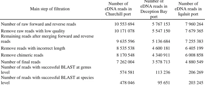
A total of 478,046 aquatic metazoan reads were obtained in Churchill, 95,658 reads in Deception Bay and 203, 245 reads in Iqaluit (see Table S1 for more details about the pipeline
processes). The 18S markers generally generated more sequences than COI markers (with a total of 568 892 and 208 067 sequences respectively), except for in Iqaluit where the reverse situation was observed. In addition, both genetic markers provided distinctive taxonomic resolution according to our knowledge of organisms living in Arctic waters1 (Table 1). The
genus taxonomic level provided a satisfying description of biodiversity given that only 10, 17 and 18% of sequences were not assigned at that this taxonomic level in Churchill, Deception Bay and Iqaluit, respectively (Figure S1). Thus, 2682, 1413 and 1056 operational taxonomic units (OTUs) where identified at the genus level in the ports of Churchill, Deception Bay and Iqaluit, respectively.
Table 1. Summary of the numbers of reads, the proportion of species and genera present in the Arctic historic database and the mean number of OTUs for the COI primers set and the 18S primers set assigned and non assigned on BOLD and SILVA for each port.
Port Number of reads
Proportion of species known in Arctic (%) Proportion of genus known in Arctic (%) Mean nb. of assigned OTUs (genus) Mean nb. of non-assigned OTUs (genus)
COI 18S COI 18S COI 18S COI 18S COI 18S
Churchill 52 749 425 297 52.3 18.7 61.7 45.9 633 708 39 100
Deception
Bay 30 214 65 454 62.9 18.3 74.3 52.6 348 359 16 105
Iqaluit 125 104 78 141 69.4 15.4 77.6 46.3 238 291 4 92
No amplification was observed on agarose gels for the negative PCR controls, but a small number of sequences were present in our laboratory and field negative controls. Two correction factors were applied to ensure the reliability of the data and quality of the resulting analyses. First, the few sequences present in the laboratory negative controls were subtracted
from the samples from the same extraction batch. These sequences represent 0.003%, 0.1% and 0.06% of Churchill, Deception Bay and Iqaluit total number of sequences respectively. Secondly, for the field negative controls, a genus was removed if its abundance in all the field controls was higher than 2% of the total number of sequences for all samples combined for that genus. Following application of correction factors for background contamination, 0.1% and 1.4% of all COI and 18S sequences were removed, respectively (Table S3). An exception to applying correction was made in the case of 18S Pseudocalanus sequences for which 96% of all the field contamination occurred in only one field negative control. Given that
Pseudocalanus in real samples represented nearly half of all 18S sequences and this genus is
known to be a dominant part of the Arctic zooplankton community (Dispas 2019), removing it would cause significant bias to the analyses. When read abundance of a given genus in field controls was lower than 2% of the total number of sequences for that genus, it was retained because contamination was considered low enough that it would not lead to false interpretations. On the contrary, discarding those genera could cause bias in the analyses due to their high number of sequences in real samples.
Arctic coastal gamma diversity
With the exception of benthos communities sampled using trawls, grabs and cores, genera rarefaction curves of marine invertebrates were close to saturation, both for zooplankton surveyed using net tows and eDNA (Figure 2).
Figure 2. Individual-based rarefaction curves of eDNA, benthos and zooplankton genera for Churchill (blue), Deception Bay (yellow) and Iqaluit ports (magenta) based on incidence data. Vertical bars represented 95% confidence intervals.
When eDNA and species collection datasets were combined, a total of 634 marine invertebrate genera from 23 phyla were recorded. Gamma richness was consistently higher for species collections methods than for eDNA, however variable patterns across ports were observed between these sampling approaches. Gamma richness detected with eDNA was higher for Churchill and Deception Bay and lower for Iqaluit port, but the opposite pattern was observed for the gamma richness of communities detected with species collection (Figure 3a). Although a substantial collective number of organisms were detected, few genera where shared between eDNA and species collections (Churchill 15%, Deception Bay 15% and Iqaluit 9%). Of the organisms found with both approaches, annelids accounted for almost half (42.7%), followed by arthropods and molluscs with 20.2% and 11.2% respectively of the common genera obtained within all ports (Figure 3b).
Figure 3. a) Barplots of the number of taxa found in Churchill (blue), Deception Bay (yellow) and Iqaluit (red). Darker bands represent species collection methods while paler bands with dashed outline represent eDNA and black bands represent the number of genera in common between eDNA and species collection. b) Phylum relative proportion of commun genera between eDNA and species collection based on incidence data. COI and 18S primer sets are added together for both a) and b).
The same phyla were generally present among the three ports (Figure 4), with Annelida and
Arthropoda consistently being the most abundant phyla for both eDNA and species
collections. However, for most taxa the relative abundance was significantly different between eDNA and species collection (PERMANOVA, P < 0.001; Table S4; Figure 4). Community composition of eDNA clearly differed among ports (PERMANOVA, P < 0.001;
Table S4; Figure 5a), and this distinction remained significant (PERMANOVA, P < 0.001; Table S4; Figure 5b) for the species collections. Differences in community structure with eDNA versus species collection were mainly driven by annelids and arthropods taxa (SIMPER analysis; 30% and 23% respectively) followed by molluscs, echinoderms, cnidarians and bryozoans (SIMPER analysis; 11%, 6%, 5% and 4% respectively). The remaining differences between eDNA and species collection community compositions may be partly driven by taxa-specific differences in detectability by these approaches. For example, some taxa such as Brachiopoda, Foraminifera, Cephalorhyncha and Chaetognatha (grouped in the Others category with additional phyla of low relative abundance) were only found using species collection, while others such as Bryozoa were only rarely detected using eDNA. In contrast, other taxa such as Porifera, Nemertea, Cnidaria and Echinodermata were more frequently detected with higher read abundances in eDNA samples than in species collections.
Figure 5. Biodiversity differences A) among ports based on eDNA only and B) among sampling methods within ports. Ordination of taxonomic composition (genera) calculated using Sorensen index (incidence based) with each data point representing a specific sample; blue squares represent Churchill, yellow dots represent Deception Bay and magenta triangles represent Iqaluit. Filled symbols are associated with eDNA while empty symbols are associated with species collections.
Alpha biodiversity
Similar to gamma diversity, alpha richness for eDNA samples was significantly higher in Churchill and Deception Bay than Iqaluit (Tukey HSD, p < 0.01), with the number of genera per station ranging from 49 to 75 (mean = 63 ± 2) in Churchill, 45 to 93 (mean = 70 ± 4) in Deception Bay and from 34 to 53 genera (mean = 41 ± 2) in Iqaluit (Figure 6a).
In contrast Churchill had the lowest alpha richness for samples collected using species collection (Tukey HSD, p < 0.01, Figure 6b) with only 8 to 58 genera per station (mean = 27 ± 3) as compared to 30 to 142 (mean = 78 ± 9) and 59 to 151 (mean = 100 ± 8) genera per station in Deception Bay and Iqaluit, respectively. Overall differences between sampling approaches varied between ports, with eDNA-based alpha richness being higher than species collection sample-based richness in Churchill (PERMANOVA, P < 0.001; Table S4), similar in Deception Bay (PERMANOVA, P = 0.4; Table S4), and lower in Iqaluit (PERMANOVA, P < 0.001; Table S4). A similar pattern was also observed with the Shannon biodiversity index (Figure S2).