Energetics of transient-eddy and inter-member variabilities
in global and regional climate model simulations
Oumarou Nikiéma1 · René Laprise1 · Bernard Dugas1
Received: 19 April 2017 / Accepted: 15 September 2017 © The Author(s) 2017. This article is an open access publication
associated with natural phenomena of weather disturbances and IV is a model feature contributing to the uncertainties of simulations.
Keywords Ensemble of climate simulations · Transient eddies · Internal variability · Available enthalpy · Kinetic energy · Atmospheric energy conversions
1 Introduction
Climate models are powerful tools that allow better under-standing of past, present and future climatic phenomena. One advantage that climate models provide is their ability to be used in sensitivity experiments using ensembles of simulations. As first demonstrated by Lorenz (1963) for non-linear systems, climate models exhibit different trajectories in phase space due to their sensitivity to initial conditions (IC).
The study of atmospheric variables using climate models simulations indicates different forms of variability, notably the natural Transient-Eddy (or Time Variability—TV), and Internal (or Inter-member) Variability (IV) when ensembles of simulations are considered. The first form of variability (TV) has a physical meaning since it reflects the passage of weather events (e.g. storms, cyclones, floods, etc.), while the second one (IV) is specific to models and it represents a measure of model’s uncertainties.
Regional Climate Models (RCM) are used to make cli-mate simulations at local scales, but they need to be driven by Lateral Boundary Conditions (LBC) data from reanalysis or low-resolution Global Climate Models (GCM) simula-tions. Over the last two decades, several studies have paid particular attention on RCMs’ IV, e.g. Giorgi and Bi (2000), Weisse et al. (2000) Rinke and Dethloff (2000), Christensen Abstract Available Enthalpy (AE) and Kinetic Energy
(KE) associated with the natural Transient-Eddy (or Time-Variability, TV) and models’ Internal Variability (or Inter-member Variability, IV) are studied using two ensembles of simulations, one from a nested Regional Climate Model (RCM) driven by reanalyses over a regional domain cover-ing eastern North America, and one from a Global Climate Model (GCM), and the Era-interim reanalyses as reference. The fields of TV and IV energies are first examined, both globally and over the regional domain. Results from GCM simulations reveal that GCM TV is similar to that of rea-nalyses, confirming the realism of the GCM simulations, and TV and IV are approximately equal, in agreement with the ergodicity property. For RCM simulations, TV energies are similar to those of reanalyses driving them. On the other hand, the IV energies of reanalyses-driven RCM simulations are much smaller than those of the GCM, because of the control exerted by the lateral boundary conditions imposed in nested models. While GCM IV energies present similar seasonal variations as the TV energies, the RCM IV greatly fluctuates in time, with short episodes of large variations. The second part of this study is devoted to the analysis of TV and IV energetic budgets. Results indicate similar physical interpretations of conversions, generations and destructions for both TV and IV energetics, although TV is
Electronic supplementary material The online version of this article (doi:10.1007/s00382-017-3918-0) contains supplementary material, which is available to authorized users.
* Oumarou Nikiéma [email protected]
1 ESCER Centre, Département des Sciences de la Terre et de
l’Atmosphère, Université du Québec à Montréal (UQAM), Montréal, Canada
O. Nikiéma et al.
et al. (2001), Caya and Biner (2004), Rinke et al. (2004), Lucas-Picher et al. (2004), Alexandru et al. (2007), de Elía et al. (2008) and Lucas-Picher et al. (2008), to name but a few. Recently, Nikiéma and Laprise (2011a, b) have developed a diagnostic approach that furthers our physical understanding of RCM’s IV as a source of uncertainty. They established IV diagnostic equations for different atmospheric variables taking into account the model equations and Reyn-olds’ decomposition applied to the atmospheric field equa-tions, as well as some statistic tools since an ensemble of simulations is considered. Their results suggested a close parallel between the energy conversions associated with the time fluctuations of IV and the TV energy conversions tak-ing place in weather systems as first identified by Lorenz (1955, 1967).
The temperature and the wind are two important dynami-cal atmospheric variables, and they allow defining Poten-tial Energy (PE) and Kinetic Energy (KE). Nowadays, the atmospheric global circulation is well understood following the energy cycle mechanism proposed by Lorenz (1955). He introduced the concept of Available Potential Energy (APE), which is transformed into KE through energy conversions. Indeed, to better understand the role of weather systems in the atmospheric energetics, Lorenz further decomposed the energy fields into components associated with the zonal-mean atmospheric state and departures thereof, termed eddies. Much of our current understanding of global atmos-pheric energetics derives from Lorenz’ seminal work (e.g. Oort 1964a, b; van Mieghem 1973; Newell et al. 1972, 1974; Boer 1974; Pearce 1978); Pexioto and Oort 1992; to name just a few). Following an alternative approach, Marquet (1991, 2003a, b) proposed a formalism based on Available Enthalpy (AE) instead of APE. Inspired by these previous works, Nikiéma and Laprise (2013, 2015) established an approximate energy cycle of IV applicable for a limited-area domain, and afterward adapted to study TV in a particular intense storm observed over the North America (Clément et al. 2016). Their methodology used a decomposition of atmospheric variables into their time-mean state and time variability (perturbations) rather than into zonal-mean and deviations as it is often done for global energetics studies (Lorenz 1955, 1967).
The present study is an extension of previous work with the main goal to compared and analyse AE and KE ener-gies associated with the natural TV and models IV, at global and regional scales. This study is done using three datasets, from ensembles of GCM and RCM simulations, as well as Era-Interim reanalysis considered as reference. Two sets of 50- and 30-member of simulations were performed using the nested fifth-generation Canadian RCM (CRCM5) and it global version (called GEM-Global), respectively. The CRCM5’s simulations were run over a North America regional domain and it was driven by the same LBC from
Era-Interim. For both climate models, all the members were run over the same period and the difference between mem-bers is only the initial data used to start (i.e. IC) each simula-tion. For two consecutive runs, the ICs are the Era-Interim data shifted by 24 h and models output are archived over the same period of interest. The paper is organised as fol-lows: the following Sect. 2 describes the methodology and data used; thereafter, results are presented and discussed in Sect. 3. TV and IV energies are analysed at global and regional scales, as well as energy budgets. Finally, the con-clusion is summarised in Sect. 4.
2 Evaluation methods and data
2.1 Available enthalpy and kinetic energy associated with TV and IV
In an ensemble of N-member simulations, each atmospheric variable 𝜑n, where n represents the simulation’s index, can
be split in two parts: the ensemble-mean noted ⟨𝜑⟩ and the member deviation thereof noted 𝜑�
n = 𝜑n−⟨𝜑⟩. In the same
way for each simulation n, the time deviation over a period of interest can be written as 𝜑��
n = 𝜑n− 𝜑n, where 𝜑n and 𝜑
′′
n
design the time-mean and deviation thereof, respectively. Following Nikiéma and Laprise (2011a, b), the IV for any atmospheric variable 𝜑n can be evaluated by calculating the
inter-member variance 𝜎2
𝜑 as:
The TV can similarly be evaluated as:
where 𝜏 is the number of archive intervals over the period of interest. It is noteworthy that IV is a function of time, unlike TV; hence the time-mean of IV (⟨𝜎2
𝜑
⟩
≡⟨𝜑′2n⟩ )
will be considered in order to compare with TV.
The temperature T and the horizontal wind field
��⃗
V ≡ (U, V) are two important atmospheric variables and
they allow to define Available Enthalpy (EA) and Kinetic Energy (KE) associated with IV (Nikiéma and Laprise 2013) and TV (Clément et al. 2016), calculated as:
(1) 𝜎2 𝜑(i, j, k, t) ≈ 1 N N ∑ n=1 𝜑�2 n(i, j, k, t) ≡ ⟨ 𝜑�2 n ⟩ (2) 2 ∑ 𝜑n (i, j, k) ≈ 1 𝜏 𝜏 ∑ t=1 𝜑��2 n (i, j, k, t) ≡ 𝜑 ��2 n (3) AIV= cp 2Tr ⟨T�2⟩ ≡ cp 2Tr 𝜎2 Tand KIV= 1 2 �→ V� ⋅ → V� � ≡1 2 � 𝜎2 U+ 𝜎 2 V �
Here Tr is a constant reference temperature, which is
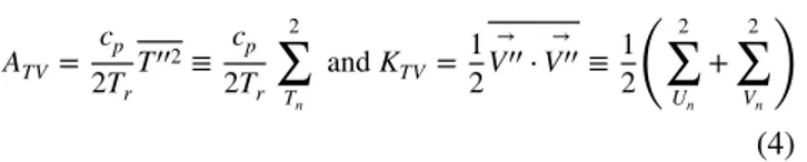
cho-sen so that its inverse corresponds to the inverse of T aver-aged over the time and domain of interest (Marquet 1991). In this study, the reference temperatures will be set to 260°K as in Nikiéma and Laprise (2015) for the same regional domain of interest (eastern North America, see Fig. 1c). It is noteworthy that the formulation of TV energies in Eq. (4) is defined for each simulation n; hence the ensemble-mean of these energies will be considered in order to compare with IV energies. (4) ATV= cp 2Tr T��2≡ cp 2Tr 2 ∑ Tn and KTV = 1 2 → V�� ⋅ → V��≡1 2 ( 2 ∑ Un + 2 ∑ Vn
) 2.2 Ergodicity in climate simulations
One goal of this study is to analyse and compare the sta-tistics of TV and IV energies using GCM and RCM simu-lations. For dynamical systems such as global models of the atmosphere, the ergodic property implies that TV and IV should converge to the same value for a large-member ensemble and over a long time period, i.e.
In the results Sect. 3, TV from Era-interim (Dee et al.
2011) reanalyses will be compared to TV and IV calculated (5) ⟨T�2⟩ ≈ T��2 ⇒AIV ≈ ATV �→ V� ⋅ → V� � ≈ → V�� ⋅ → V��⇒KIV ≈ KTV
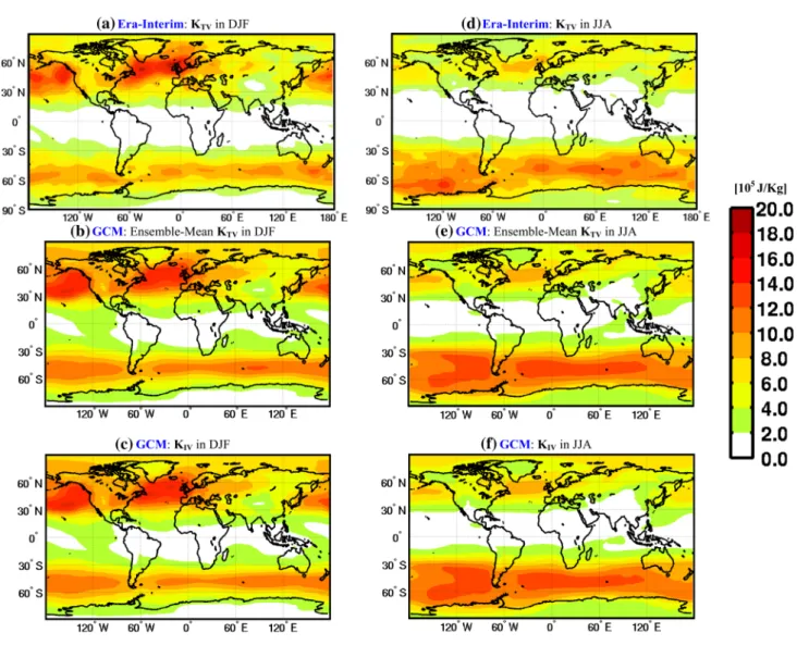
Fig. 1 Maps of vertically integrated available enthalpy associated with transient-eddy variability (ATV) in reanalysis (top row) and
GCM simulations (second row), and associated with inter-member
variability (AIV) in GCM simulations (third row), in DJF (left
col-umn) and JJA (right colcol-umn). The blue rectangle in panel c represents the regional domain of interest. Units: 105 J m2
O. Nikiéma et al.
on simulations ensembles from a reanalyses-driven RCM and from a GCM.
2.3 Budget equations of energies associated with TV and IV
The energy budget equations used in this work were devel-oped in Nikiéma and Laprise (2013) for the IV energy cycle in ensemble of RCM simulations, and in Clément et al. (2016) for the TV energy in a 1-month RCM simulation. As this study focuses on the analysis of the TV and IV vari-abilities, the reservoirs associated with background state, namely time- and ensemble-mean, will not be considered.
Following the above two references, the vari-ability energy prognostic equations (LE = 𝜕E∕𝜕t, with
E∈{AIV, ATV, AIV, ATV}) are written as follows:
where
where l is a factor of order unity factor that depends on the choice of the Tr value, and kIV =
(
U�2+ V�2)/2 and kTV=(U��2+ V��2)/2 are kinetic energies associated with variabilities.
Schematically, the above equations constitute two dif-ferent energy cycles associated with the TV and IV vari-abilities, as shown in Fig. 12. The terms G represent diabatic generation of AE (GTV and GIV) and he terms D relate to the
(6) LA IV = RAIV = CAIV− CIV+ GIV− FAIV − HAIV (7) LK IV = RKIV = CKIV+ CIV− DIV− FKIV− HKIV (8) LA TV = RATV = CATV− CTV+ GTV− FATV− HATV (9) LK TV = RKTV = CKTV+ CTV− DTV− FKTV − HKTV GIV = l⟨T�Q�⟩�T r where l= Tr∕ ⟨T⟩ GTV = lT��Q�� � Tr where l= Tr � T; DIV = − � ���⃗ V� ⋅���⃗F� � ; DTV = −����⃗V�� ⋅����⃗F�� CIV= −⟨𝜔�𝛼�⟩; C TV = −𝜔��𝛼��; CA IV = − Cp Tr �� ���⃗ V�T�� ⋅∇��⃗⟨T⟩ + ⟨𝜔�T�⟩𝜕⟨T⟩𝜕p � ; CA TV = − Cp Tr � ����⃗ V��T�� ⋅∇T + 𝜔��⃗ ��T�� 𝜕T𝜕p � CKIV = − � ���⃗ V�⋅ � ���⃗ V�⋅∇��⃗ �� ��⃗ V �� − � ���⃗ V�⋅ � 𝜔�𝜕 � �⃗ V � 𝜕p �� ; CKTV = −����⃗V��⋅ � ����⃗ V��⋅��⃗∇ � ��⃗ V− ���⃗V�⋅ � 𝜔� 𝜕�⃗V 𝜕p � FAIV = ��⃗∇ ⋅ �� ��⃗ V � AIV � + 𝜕 � ⟨𝜔⟩AIV � 𝜕p ; FATV = ��⃗∇ ⋅ � ��⃗ VATV � + 𝜕(𝜔ATV) 𝜕p FK IV = ��⃗∇ ⋅ �� ��⃗ V � KIV � +𝜕 � ⟨𝜔⟩KIV� 𝜕p ; FKTV = ��⃗∇ ⋅ � ��⃗ VKTV � +𝜕(𝜔KTV) 𝜕p HA IV = Cp 2Tr � ��⃗ ∇ ⋅ � ���⃗ V�T�2�+ 𝜕⟨𝜔�T�2⟩ 𝜕p � ; HA TV = Cp 2Tr � ��⃗ ∇ ⋅ � ����⃗ V��T��2 � + 𝜕𝜔��T��2 𝜕p � HK IV = ��⃗∇ ⋅ �� kIV+ Φ�����⃗V��+𝜕⟨(k+Φ�)𝜔�⟩ 𝜕p ; HKTV = ��⃗∇ ⋅ � kTV+ Φ�������⃗V��+𝜕(k+Φ��)𝜔�� 𝜕p
destruction of KE (DTV and DIV) by dissipation processes.
The terms CA (CATV and CAIV) and CK (CKTV and CKIV) are
conversion terms from the background (time- and ensemble-mean) state to perturbation states for AE and KE, respec-tively. The terms CTV and CIV express the baroclinic energy conversions from AE to KE due to perturbation IV and TV, respectively. The other terms (FE and HE) are boundary flux
terms of energy E, exchanged between the regional domain of interest and the external environment; on a global domain, these terms should vanish, unlike on a regional domain. 2.4 Experiment design and simulations
This study is done using two ensembles of N-member of simulations from a GCM and a RCM, and one dataset from Era-Interim reanalyses (Dee et al. 2011) that is consid-ered as reference and used to drive the RCM. The models used are the fifth-generation Canadian RCM (CRCM5) and its global version referred to as GEM-Global. CRCM5 is based on a limited-area configuration of the GEM3 model (Bélair et al. 2005, 2009) used for numerical weather pre-diction by the Canadian Meteorological Centre (CMC); the land-surface scheme however is the version 3.5 of the Canadian LAnd Surface Scheme (CLASS; Verseghy
2000, 2008). Detailed description of CRCM5 is given in Hernández-Díaz et al. (2013). The RCM and GCM share the same subgrid-scale physical parameterisations, except for slight differences in convection-related formulation to account for differences in resolution. The study of Girard et al. (2014) established that the absence of vertical stag-gering of variables in the discretization of GEM3 induces a computational mode that generates noise near the upper lid
of the model, both in global and regional configurations; enhanced vertical diffusion of the momentum field has often been applied to damp the computational mode near the top of the model. McTaggart-Cowan et al. (2011) also noted the occasional presence of artificial filamentation of the temperature field around the polar vortex near the top of the limited-area version of GEM3; the initial solution to this issue has been to extend the nesting to drive the upper-level temperature field. Recently an alternative fix has been implemented that reduces the problems encoun-tered in both the regional and global versions, consisting in the application of an enhanced horizontal diffusion in the upper levels (currently four levels). Hence there is cur-rently little difference in vertical upper lid of the RCM and GCM used for this study. There is however some enhanced damping applied over the tropical region in the upper part of the GCM domain; but this lies outside the regional focus area of this work.
For all RCM and GCM simulations, sea-surface tempera-ture and sea-ice coverage are prescribed using Era-Interim data after interpolating horizontally to account for the differ-ent grid projection and resolution of RCM and GCM. This reanalysis data is also used as the atmospheric LBC for the RCM, with data linearly interpolated in time at each time step of the RCM. Although CRCM5 code offers the option of large-scale spectral nudging, this option was not used in this study in order to allow the IV to fully develop.
The archived data of the 50-member CRCM5 simula-tions performed by Nikiéma and Laprise (2015) is used. All the RCM simulations were carried out on the same free domain (260 × 160 grid points in the horizontal, excluding the lateral Davies sponge zone and semi-Lagrangian halo), with a grid mesh of 0.3° on a non-rotated latitude-longitude projection, and 56 terrain-following hybrid levels in the vertical. The top level is at about 10 hPa and the timestep is 12 min. Each member starts at 0000 UTC on different days from 12 October to 30 November 2004, for a total of 50 simulations. All the simulations share exactly the same lateral boundary conditions (LBC) from Era-Interim; this means that variability due to different LBC is excluded in this study. The regional domain of study covers the eastern part of North America domain and the adjacent western North Atlantic Ocean, as indicated by the blue rectangle in Fig. 1c.
A set of 30-member GCM simulations have been per-formed. The GCM used a regular latitude-longitude grid of 1° and 64 terrain-following hybrid levels in the vertical, with the top level at 1 hPa, and a timestep of 45 min. The GCM integrations started at 0000 UTC on different days from 12 October to 10 November 2004. Only 30 global simulations were performed due to the limited computational resources; other results show however that 30 members are sufficient to capture most of the IV energy.
For both the RCM and the GCM, the only difference between members is the initial condition used to launch the simulations. The simulations are run for 1 year and the data archived at three hourly intervals, from 1 December 2004 at 0300 UTC to 1 December 2005 at 0000 UTC; but we will focus our analysis on two seasons (DJF and JJA). For the study, the simulated fields are interpolated on 19 pressure levels (1000, 975, 950, 925, 900, 850, 800, 700, 600, 500, 400, 300, 250, 200, 100, 70, 50, 30 and 10 hPa), but we will focus our analysis in the troposphere, i.e. from surface to 250 hPa.
3 Results and analysis
3.1 TV and IV energies at the global scale
Figure 1 shows global maps of vertically integrated values of AE associated with TV (ATV), in DJF (left column) and
JJA (right column), for Era-Interim (top line) and the GCM (second line); the third line shows the corresponding maps of vertically integrated values of AE associated with IV (AIV
) in the 30-member GCM ensemble. Figure 2 shows the cor-responding maps of KTV. For the GCM, ATV and KTV are first
computed for each member in the ensemble of simulations, and the ensemble-mean is shown in Figs. 1 and 2.
The GCM ATV and KTV are found to be similar to those
of the reanalysis, confirming the overall skill of the model at seasonal and global scales. As expected maximum TV is found in middle latitudes, with maximum amplitude in the winter hemisphere where storms are strongest; very weak TV is found in the tropical belt (roughly between 30°S and 30°N). Maximum ATV occurs over North America in DJF,
associated with large thermal contrast between the cold continent and the warm ocean, with values reaching about 8 × 10⁵ J/m2. On the other hand maximum values of K
TV
occur over the oceans, in the circumpolar belt around Ant-arctica and off the East coasts of the North American and Eurasian continents, in association with the strongest storms tracks in the respective winter, with values reaching about 20 × 105 J/m2. Figures 1 and 2 show remarkably similar
pat-terns of IV and TV energies in the GCM simulations, for both AE and KE, confirming that the ergodic property is adequately reproduced with the 30-member GCM ensem-ble. Despite the overall similarities between the ATV and
KTV fields of Era-Interim and GCM simulations,
notewor-thy differences are noted over North America and parts of the Atlantic Ocean in winter, reflecting the different storm tracks.
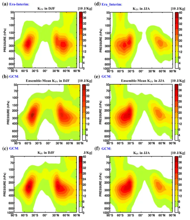
Figures 3 and 4 present corresponding pressure-latitude cross-sections of zonally averaged AE and KE associated with TV and IV, in DJF and JJA. The GCM appears to repro-duce fairly well the TV fields of the reanalysis, and the GCM
O. Nikiéma et al.
TV and IV energies are very similar. Figure 3 shows that AE energies (ATV and AIV) are maximum around 60° of latitude
in both hemisphere, with maximum amplitude in winter; in the vertical three maxima appear, one extending from the surface up to about 500 hPa, another one at the tropopause near 200 hPa, and the third near the top of the displayed domain at 50 hPa. Cross-sections in Fig. 4 indicate that the maximum values of KE (KTV and KIV) are located at around
250 hPa near 45° in the two hemispheres, reflecting large variability associated with the jet stream, with largest ampli-tudes occurring in winter.
3.2 TV and IV energies at the regional scale
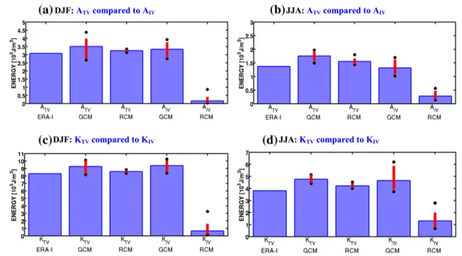
Figure 5 displays histograms of the AE and KE variabili-ties, averaged over the regional domain of interest indi-cated by the blue rectangle in Fig. 1c, integrated over the troposphere from the surface to 250 hPa, and averaged over the 3-month periods of DJF and JJA. The GCM and
RCM values of ATV and KTV are computed for each
mem-ber in the ensembles; the red bar shows the 5–95% percen-tiles range around the mean, and two black dots represent the minimum and maximum values in the ensemble.
The GCM ATV and KTV values are similar to those of
the reanalysis; the RCM values are even closer than those of the GCM owing to the control exerted by the LCB provided by the reanalysis. In DJF, ATV values are about
3.1 × 10⁵, 3.5 × 10⁵ and 3.2 × 10⁵ J/m2 for reanalysis, GCM
and RCM, respectively, and about 1.4 × 10⁵, 1.8 × 10⁵ and
1.6 × 10⁵ J/m2 in JJA. The larger winter values reflect the
important temperature variability over North America. The ATV values can be translated in equivalent temperature
standard deviations of about 4.6, 4.9 and 4.7 K in winter, and 3.0, 3.4 and 3.2 K in summer for reanalysis, GCM and RCM, respectively. The corresponding values of KTV are
about 8.3 × 10⁵, 9.3 × 10⁵ and 8.6 × 10⁵ J/m2 in DJF and
3.8, 4.8 and 4.2 × 10⁵ J/m2 in JJA. Fig. 2 As in Fig. 1, but for kinetic energy transient-eddy variability (KTV) and inter-member variability (KIV)
In the GCM ensemble, results clearly show that IV ener-gies (AIV and KIV) have very similar values to the TV
ener-gies (ATV and KTV) in both seasons. On the other hand, the
RCM IV energies are much smaller than the correspond-ing TV energies, and much smaller than the IV energies of the GCM, owing to the control exerted by the LBC that
are identical for all members in the RCM ensemble. For example, while in DJF, GCM’s AIV and KIV have
intensi-ties of about 3.3 × 10⁵ and 9.4 × 10⁵ J/m2, the RCM’s
val-ues are only 0.2 × 10⁵ and 0.7 × 10⁵ J/m2. Similarly in JJA, AIV ≈ 1.3 × 10⁵ J/m2 and KIV ≈ 4.7 × 10⁵ J/m2 for the GCM
and of AIV ≈ 0.3 × 10⁵ J/m2 and KIV ≈ 1.3 × 10⁵ J/m2 for the
Fig. 3 Pressure-latitude cross sections of zonally averaged available enthalpy associated with transient-eddy variability (ATV) in
reanaly-sis (top row) and GCM simulations (second row), and associated with
inter-member variability (AIV) in GCM simulations (third row), in
O. Nikiéma et al.
RCM. As mentioned in previous studies, such as Alexandru et al. (2007), Lucas-Picher et al. (2004, 2008) and Nikiema and Laprise (2011a, b, 2015), these results confirmed that for RCM’s IV energies the largest values are found in summer over North America compared to those of winter.
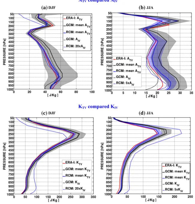
Figure 6 displays the corresponding vertical profiles of variabilities averaged over the regional domain of inter-est indicated by the blue rectangle in Fig. 1c, for AE (top line) and KE (bottom line), in winter (DJF, left column) and
summer (JJA, right column). The profiles of the ensemble-mean TV energies for the GCM and RCM are drawn as black and blue continuous lines, respectively, and the gray and blue shaded bands represent the corresponding range of TV energy values. The IV energies for the GCM and RCM are drawn as black and blue dashed lines, respectively. Reanalysis and GCM and RCM simulations exhibit simi-lar vertical profiles of ATV, with a first maximum near the
surface, around 850–900 hPa, and a second maximum near
150–200 hPa, in both seasons. The profiles of KTV are also
fairly similar for the reanalysis and GCM and RCM simula-tions, exhibiting a single large maximum near the height of the jet stream, around 250 hPa. For both TV energies, the RCM profile is closer to the reanalysis one due to the control exerted by the LBC provided by the reanalysis. As far as the IV energies are concerned, the GCM’s vertical profiles of IV energies are similar to its TV profiles. While the vertical profiles of GCM-simulated ATV and KTV are similar to those
of Era-Interim, we note that the GCM values are generally larger, especially in summer. The RCM IV energies profiles exhibit a similar shape to their TV counterparts, but they are approximately 20 and five times weaker than TV energies in winter and summer, respectively (note the scaling factor applied to RCM IV values).
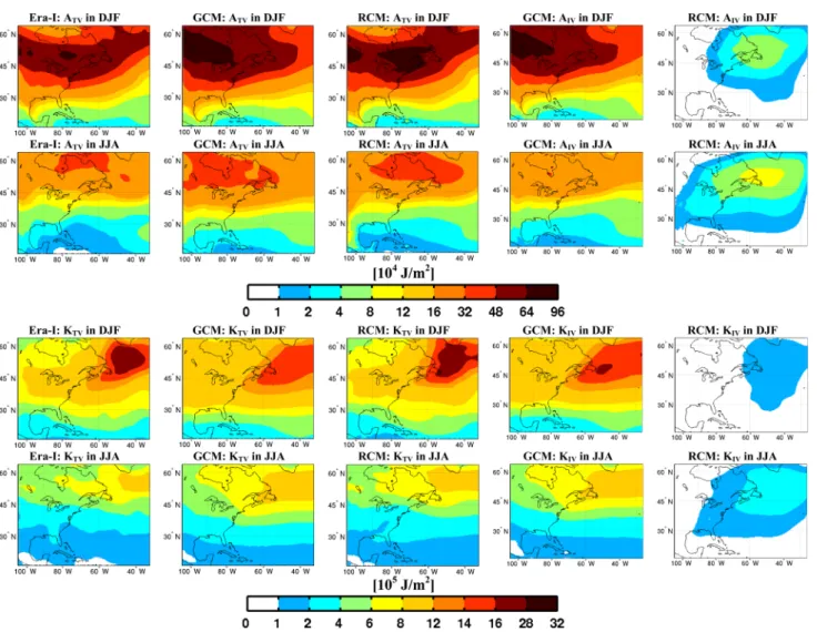
Figure 7 shows the maps of the vertically integrated (from the surface to 250 hPa) fields of ATV, AIV, KTV and
KIV, over the regional domain of interest indicated by the
blue rectangle in Fig. 1c, for the reanalysis, GCM and RCM, in winter and summer (note the different scales used for AE and KE, and for the two seasons). The GCM’s TV results are relatively similar to the reanalysis, confirming the skill of the GCM, but the RCM results are even closer due to the control exerted by the LBC. The GCM’s IV is quite close to the TV values, confirming the ergodicity property. On the other hand, the RCM’s IV is much smaller due to the control exerted by the LBC that imposes vanishing IV at the perim-eter of the domain. The last column in Fig. 7 confirms that
the RCM’s IV energies are transported toward the northeast exit of the regional domain, since the large intensities are found at this location.
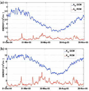
Figure 8 shows the time evolution of the GCM and RCM values of AIV and KIV, averaged over the regional domain and
vertically integrated from the surface to 250 hPa. GCM’s IV energies exhibit a large seasonal variation, with large values in winter and smaller ones in summer, similarly to the afore-mentioned seasonal variations of TV energies. The RCM IV energies are much smaller than those of GCM, they reach their maximum values in summer, and they fluctuate rather erratically in time, with sporadic episodes of large growth quickly followed by equally rapid decay.
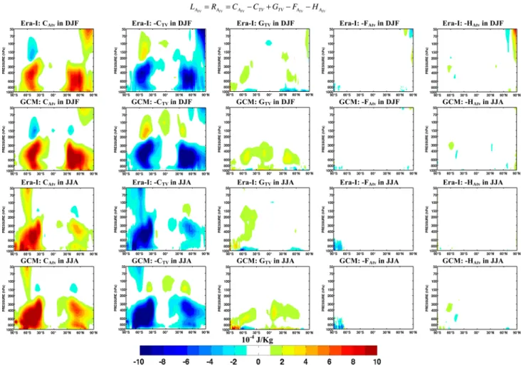
3.3 TV and IV energy budgets at the global scale Figure 9 displays pressure-latitude cross-sections of the zon-ally averaged contributions to ATV tendency RATV (Eq. 8) for
the reanalysis and GCM, in DJF and JJA. For the GCM, the ensemble-mean fields are used. For the reanalysis, the diabatic generation of transient-eddy Available Enthalpy (GTV) is evaluated by calculating the residual values using
the budget equation of ATV (Eq. 8); this probably explains for
a large part the notable differences between the Era-Interim and GCM simulation GTV fields.
In both seasons, and for both reanalysis and GCM, the conversion terms CATV and CATV are much larger than all the
other contributions to the ATV tendency. The conversion
Fig. 5 Average over the domain of interest shown in Fig. 1c of avail-able enthalpy (top row) and kinetic energy (bottom row) associated with transient-eddy variability (subscript TV) and Inter-member Vari-ability (subscript IV), for reanalysis, GCM and RCM simulations, in
DJF (left column) and JJA (right column). IV energies are computed using ensembles of 30 GCM and 50 RCM simulations; the red bar shows the 5–95% percentiles range around the mean, and two black dots represent the minimum and maximum values in the ensemble
O. Nikiéma et al.
terms CATV and CATV almost mirror one another, with
differ-ent signs, indicating a high level of compensation in the ATV
tendency equation: the CATV contributes mostly to increasing ATV while −CTV contributes to decreasing it. Both terms
exhibit maximum intensities in mid-latitudes troposphere and are largest in the winter hemisphere. The GTV
cross-sections (first column in Fig. 9) show weak positive con-tribution to ATV tendency in the middle troposphere, and
weak negative contribution near the surface. In the GCM the
positive contributions are due to condensation and convec-tion processes while the negative contribuconvec-tions near the sur-face are associated with boundary-layer diffusion processes (not shown). The terms FATVand HATV should identically
vanish when integrated over the entire atmosphere. Indeed, Fig. 9 shows that their zonal averages contribute negligibly to the ATV tendency.
Figure 10 shows the corresponding contributions to KTV
tendency RKTV (Eq. 9). For the reanalysis, the term −DTV is
Fig. 6 Vertical profiles of the average over the domain of interest shown in Fig. 1c of available enthalpy (top line) and kinetic energy (bottom line) associated with transient-eddy variability (ATV and
KTV) and inter-member variability (AIV and KIV), for reanalysis,
GCM and RCM, in DJF (left column) and JJA (right column). The
profiles of the ensemble-mean TV energies for the GCM and RCM are drawn as black and blue continuous lines, respectively, and the gray and blue shaded bands represent the corresponding range of TV energy values. The IV energies for the GCM and RCM simulations are drawn as black and blue dashed lines, respectively
evaluated using the estimation of the horizontal momen-tum sources/sinks (�⃗F in term DTV) in the Euler equation. In
general the GCM results are very similar to the reanalysis, except for the terms − DTV that show somewhat larger
dif-ferences due to the fact that they are calculated by residual for the reanalysis. The largest term CTV contributes
posi-tively to KTV tendency, with the largest values in the winter
hemisphere; in the troposphere, this contribution is mostly offset by a negative contribution from the term − HKTV. Near
the surface, the positive contributions of − HKTV are offset
by the dissipation term − DTV. The terms FKTV and HKTV
should identically vanish when integrated over the entire atmosphere; Fig. 10 shows that the zonal average of HATV
has substantial values that exhibit large compensation in the vertical.
Figure 11 shows pressure-latitude cross-sections of the zonally averagedss contributions to AIV tendency RAIV
(Fig. 11a) and KIV tendency RKIV (Fig. 11b) (Eq. 8) for the
GCM, in DJF and JJA. Comparing with corresponding TV fields shown previously in Figs. 9 and 10 confirms very simi-lar results for IV and TV contributions in the 30-member GCM simulations ensemble.
3.4 TV and IV energy budgets at the regional scale In this section, we compare TV and IV energy contribu-tions computed over the regional domain shown as the blue rectangle in Fig. 1c, using data from reanalysis, GCM and RCM. Figure 12 presents each contribution to the AE reser-voirs (ATV or AIV) and KE reservoirs (KTV or KIV), in winter
(Fig. 12a) and summer (Fig. 12b). For GCM and RCM, the ensemble-mean values of contributions in TV energy budg-ets are shown; the red bar shows the 5–95% percentiles range around the mean, and two black dots represent the minimum and maximum values in the ensemble. For a given reservoir,
Fig. 7 Maps of vertically integrated available enthalpy and kinetic energy associated with transient-eddy (ATV and KTV, respectively)
and inter-member variability (AIV and KIV, respectively), for
reanaly-sis, GCM and RCM, in DJF (first and third lines) and JJA (second and fourth lines). Units: 104 J m−2
O. Nikiéma et al.
the ingoing and outgoing arrows indicate the gain and loss of energies, respectively.
Over the regional domain of study, the ATV and AIV
res-ervoirs gain energy mainly by CATV and CAIV and transfer a
similar amount of energy to KTV and KIV via the baroclinic
conversion terms CTV and CIV, respectively. On the other
hand, the KTV and KIV reservoirs loose energy mostly by
the dissipation terms DTV and DIV, but also somewhat by
HK
TV and HKIV, and a little by FKTV and FKIV, respectively. The
three datasets exhibit approximately the same intensity for the transient-eddy fluxes CATV, CTV and DTV, with average
winter values of about 6.4, 6.2 and 3.4 W/m2, and average
summer values of about 2.5, 2.6 and 1.5 W/m2, respectively.
For the GCM, the terms associated with IV have approxi-mately the same intensity to those of TV. The RCM’s IV terms however show much weaker intensities: CAIV = 0.76 W/
m2, C
IV = 0.85 W/m2 and DIV = 0.46 W/m2 in winter, and
CAIV = 1.0 W/m2, CIV = 1.2 W/m2 and DIV = 0.6 W/m2 in
sum-mer. On average, the conversion term CKTV has a small
nega-tive contribution to KTV reservoir for all datasets, as well as
CK
IV for the GCM, while CKIV for the RCM shows a small
positive contribution.
For ATV and AIV reservoirs, the diabatic generation term
(GTV and GIV) and the boundary terms (FATV, HATV and FAIV,
HA
IV) have very small magnitude compared to conversion
terms in both seasons. We can also note that the genera-tion term GTV for the reanalysis, calculated as a residual,
has a different sign than the GCM and RCM in winter and
is close to zero in summer. For KTV and KIV reservoirs, the
boundary terms (FKTV, HKTV and FKIV, HKIV) act to reduce
energies, and the GCM IV contributions are similar to the TV values of the three datasets. The terms FKIV and HKIV for
the RCM, however, are much smaller in winter, but have similar amplitude in summer. Especially in the case of GCM, the large spreads seem to indicate that some mean values are not significant, notably those of FATV and HATV in Fig. 12b
and Fig. 12a, respectively.
Figure 13 displays the vertical profiles of horizontal aver-ages of the terms in the ATV budget in winter (first row)
and summer (second row). The gray and blue light bands represent the ranges of values for terms associated with TV energy tendencies for the GCM and RCM, and their ensemble-mean profiles are shown in black and blue lines, respectively. The profiles of terms in ATV budget for
rea-nalysis are presented in red lines. The profiles of AIV budget
for the GCM and RCM are shown in black and blue dashed lines, respectively.
For terms in ATV budget at the seasonal scale, the results
of the GCM and RCM are generally similar to those of the reanalysis. In terms of intensity, results from climate mod-els (GCM and RCM) and Era-Interim are different for GTV
in both seasons and for conversion terms (CATV and CTV) in
summer. As noted earlier, the term GTV is evaluated by
cal-culating the residual values using the budget equation of ATV
(Eq. 8) for Era-Interim, which could explain the difference of results when compared with ones of climate models. For
CA
TV and CTV in summer, results showed that the covariance
of temperature and wind perturbations from Era-Interim fields are smaller in the troposphere compared to those of climate models (see Fig. 13: second and third bottom panels) resulting to smaller values for reanalysis conversion terms. This result seems to be associated with small values of rea-nalysis’s ATV and KTV in the troposphere during the summer
compared to those of climate models (see Fig. 6b and 6d). The range of values for the RCM terms is smaller than that of the GCM, and it is usually contained within the range of the GCM, except for the term GTV in summer. For the GCM,
the terms in ATV and AIV budgets are rather similar, as seen
by the proximity of the continuous and dashed black lines. For the RCM however the terms in the AIV budget are much
smaller (note the difference of scales), but the vertical pro-files are somewhat similar to those of the ATV budget. The
conversion terms CATV and CAIV act as source for ATV and
AIV reservoirs, which implies that on average covariance of
temperature and wind TV (or IV) fluctuations are down-the-gradient of time- (or -ensemble) mean temperature. The terms − CTV and − CIV act as sink for ATV and AIV
reser-voirs, which implies that temperature and vertical motion TV (or IV) fluctuations are negatively correlated, meaning that warm perturbations rise and cold perturbation sink (e.g., Nikiéma and Laprise 2011a, b, 2015).
Fig. 8 Time evolution of the average over the regional domain of interest shown in Fig. 1c, of inter-member variability available enthalpy (AIV, a) and kinetic energy (KIV, b), in GCM and RCM
In winter, the diabatic generation term GTV contributes
positively between 250 and 850 hPa and negatively in the lower layers (between 850 hPa and surface) for all the data-sets, as well as GIV for the GCM and RCM. The
reanal-ysis profile is similar to that of models, but with weaker positive contribution in the middle troposphere and larger negative contribution near the surface. In summer, the two climate models indicate positive contribution of GTV at all
pressure levels, on average, and results from the reanalysis show positive and negative contributions in higher (above 650 hPa) and lower troposphere, respectively. Physically, the positive sign of terms G means that temperatures TV (or IV) perturbations are positive correlated with diabatic heating perturbations associated with condensation, convection and radiation processes (results not shown); their negative sign near the surface reflect boundary-layer turbulent diffusion processes (results not shown).
The vertical profiles of boundary terms (F and H) of ATV
tendency show weak contributions with positive and nega-tive values ranged between ±1 × 10⁻⁴ W/kg, as well as A
IV
tendency for the GCM. For the RCM, the range of values is
about five times smaller. For the RCM, the term FAIV
con-tributes negatively at all pressure levels and in both seasons because AIV energy is transported out of the regional domain
(e.g. Nikiéma and Laprise 2011a, b, 2015).
Figure 14 shows the corresponding vertical profiles of horizontally averaged contributions to KTV and KIV
budg-ets, using the same colour convention. In general the TV results of the models are similar to those of the reanalysis, with a larger ranges of values for the GCM than the RCM. The KTV and KIV reservoirs are fed mainly by the baroclinic
conversion terms CTV and CIV, respectively, which are offset
by negative contribution of − HKTV and − HKIV in the
mid-dle troposphere, and by the dissipation processes − DTV and
−DIV near the surface as a result of Ekman pumping (e.g.
Nikiéma and Laprise 2015). The boundary terms − FKTV and
− FKIV act mostly negatively, with largest values in the
vicin-ity of the tropopause near the jet stream, as a result of TV or IV kinetic energies being transported outside the regional domain. At the regional scale, the term CKTV < 0 implies
that the KTV energy contributes to reinforce the background
kinetic energy mostly near the jet stream.
Fig. 9 Pressure-latitude cross-sections of the zonally averaged contributions to the transient-eddy Available Enthalpy (ATV) tendency (RATV) for
O. Nikiéma et al.
For the GCM, the IV results are similar to those of the TV. For the RCM, the IV terms have smaller intensity but exhibit generally similar profiles to those of the TV, except for the barotropic conversion term (CKIV > 0) that has
posi-tive sign, contrary to GCM’s result. This result indicates that this term (CKIV) acts to feed KIV reservoir from the
ensemble-mean kinetic energy (Nikiema and Laprise 2015), unlike the case of the GCM where the ensemble-mean kinetic energy is fed by CKIV.
In the following paragraphs of this section, the reader is referred to Figures S1 and S2 in the Supplementary Mate-rial. Figure S1 displays the maps of contributions, vertically integrated over the whole troposphere (from the surface to 250 hPa), of all the terms in the ATV budget for the
rea-nalysis, the GCM and RCM, and in the AIV budget for the
GCM and RCM, in winter (panel S1a) and summer (panel S1b); note that different scaling used for some terms. For the climate models, the ATV ensemble-mean contributions
are shown.
For the ATV contributions we note again that, while the
GCM’s contributions are somewhat similar to those of the reanalysis, the RCM’s contributions are very close to those
of the reanalysis due to the control exerted by the LBC. On the other hand the GCM’s AIV contributions are very similar
to those of the ATV contributions, reflecting the ergodicity
property. Hence the patterns of each IV and TV contribu-tions are similar for all datasets, except for the RCM’s AIV
contributions.
In all datasets, there are large compensating contributions from terms CATV and CTV to the ATV budget, with maximum
intensity of about 30 W/m2 along the storm tracks off the
east coast in winter, and 10 W/m2 over Canada in summer.
For the GCM, the patterns of these conversions terms are similar to those of CAIV and CIV in the AIV budget. In the
RCM, while the CAIV and CIV terms are also largely
compen-sating one another, their patterns are rather different from the corresponding TV terms, reaching their maximum inten-sity near the northeastern (outflow) part of the domain, with maximum intensities of only about 3 W/m2.
The diabatic generation term GTV is modest, with
maxi-mum values of about 3 W/m2 in both seasons. In the
rea-nalysis this term is computed as residual, which may explain why its pattern is very noisy and rather different from that of the climate models. There is however a general common
characteristic of being mainly positive over the continent and negative over the ocean in winter.
It was noted earlier that the boundary-flux term −FATV
and the third-order term −HATV have weak magnitudes when
averaged over the domain (Fig. 12); these fields however exhibit locally non-negligible values in the three datasets. In the GCM these terms are also similar to the patterns of −HAIV and −FAIV. In the RCM, the terms −HAIV and −FAIV are
rather negligible, but we note that −FAIV reflects the fact that AIV energy is transported out of the regional domain by the
mean flow.
The three datasets exhibit similar horizontal pattern of −HKTV, with dominant negative values resulting from values
in the middle troposphere (from 250 to 850 hPa), only partly offset by values of opposite sign below 850 hPa, as seen in Fig. 14. Similar results are also seen for −HKIV in the GCM,
while RCM values are much smaller and exhibit different pattern.
The last row in Figure S2 displays the contribution −FKTV
for the three datasets, and −FKIV for the two climate models.
All the maps show mainly negative values mostly over the eastern part of Canada, indicating that KTV and KIV loose
energy by their transport outside this specific regional domain.
4 Discussion and conclusion
We compared the energetics of Available Enthalpy (AE) and Kinetic Energy (KE) transient-eddy variability (TV) and inter-member variability (IV) from two ensembles of simulations, one from a Global Climate Model (GCM) and one from a Regional Climate Model (RCM) integrated over an eastern North American domain. The models’ TV statis-tics were compared to those of the Era-Interim reanalysis, considered here as the reference. The 30 GCM members and 50 RCM members simulations were initialised from the reanalysis, starting on different dates shifted by 24 h from 12 October 2004 at 0000 UTC, and were run till the 31 December 2005, using the sea-surface conditions from the
Fig. 11 Pressure-latitude cross-sections of the zonally averaged contributions to the GCM inter-member variability available enthalpy (AIV)
reanalysis. All the members in the RCM simulations used the same lateral boundary conditions (LBC) from reanaly-ses, which limits IV due to the control exerted by the LBC in nested models. The study focussed on the two solstice sea-sons, December 2004–January 2005–February 2005 (noted DJF) and June–July–August of 2005 (noted JJA).
In the reanalysis, transient-eddy Available Enthalpy and Kinetic Energy (ATV and KTV, respectively) are found mostly
near the storm track over mid-latitudes in both hemispheres. The maximum values of ATV are especially intense over
North America in winter, indicating that this region is sub-ject to large variations of temperature. The vertical distribu-tion of the zonally averaged KTV shows that the maximum is
associated with wind fluctuations in the jet stream near the tropopause in mid-latitudes. The GCM transient-eddy sta-tistics are similar to those of the reanalysis; the spread of the
transient-eddy statistics in the 30-member GCM ensemble is quite large, and in most cases encompasses the reanalysis values, confirming the skill of the GCM. Over the North American regional domain, the RCM’s transient-eddy statis-tics are very similar to the reanalysis ones (in fact closer than the GCM), and the spread of the transient-eddy statistics in the 50-member RCM ensemble is much smaller than that in the GCM ensemble, owing to the control exerted upon the RCM simulations by the LBC provided by the reanalysis.
In the GCM simulations, the statistics of inter-member variability are very similar to those of transient-eddy vari-ability, in agreement with the ergodicity property. The situ-ation is quite different for the RCM simulsitu-ations where the inter-member variability is much lesser and vanishes near the perimeter of the regional domain due to the control exerted by LBC that are identical for all members in the ensemble. Over North America the GCM’s inter-member variability undergoes an annual cycle that reflects the ampli-tude of transient eddies, with maximum/minimum intensity occurring in winter/summer. The RCM’s inter-member vari-ability however has much weaker amplitude and it exhibits brisk fluctuations, with episodes of large growth followed by rapid decay within a few days. Furthermore, large values of IV energies are found in summer for RCM because of
Fig. 12 (continued)
Fig. 12 Energy cycles associated with transient-eddy (ATV and KTV,
respectively) and inter-member variability (AIV and KIV,
respec-tively), for reanalysis, GCM and RCM simulations, in DJF (a) and JJA (b), averaged over the regional domain shown as the blue rec-tangle in Fig. 1c. For GCM and RCM, the ensemble-mean values of contributions in TV energy budgets are shown; the red bar shows the 5–95% percentiles range around the mean, and the red dots represent the minimum and maximum values in the ensemble
O. Nikiéma et al.
Fig. 13 Vertical profiles of horizontally averaged contributions in the budget equations of transient-eddy and inter-member variability avail-able enthalpy (ATV and AIV, respectively), for reanalysis, GCM and RCM simulations, in DJF (first row) and JJA (second row). The gray and blue light bands represent the ranges of values for terms
associ-ated with TV energy tendencies for the GCM and RCM, respectively, and their ensemble-mean profiles are shown in black and blue lines, respectively. The profiles of terms in ATV budget for reanalysis are presented in red lines. The profiles of AIV budget for the GCM and RCM are shown in black and blue dashed lines, respectively
stronger local processes, such as condensation and convec-tion, while in winter the stronger advection of IV energy out of the domain lead to a weak IV energy.
This study also analysed the energetics of AE and KE res-ervoirs associated with transient-eddy variability (ATV and
KTV) and inter-member variability (AIV and KIV). Together
these two energies (AE and KE) constitute a cycle with conversion of energy from one to the other. At the global scale, transient-eddy energetics budgets from reanalysis and GCM are quite similar and, in the GCM, the inter-member variability energetics are quite similar to those of transient eddies. The results indicate that the most important pertur-bation energy exchanges operate over the mid-latitudes in the troposphere.
Over the North American domain, the energetics of the GCM simulations and reanalysis are quite similar, as well as RCM’s simulation TV energetics. Energy is supplied to the transient-eddy available enthalpy (ATV) reservoir mainly by
the term CATV that converts available enthalpy from its
time-mean state to transient eddies. This conversion term is maxi-mum in mid-latitudes where weather systems transport heat poleward through covariance of temperature and wind per-turbations (����⃗V′′T′′) down-the-gradient of time-mean
tempera-ture field (��⃗∇T). The term CTV transfers energy from
tran-sient-eddy available enthalpy (ATV) to transient-eddy kinetic
energy (KTV) through baroclinic conversion, with warm/cold
air rising/sinking on average in mid-latitude weather sys-tems, due to covariance of temperature and vertical motion perturbations (𝜔′′𝛼′′). Transient-eddy kinetic energy is lost
mainly through two physical processes: dissipation (DTV)
and transport outside the regional domain (FKTV). In the
plan-etary boundary layer where the dissipation processes are important, results indicate that the term DTV is partly offset
by the vertical component of the boundary term −HKIV
because of Ekman pumping (−𝜕 𝜕pΦ
��𝜔��> 0). For example,
in a low-pressure system (��< 0), warm air near the surface
is forced to rise due to friction-induced convergence (𝜔��< 0), leading to a positive covariance of fluctuations
(Φ��𝜔��> 0); negative vertical variation of the covariance
(𝜕
𝜕pΦ��𝜔��< 0) follows because covariance increases with
height in low levels.
The analysis of the GCM simulations ensemble reveals that the energetics of inter-member variability is very similar to that of transient eddies, again confirming the ergodicity property of GCM ensembles. It is most interest-ing that IV and TV energy cycles share the same physical interpretation, with for example “baroclinic” conversion
CIV occurring for notional inter-member perturbations just
as it does through CTV for actual transient eddies in weather
systems. The RCM simulations ensemble on the other hand exhibits much weaker inter-member variability energy and conversion intensity compared to those of GCM, which
makes sense due to the control exerted by LBC that are identical for all members in the RCM ensemble. It is note-worthy that IV conversions occur in the RCM ensemble similar to those in the GCM ensemble, but with reduced amplitude, leading to similar physical interpretations for most of the terms in the budget; one main difference is the importance of the inter-member variability export out of the RCM domain. Despite the fact that inter-member variability is often considered a source of uncertainty for climate models, the present study confirms that it arises from the chaotic nature of the atmosphere and that it is not associated with numerical artefact, in particular, in the case of nested models.
Acknowledgements This research was co-funded by the Climate Change and Atmospheric Research (CCAR) programme of the Natu-ral Sciences and Engineering Research Council of Canada (NSERC) through a grant to the “Canadian Network for Regional Climate and Weather Processes” (CNRCWP; http://www.cnrcwp.uqam.ca), by the project “Marine Environmental Observation, Prediction and Response” (MEOPAR; http://meopar.ca) of the Canadian Networks of Centres of Excellence, and by the NSERC Discovery Accelerator Supplements Program. The calculations were made on the Guillimin supercomputer of Compute Canada - Calcul Québec whose operation is funded by the Canada Foundation for Innovation (CFI), NanoQuébec, RMGA and the Fonds de recherche du Québec—Nature et technologies (FRQ-NT). The authors thank Mr. Georges Huard and Mrs. Nadjet Labassi and Mrs. Katja Winger for maintaining an efficient and user-friendly local computing facility.
Open Access This article is distributed under the terms of the Creative Commons Attribution 4.0 International License ( http://crea-tivecommons.org/licenses/by/4.0/), which permits unrestricted use, distribution, and reproduction in any medium, provided you give appro-priate credit to the original author(s) and the source, provide a link to the Creative Commons license, and indicate if changes were made.
References
Alexandru A, de Elia R, Laprise R (2007) Internal Variability in regional climate downscaling at the seasonal scale. Mon Weather Rev 135:3221–3238
Bélair S, Mailhot J, Girard C, Vaillancourt P (2005) Boundary-layer and shallow cumulus clouds in a medium-range forecast of a large-scale weather system. Mon Weather Rev 133:1938–1960 Bélair S, Roch M, Leduc AM, Vaillancourt PA, Laroche S, Mailhot J
(2009) Medium-range quantitative precipitation forecasts from Canada’s new 33-km deterministic global operational system. Weather Forecast 24:690–708. doi:10.1175/2008WAF2222175.1
Boer GJ (1974) Zonal and eddy forms of the available potential energy equations in pressure coordinates. Tellus 27(5):433–442 Caya D, Biner S (2004) Internal variability of RCM simulations over
an annual cycle. Clim Dyn 22:33–46
Christensen OB, Gaertner MA, Prego JA, Polcher J (2001) Internal variability of regional climate models. Clim Dyn 17:875–887 Clément M, Nikiéma O, Laprise R (2016) Limited-area atmospheric
energetics: illustration on a simulation of the CRCM5 over east-ern North America for December 2004. Clim Dyn. doi:10.1007/ s00382-016-3198-0
O. Nikiéma et al. de Elía R, Caya D, Côté H, Frigon A, Biner S, Giguère M, Paquin D,
Harvey R, Plummer D (2008) Evaluation of uncertainties in the CRCM-simulated North American climate. Clim Dyn 30:113– 132. doi:10.1007/s00382-007-0288-z
Dee DP, Uppala SM, Simmons AJ, Berrisford P, Poli P, Kobayashi S, Andrae U, Balmaseda MA, Balsamo G, Bauer P (2011) The ERA-Interim reanalysis: configuration and performance of the data assimilation system. Q J R Meteorol Soc 137:553–597. doi:10.1002/qj.828
Giorgi F, Bi X (2000) A study of internal variability of regional climate model. J Geophys Res 105:29503–29521
Girard C, Plante A, Desgagné M, McTaggart-Cowan R, Côté J, Charron M, Gravel S, Lee V, Patoine A, Qaddouri A, Roch M, Spacek L, Tanguay M, Vaillancourt PA, Zadra A (2014) Stag-gered vertical discretization of the Canadian environmental mul-tiscale (GEM) model using a coordinate of the log-hydrostatic-pressure type. Mon Weather Rev 142:1183–1196. doi:10.1175/ MWR-D-13-00255.1
Hernández-Díaz L, Laprise R, Sushama L, Martynov A, Winger K, Dugas B (2013) Climate simulation over CORDEX Africa domain using the fifth-generation Canadian regional climate model (CRCM5). Clim Dyn 40(5–6):1415–1433. doi:10.1007/ s00382-012-1387-z
Lorenz EN (1955) Available potential energy and the maintenance of the general circulation. Tellus 7:157–167
Lorenz EN (1963) Deterministic non-periodic flow. J Atmos Sci 42:433–471
Lorenz EN (1967) The nature and theory of the general circulation of the atmosphere. WorldMeteorol Organ 218 TP 115:161
Lucas-Picher P, Caya D, Biner S (2004) RCM’s internal variability as function of domain size. Research activities in atmospheric and oceanic modelling, WMO/TD. J Côté Ed 1220 34:7.27–7.28 Lucas-Picher P, Caya D, de Elía R, Laprise R (2008) Investigation of
regional climate models’internal variability with a ten-member ensemble of 10-year simulations over a large domain. Clim Dyn 31:927–940. doi:10.1007/s00382-008-0384-8
Marquet P (1991) On the concept of energy and available enthalpy: application to atmospheric energetics. Q J R Meteorol Soc 117:449–475
Marquet P (2003a) The available-enthalpy cycle. I: Introduction and basic equations. Q J R Meteorol Soc 129(593):2445–2466 Marquet P (2003b) The available-enthalpy cycle. II:
Applica-tions to idealized baroclinic waves. Q J R Meteorol Soc 129(593):2467–2494
McTaggart-Cowan R, Girard C, Plante A, Desgagné M (2011) The utility of upper-boundary nesting in NWP. Mon Weather Rev 139:2117–2144. doi:10.1175/2010MWR3633.1
Newell RE, Kidson JW, Vincent DG, Boer GJ (1972) The general cir-culation of the tropical atmosphere and interactions with extrat-ropical latitudes. MIT Press, vol 1, p. 320
Newell RE, Kidson JW, Vincent DG, Boer GJ (1974) The general cir-culationof the tropical atmosphere and interactions with extrat-ropical latitudes. MIT Press, vol 2, p 370
Nikiéma O, Laprise R (2011a) Diagnostic budget study of the internal variability in ensemble simulations of the Canadian RCM. Clim Dyn 36(11):2313–2337. doi:10.1007/s00382-010-0834-y
Nikiéma O, Laprise R (2011b) Budget study of the internal variability in ensemble simulations of the Canadian RCM at the seasonal scale. J Geophys Res Atmos. doi:10.1029/2011JD015841
Nikiéma O, Laprise R (2013) An approximate energy cycle for inter-member variability in ensemble simulations of a regional climate model. Clim Dyn 44(3–4):831–852. doi:10.1007/ s00382-012-1575-x
Nikiéma O, Laprise R (2015) Energy cycle associated with inter-mem-ber variability in a large ensemble of simulations with the Cana-dian RCM (CRCM5). Clim Dyn. doi:10.1007/s00382-015-2604-3
Oort AH (1964a) On estimates of the atmospheric energy cycle. Mon Weather Rev 92:483–493
Oort AH (1964b) On the energetics of the mean and eddy circulations in the lower stratosphere. Tellus 26(3):309–327
Pearce RP (1978) On the concept of available potential energy. Q J R Meteorol Soc 104:737–755
Rinke A, Dethloff K (2000) On the sensitivity of a regional Arctic climate model to initial and boundary conditions. Clim Res 14:101–113
Rinke A, Marbaix P, Dethloff K (2004) Internal variability in Arctic regional climate simulations: case study for the SHEBA year. Clim Res 27:197–209
van Mieghem J (1973) Atmospheric energetics. Oxford Univ Press Verseghy LD (2000) The Canadian land surface scheme (CLASS): its
history and future. Atmos Ocean 38:1–13
Verseghy LD (2008) The Canadian land surface scheme: technical documentation—version 3.4. ClimateResearch Division, Science and Technology Branch, Environment Canada
Weisse R, Heyen H, von Storch H (2000) Sensitivity of a regional atmospheric model to a sea state dependent roughness and the need of ensemble calculations. Mon Weather Rev 128:3631–3642