UCD : Upper Confidence bound for rooted Directed
acyclic graphs
Abdallah Saffidinea, Tristan Cazenavea, Jean Méhatb
aLAMSADE Université Paris-Dauphine Paris, France bLIASD Université Paris 8 Saint-Denis France Abstract
In this paper we present a framework for testing various algorithms that deal with transpositions in Monte-Carlo Tree Search (MCTS). We call this framework Upper Confidence bound for Direct acyclic graph (UCD) as it constitutes an extension of Upper Confidence bound for Trees (UCT) for Direct Acyclic Graph (DAG).
When using transpositions in MCTS, a DAG is progressively developed instead of a tree. There are multiple ways to handle the exploration exploita-tion dilemma when dealing with transposiexploita-tions. We propose parameterized ways to compute the mean of the child, the playouts of the parent and the playouts of the child. We test the resulting algorithms on several games. For all games, original configurations of our algorithms improve on state of the art algorithms.
Keywords: Monte-Carlo Tree Search, UCT, Transpositions, DAG
1. Introduction
Monte-Carlo Tree Search (MCTS) is a very successful algorithm for multi-ple commulti-plete information games such as Go [1, 2, 3, 4, 5], Hex [6, 7], or Lines of
Email addresses: [email protected] (Abdallah Saffidine), [email protected] (Tristan Cazenave), [email protected] (Jean Méhat)
Action [8]. Monte-Carlo programs usually deal with transpositions the sim-ple way: they do not modify the Upper Confidence bound for Trees (UCT) formula and develop a Direct Acyclic Graph (DAG) instead of a tree.
Transpositions are widely used in combination with the Alpha-Beta al-gorithm [9] and they are a crucial optimisation for games such as Chess. Transpositions are also used in combination with the MCTS algorithm but little work has been done to improve their use or even to show they are use-ful. The only works we are aware of are the paper by Childs et al. [10] and the paper by Méhat and Cazenave [11].
Our main contribution consists in providing a parametric formula adapted from the UCT formula 2 so that some transpositions are taken into account. Our framework encompasses the work presented in [10]. We show that the simple way is often surpassed by other parameter settings on an artificial one player game as well as on the two player games hex and go as well as several games from General Game Playing competitions. We do not have a definitive explanation on how parameters influence the playing strength yet. We show that storing aggregations of the payoffs on the edge rather than on the nodes is preferable from a conceptual point of view and our experiment show that it also often lead to better results.
The rest of this article is organised as follows. We first recall the most common way of handling transpositions in the MCTS context. We study the possible adaptation of the backpropagation mechanism to DAG game trees. We present a parametric framework to define an adapted score and an adapted exploration factor of a move in the game tree. We then show that our framework is general enough to encompass the existing tools for transpositions in MCTS. Finally, experimental results on an artificial single player game and on several two players games are presented.
2. Motivation
We will use the following notations for a given object x. If x is a node, then c(x) is the set of the edges going out of x, similarly if x is an edge and y is its destination, then c(x) = c(y) is the set of the edges going out y. We indulge in saying that c(x) is the set of children of x even when x is an edge. If x is an edge and y is its origin, then b(x) = c(y) is the set of edges going out of y. b(x) is the set of the “siblings” of x plus x. During the backpropagation step, payoffs are cumulatively attached to nodes or edges. We denote by µ(x) the mean of payoffs attached to x (be it an edge or a
node), and by n(x) the number of payoffs attached to x. If x is an edge and y is its origin, we denote by p(x) the total number of payoffs the children of y have received: p(x) = P
e∈c(y)n(e) =
P
e∈b(x)n(e). Let x be a node or an
edge, between the apparition of x in the tree and the first apparition of a child of x, some payoffs (usually one) are attached to x, we denote the mean (resp. the number) of such payoffs by µ0(x) (resp. n0(x)). We denote by π(x) the best move in x according to a context dependant policy.
Before having a look at transpositions in the MCTS framework, we first use the notation to express a few remarks on the plain UCT algorithm (when there is no transpositions). The following equalities are either part of the definition of the UCT algorithm or can easily be deduced. The payoffs available at a node or an edge x are exactly those available at the chil-dren of x and those that were obtained before the creation of the first child: n(x) = n0(x) +P
e∈c(x)n(e). The mean of a move is equal to the weighted
mean of the means of the children moves and the payoffs carried before cre-ation of the first child:
µ(x) = µ
0(x) × n0(x) +P
e∈c(x)µ(e) × n(e)
n0+P
e∈c(x)n(e)
(1)
The plain UCT value [12] with an exploration constant c giving the score of a node x is written
u(x) = µ(x) + c × s
log p(x)
n(x) (2)
The plain UCT policy consists in selecting the move with the highest UCT formula: π(x) = maxe∈c(x)u(e). When enough simulations are run at
x, the mean of x and the mean of the best child of x are converging towards the same value [12]:
lim
n(x)→∞µ(x) =n(x)→∞lim µ(π(x)) (3)
Introducing transpositions in MCTS is challenging for several reasons. First, equation 1 may not hold anymore since the children moves might be simulated through other paths. Second, UCT is based on the principle that the best moves will be chosen more than the other moves and consequently the mean of a node will converge towards the mean of its best child; hav-ing equation 1 holdhav-ing is not sufficient as demonstrated by Figure 1 where equation 3 is not satisfied.
µ = .5 n = 2 µ = .4 n = 2 µ = .5 n = 2 µ = .5 n = 2 µ = .45 n = 4 E = .8 E = .5
(a) Initial settings
µ = .5 n = 102 µ = .4 n = 2 µ = .5 n = 102 µ = .5 n = 102 µ = .498 n = 104 E = .8 E = .5 (b) 100 playouts later
Figure 1: Counter-example for the update-all backpropagation procedure. If the initial estimation of the edges is imperfect, the UCT policy combined with the update-all back-propagation procedure is likely to lead to errors.
Suppose we have a single-player graph of size 5 as depicted in Figure 1 (a), with two leaves such that the leaf on the left is deterministic (or has a very low variance) and the associated reward is 0.5, and the leaf on the right is non-deterministic with mean reward 0.8. The best policy from the root for a risk neutral agent is to select the right edge twice and arrive at the 0.8 leaf. We will show that using the UCT policy together with the update-all backpropagation mechanism and show that it does not to lead to selecting the correct action sequence. Assume that the algorithm started by selecting twice the 0.5 leaf and twice the 0.8 leaf but that the mean of the results for the 0.8 leaf is 0.4. We obtain the situation depicted in Figure 1 (a). As we can see from the root, the left edge has a higher mean and a higher exploration value that the right edge. As a result the UCT policy will select the left edge ending invariably in the 0.5 leaf. The update-all backpropagation will update the µ and n values of both edges from the root, but the left edge will keep a higher mean and a higher exploration value. Figure 1 (b) shows the situation after 100 more descents of the algorithm. The UCT policy and the update-all procedure are such that every descent ended selecting the left 0.5 leaf. As a consequence, if the mean of the first draws on the 0.8 leaf are lower than 0.5, the UCT policy together with the update-all procedure will no select the right action to start with, no matter the number of descents performed.
frame-work, beside ignoring them completely, is what will be referred to in this article as the simple way. Each position encountered during the descent cor-responds to a unique node. The nodes are stored in hash-table with the key being the hash value of the corresponding position. Mean payoff and number of simulations that traversed a node during the descent are stored in that node. The plain UCT policy is used to select nodes.
The simple way shares more information than ignoring transpositions. Indeed, the score of every playout generated after a given position a is aggre-gated in the node representing a. On the other hand, when transpositions are not detected, playouts generated after a position a are divided among all nodes representing a in the tree depending on the moves at the beginning of the playouts.
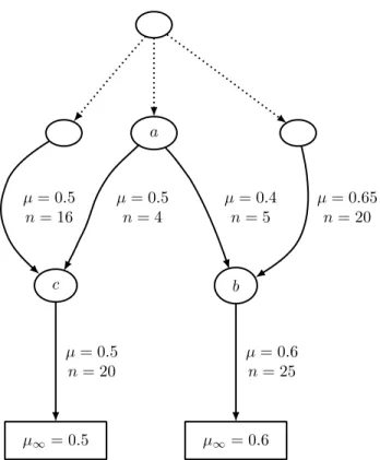
It is desirable to maximise the usage of a given amount of information because it allows to make better informed decisions. In the MCTS context, information is in the form of playouts. If a playout is to be maximally used, it may be necessary to have its payoff available outside of the path it took in the game tree. For instance in Figure 2 the information provided by the playouts were only propagated on the edges of the path they took. There is not enough information directly available at a even though a sufficient number of playouts has been run to assert that b is a better position than c. Nevertheless, it is not trivial to share the maximum amount of informa-tion. A simple idea is to keep the DAG structure of the underlying graph and to directly propagate the outcome of a playout on every possible ancestor path. It is not always a good idea to do so in a UCT setting, as demonstrated by the counter-example in Figure 1. We will further study this idea under the name update-all in Section 3.2.
3. Possible Adaptations of UCT to Transpositions
The first requirement of using transpositions is to keep the DAG structure of the partial game tree. The partial game tree is composed of nodes and edges, since we are not concerned with memory issues in this first approach, it is safe to assume that it is easy to access the outgoing edges as well as the in edges of given nodes. When a transposition occurs, the subtree of the involved node is not duplicated. Since we keep the game structure, each possible position corresponds to at most one node in the DAG and each node in the DAG corresponds to exactly one possible position in the game. We will indulge ourselves to identify a node and the corresponding position. We
µ = 0.5 n = 20 µ = 0.4 n = 5 µ = 0.6 n = 25 µ = 0.5 n = 16 µ = 0.65 n = 20 µ = 0.5 n = 4 a µ∞= 0.6 b µ∞= 0.5 c
Figure 2: There is enough information in the game tree to know that positionb is better than position c, but there is not enough local information at node a to make the right decision.
will also continue to call the graph made by the nodes and the moves game tree even though it is now a DAG.
3.1. Storing results in the edges rather than in the nodes
In order to descend the game tree, one has to select moves from the root position until reaching an end of the game-tree. The selection uses the results of the previous playouts which need to be attached to moves. A move corresponds exactly to an edge of the game tree, however it is also possible to attach the results to nodes of the game tree. When the game tree is a tree, there is a one to one correspondence between edges and nodes, save for the root node. To each node but the root, correspond a unique parent edge and each edge has of course a unique destination. It is therefore equivalent to attach information to an edge (a, b) or to the destination b of that edge. MCTS implementations seem to prefer attaching information to nodes rather than to edges for implementation simplicity reasons. When the game tree is a DAG, we do not have this one to one correspondence so there may be a difference between attaching information to nodes or to edges.
In the following we will assume that aggregations of the payoffs are at-tached to the edges of the DAG rather than to the nodes. The payoffs of a node a can still be accessed by aggregating the payoffs of the edges arriving in a. No edge arrives at the root node but the results at the root node are usually not needed. On the other hand, the payoffs of an edge cannot be easily obtained from the payoffs of its starting node and its ending node, therefore storing the results in the edges is more general than storing the results only in the nodes.1
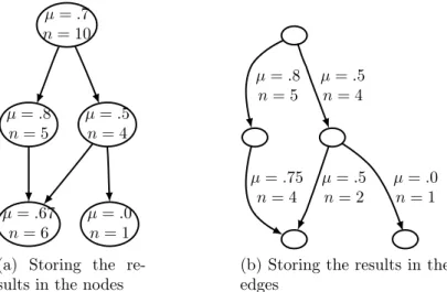
Figure 3 (a) shows a toy game tree where a couple of playouts where performed and the results stored in the nodes. Figure 3 (b) show the same game tree with exactly the same playouts performed, but this time the results were stored on the edges. Almost all the data in Figure 3 (a) can be retrieved in Figure 3 (b). For instance, the data in the middle nodes in Figure 3 (a) is exactly the data in the incoming edges of the middle nodes in Figure 3 (b). Similarly, the data in the bottom left node in Figure 3 (a) can be reconstituted in Figure 3 (b) by aggregating the data on the two incomming edges of the bottom left node; indeed 6 = 4 + 2 and 0.67 = 4×0.75+2×0.54+2 .
1As an implementation note, it is possible to store the aggregations of the edges in the
µ = .0 n = 1 µ = .5 n = 4 µ = .8 n = 5 µ = .67 n = 6 µ = .7 n = 10
(a) Storing the re-sults in the nodes
µ = .5 n = 2 µ = .0 n = 1 µ = .75 n = 4 µ = .8 n = 5 µ = .5 n = 4
(b) Storing the results in the edges
Figure 3: Example of the update-descent backpropagation results stored on nodes and on edges for a toy tree.
3.2. Backpropagation
After the tree was descended and a simulation lead to a payoff, informa-tion has to be propagated upwards. When the game tree is a plain tree, the propagation is straightforward. The traversed nodes are exactly the ancestors of the leaf node from which the simulation was performed. The edges to be updated are thus easily accessed and for each edge, one simulation is added to the counter and the total score is updated. Similarly, in the hash-table solution, the traversed edges are stored on a stack and they are updated the same way.
In the general DAG problem however, many distinct algorithms are pos-sible. The ancestor edges are a superset of the traversed edges and it is not clear which need to be updated and if and how the aggregation should be adapted. We will be interested in three possible ways to deal with the update step: updating every ancestor edge, updating the descent path, updating the ancestor edges but modifying the aggregation of the edge not belonging to the descent path.
Updating every ancestor edge without modifying the aggregation is simple enough, provided one takes care that each edge is not updated more than once after each playout. We call this method update-all. Update-all might suffer from deficiencies in schemata like the counter-example presented in Figure 1. The problem in update-all made obvious by this counter-example is that the distribution of playouts in the different available branches does not
correspond to a distribution as given by UCT: assumption 3 is not satisfied. The other straightforward method is to update only the traversed edges, we call it update-descent. This method is very similar to the standard UCT algorithm implemented on a regular tree and it is used in the simple way. When such a backpropagation is selected, the selection mechanism can be adjusted so that transpositions are taken into account when evaluating a move. The possibilities for the selection mechanism are presented in the following section.
The backpropagation procedure advocated in [10] for their selection pro-cedure UCT3 is also noteworthy. The same behaviour could be obtained directly with the update-descent backpropagation (Section 3.3), but it is fast and can be generalised to our framework (Section 3.4)
3.3. Selection
The descent of the game tree can be described as follows. Start from the root node. When in a node a, select a move m available in a using a selection procedure. If m corresponds to an edge in the game tree, move along that edge to another node of the tree and repeat. If m does not correspond to an edge in the tree, consider the position b resulting from playing m in a. It is possible that b was already encountered and there is a node representing b in the tree, in this case, we have just discovered a transposition, build an edge from a to b, move along that edge and repeat the procedure from b. Otherwise construct a new node corresponding to b and create an edge between a and b, the descent is finished.
The selection process consists in selecting a move that maximises a given formula. State of the art implementations usually rely on complex formulae that embed heuristics or domain specific knowledge, but the baseline remains the UCT formula defined in equation 2.2
When the game tree is a DAG and we use the update-descent backpropa-gation method, the equation 1 does not hold anymore, so it is not absurd to look for another way of estimating the value of a move than the UCT value. Simply put, equation 1 says that all the needed information is available lo-cally, however deep transpositions can provide useful information that would not be accessible locally.
For instance in the partial game tree in Figure 2, it is desirable to use the
information provided by the transpositions in node b and c in order to make the right choice at node a. The local information in a is not enough to decide confidently between b and c, but if we have a look at the outgoing edges of b and c then we will have more information. This example could be adapted so that we would need to look arbitrarily deep to get enough information.
We define a parametric adapted score to try to take advantage of the transpositions to gain further insight in the intrinsic value of the move. The adapted score is parameterized by a depth d and is written for an edge e µd(e). µd(e) uses the number of playouts, the mean payoff and the adapted
score of the descendants up to depth d. The adapted score is given by the following recursive formula.
µ0(e) = µ(e) (4) µd(e) = P f ∈c(e)µd−1(f ) × n(f ) P f ∈c(e)n(f ) (5)
The UCT algorithm uses an exploration factor to balance concentration on promising moves and exploration of less known paths. The exploration factor of an edge tries to quantify the information directly available at it. It does not allow to acknowledge that transpositions occurring after the edge offer additional information to evaluate the quality of a move. So just as we did above with the adapted score, we define a parametric adapted exploration factor to replace the exploration factor. Specifically, for an edge e, we define a parametric move exploration that accounts for the adaptation of the number of payoffs available at edge e and is written nd(e) and a parametric origin
exploration that accounts for the adaptation of the total number of payoffs at the origin of e and is written pd(e). The parameter d also refers to a depth.
nd(e) and pd(e) are defined by the following formulae.
n0(e) = n(e) (6) nd(e) = X f ∈c(e) nd−1(f ) (7) pd(e) = X f ∈b(e) nd(f ) (8)
In the MCTS algorithm, the tree is built progressively as the simulations are run. So any aggregation of edges built after edge e will lack the infor-mation available in µ0(e) and n0(e). This can lead to a leak of information
that becomes more serious as the depth d grows. If we attach µ0(e) and n0(e) along µ(e) and n(e) to an edge it is possible to avoid the leak of information and to slightly adapt the above formulae to also take advantage of this in-formation. Another advantage of the following formulation is that is avoids to treat separately edges without any child.
µ0(e) = µ(e) (9) µd(e) = µ0(e) × n0(e) +P f ∈c(e)µd−1(f ) × n(f ) n0(e) +P f ∈c(e)n(f ) (10) n0(e) = n(e) (11) nd(e) = n0(e) + X f ∈c(e) nd−1(f ) (12) pd(e) = X f ∈b(e) nd(f ) (13)
If the height of the partial game tree is bounded by h, then there is no difference between a depth d = h and a depth d = h + x for x ∈ N.3 When
d is chosen sufficiently big, we write d = ∞ to avoid the need to specify any bound. Since the underlying graph of the game tree is acyclic, if h is a bound on the height of an edge e then h − 1 is a bound on the height of any child of e, therefore we can write the following equality which recalls equation 1.
µ∞(e) = µ0(e) × n0(e) +P f ∈c(e)µ∞(f ) × n(f ) n0(e) +P f ∈c(e)n(f ) (14)
The formulae proposed do not ensure that any playout will not account for more than once in the values of nd(e) and pd(e). However a playout
can only be counted multiple times if there are transpositions in the subtree starting after e. It is not clear to the authors how a transposition in the subtree of e should affect the confidence in the adapted score of e. Thus, it is not clear whether such playouts need to be accounted several times or just once. Admitting several accounts gives rise to a simpler formula and was chosen for this reason.
3For instance, if the game cannot last more thanh moves or if one node is created after
each playout and there will not be more thanh playouts, then the height of the game tree is bounded byh.
We can now adapt formula 2 to use the adapted score and the adapted exploration to give a value to a move. We define the adapted value of an edge e with parameters (d1, d2, d3) ∈ N3 and exploration constant c to be
ud1,d2,d3(e) = µd1(e) + c ×
qlog p
d2(e)
nd3(e) . The notation (d1, d2, d3) makes it easy
to express a few remarks about the framework.
• When no transpositions occur in the game, such as when the board state includes the move list, every parametrisation gives rise to exactly the same selection behaviour which is also that of the plain UCT algorithm. • The parametrisation (0, 0, 0) is not the same as completely ignoring transpositions since each position in the game appears only once in the game tree when we use parametrisation (0, 0, 0).
• The simple way (see Section 2) can be obtained through the (1, 0, 1) parametrisation.
• The selection rules in [10] can be obtained through our formalism: UCT1 corresponds to parametrisation (0, 0, 0), UCT2 is (1, 0, 0) and UCT3 is (∞, 0, 0).
• It is possible to adapt the UCT value in almost the same way when the results are stored in the nodes rather than in the edges but it would not be possible to have a parametrisation similar to any of d1, d2 or d3
equal to zero.
3.4. Efficient selection through incremental backpropagation
The definitions of µd1, pd2, and nd3 can be naturally transformed into
recursive algorithms to compute the adapted value of an edge. In MCTS implementations, the descent part usually constitute a speed bottleneck. It is therefore a concern that using the plain recursive algorithm to compute the adapted mean could induce a high performance cost. Moreover, most of the values will not change from one iteration to the next and so they can be memoized.
To accelerate the descent procedure, we store in each edge e the current values for µd1(e), nd2(e), and nd3(e) as long as n0(e). nd2 allows to compute
easily pd2 and is easier to update. Then we suggest a generalisation of the
backpropagation rule used for the UCT3 selection procedure [10] that we call updated1,d2,d3.
Consider the leaf node l from which the playout was performed. We call ad(x) the set of the ancestors of x at distance at most d from x. For instance,
a0(x) = {x}, a1(x) = {y|x ∈ c(y)} ∪ {x} is the set of the parents of x plus
x. Notice that for each edge e not situated on the traversed path and not belonging to ad1(l), the adapted mean value is not altered by the playout.
Similarly, if e /∈ ad2(l) then nd2(e) is not altered.
Updating the nd2 (resp. nd3) value of the relevant nodes is
straightfor-ward. We simply need to add one to the nd2 (resp. nd3) value of each edge
on the traversed path and each edge in ad2(l) (resp. ad3(l)).
Updating the µd1 value is a bit more involved. We call ∆µd1(e) the
variation of µd1(e) induced by the playout. If e is not in ad1(l) nor in the
traversed path, then ∆µd1(e) = 0. ∆µd1(l) can be directly computed from
the payoff of the playout and the values stored at l. For each other edge e, we use the formula:
∆µ(e) = P f ∈c(e)∆µ(f ) × n(f ) n0(e) +P f ∈c(e)n(f ) (15) 4. Experimental results
In the following experimental results, transpositions were detected by structural comparison of the positions. We used a hash-table where each key k was associated to a list l of pair (position, data). The list l contains the list of every position encountered having key k. To look for a position in the table, we first compute a hash-key for it and then look for the exact position in the corresponding association list. This technique allows for a relatively high speed of execution provided there are few hash collisions. It is also lossless in that it allows a perfect distinction between every position. On the other hand, this method makes it necessary to store one position for each node in the tree which is very memory consumming. Given that we never had more than 100,000 nodes in a memory in these experiments, lack of memory was not a bottleneck and this method was acceptable for our purpose.
4.1. Tests on leftright
leftright is an artificial one player game already used in [13] under the name “left move”, at each step the player is asked to chose to move Left or to move Right; after a given number of steps the score of the player is
75 80 85 90 95 100 0 1 2 3 4 5 6 7 S co re d3 µ0 µ2 µ5 µ∞
Figure 4: leftright results.
the number of steps walked towards Left. A position is uniquely determined by the number of steps made towards Left and the total number of moves played so far, transitions are therefore very frequent. If there are h steps, the full game tree has only h×(h−1)2 nodes when transpositions are recognised. Otherwise, the full game tree has 2h nodes.
We used 300 moves long games for our tests. Each test was run 200 times and the standard error is never over 0.3% on the following scores.
The UCT algorithm performs well at leftright so the number of sim-ulations had to be low enough to get any differentiating result. We decided to run 100 playouts per move. The plain UCT algorithm without detection of transpositions with an exploration constant of 0.3 performs 81.5%, that is in average 243.5 moves out of 300 were Left. We also tested the update-all backpropagation algorithm which scored 77.7%. We tested different values for all three parameters but the scores almost did not evolve with d2 so for
the sake of clarity we present results with d2 set to 0 in Figure 4.
The best score was 99.8% with the parametrisation (∞, 0, 1) which basi-cally means that in average less than one move was played to the Right in each game. Setting d3 to 1 generally constituted a huge improvement.
Rais-ing d1 was consistently improving the score obtained, eventually culminating
4.2. Tests on Hex
hex is a two-player zero sum game that cannot end in a draw. Every game will end after at most a certain number of moves and can be labelled as a win for Black or as a win for White. Rules and details about hex can be found in [14]. Various board sizes are possible, sizes from 1 to 8 have been computer solved [15]. Transpositions happen frequently in hex because a position is completely defined by the sets of moves each player played, the particular order that occurred before has no influence on the position. MCTS is quite successful in Hex [6], hence Hex can serve as a good experimentation ground to test our parametric algorithms.
hex offers a strong advantage to the first player and it is common practice to balance a game with a compulsory mediocre first move.4 We used a size 5
board with an initial stone on b2. Each test was a 400 games match between the parametrisation to be tested and a standard Artificial Intelligence (A.I.) In each test, the standard A.I. played Black on 200 games and White on the remaining 200 games. The reported score designates the average number of games won by a parametrisation. The standard error was never over 2.5%.
The standard A.I. used the plain UCT algorithm with an exploration constant of 0.3, it did not detect transpositions and it could perform 1000 playouts at each move. We also ran a similar 400 games match between the standard A.I. and an implementation of the update-all backpropagation algo-rithm with an exploration constant of 0.3 and 1000 playouts per move. The update-all algorithm scored 51.5% which means that it won 206 games out of 400. The parametrisation to be tested also used a 0.3 exploration constant and 1000 playouts at each move. The results are presented in Figure 5 for d2
set to 0 and in Figure 6 for d2 set to 1.
The best score was 63.5% with the parametrisation (0, 1, 2). It seems that setting d1 as low as possible might improve the results, indeed with d1 = 0
the scores were consistently over 53% while having d1 = 1 led to having scores
between 48% and 62%. Setting d1 = 0 is only possible when the payoffs are
stored per edge instead of per node as discussed in Section 3.1.
One can contrast the fact that the optimal value for d1 in a one player
game was ∞ and that it is 0 in the two-player game hex. One possible explanation for this behaviour would be that the higher d1 is, the more
information is taken into account, however in a two-player game, alternating
40 42 44 46 48 50 52 54 56 58 60 62 0 1 2 3 4 5 S co re d3 µ0 µ1 µ2 µ4
Figure 5: hex results with d2set to 0
40 45 50 55 60 65 0 1 2 3 4 5 S co re d3 µ0 µ1 µ2 µ4
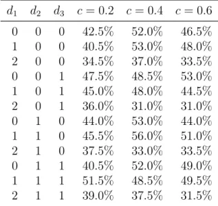
Table 1: Results of various configurations of UCD against UCT without transposition table at6 × 6 go d1 d2 d3 c = 0.2 c = 0.4 c = 0.6 0 0 0 42.5% 52.0% 46.5% 1 0 0 40.5% 53.0% 48.0% 2 0 0 34.5% 37.0% 33.5% 0 0 1 47.5% 48.5% 53.0% 1 0 1 45.0% 48.0% 44.5% 2 0 1 36.0% 31.0% 31.0% 0 1 0 44.0% 53.0% 44.0% 1 1 0 45.5% 56.0% 51.0% 2 1 0 37.5% 33.0% 33.5% 0 1 1 40.5% 52.0% 49.0% 1 1 1 51.5% 48.5% 49.5% 2 1 1 39.0% 37.5% 31.5%
turns introduces a bias leading to poor performance.
4.3. Tests on go
In order to test Upper Confidence bound for Direct acyclic graph (UCD) in another game we choose to make it play go. Size 9 × 9 and 19 × 19 are standard for go, but given the size of the parameter space and the large number of playouts per move needed so that many transpositions occur on bigger boards, we decided to run the experiments on size 6 × 6. The number of playouts is fixed to 10000 in order to have enough transpositions to detect a difference in strength. Each test consists in playing 200 games against UCT without transposition table.
Table 1 gives the results for various configurations of UCD against UCT without transposition table. The game is 6 × 6 go with a komi of 5.5. UCT without transposition table uses the best found constant c = 0.4. A first interesting result in this table is that the usual configuration of UCT with transposition table (d1 = 1, d2 = 0, d3 = 1) only wins 48% of its game
against UCT without transposition table. Another interesting result is that UCD with d1 = 1, d2 = 1 and d3 = 0 wins 56% of its games against UCT
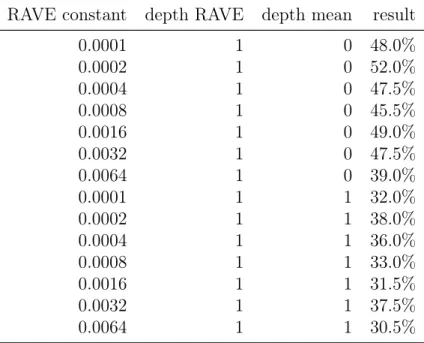
Table 2: Results of various configurations of RAVE UCD against standard RAVE at6 × 6 go
RAVE constant depth RAVE depth mean result
0.0001 1 0 48.0% 0.0002 1 0 52.0% 0.0004 1 0 47.5% 0.0008 1 0 45.5% 0.0016 1 0 49.0% 0.0032 1 0 47.5% 0.0064 1 0 39.0% 0.0001 1 1 32.0% 0.0002 1 1 38.0% 0.0004 1 1 36.0% 0.0008 1 1 33.0% 0.0016 1 1 31.5% 0.0032 1 1 37.5% 0.0064 1 1 30.5%
Another possibility for UCD is to adapt the idea to the Rapid Action Value Estimation (RAVE) heuristic [16]. In this case instead of using the All Moves as First (AMAF) values of the node, the program mixes the AMAF values of all its children. This way it also uses the playouts of its children that come from another node to compute the AMAF value.
Table 2 gives the results for various configurations of RAVE UCD against standard RAVE. We can observe that RAVE UCD is often worse than stan-dard RAVE.
4.4. Tests on General Game Playing
Game program usually embed a important body of knowledge that is specific of the game they play. This knowledge is used by the designer be-forehand and limit somewhat the generality of the program. While a program like Deep Blue is able to play well chess, it can not play a match of check-ers, or even tictactoe: while an expert in its domain, the playing program is limited to one game in its abilities, and these are not easily extended to other domains or even to other games.
The Logic Group at the university of Stanford addresses this limitation with GGP. In a GGP match, the players receive the rules of the game they have to play in a specific language called Game Description Language from a Game Master. The players have a set time, usually between 30 seconds and 20 minutes, to analyse the game. After that analyse phase, every player repeatedly selects a move in a fixed time, usually between 10 seconds and 1 minute, and sends it to the Game Master that combines them in a joint move transmitted back to all the players.
The Logic Group organise an annual competition at the summer con-ference of the Association for the Advancement of Artificial Intelligence (AAAI) [17].
As they do not know beforehand the games that will be played, General Game Player have to analyse the rules of the game to select a method that work well for the game at hand, or use only methods that work well for all the conceivable games. Ary, our General Game Playing program uses UCT to play general games. It won the 2009 and the 2010 GGP competitions.
Due to the interpretation of the game descriptions in GDL, current general game players are only able to perform a very limited number of playouts in the given reflexion time.
The tests consist in having a parameterized version of Ary playing games against Ary without transposition detection. Parameters for the depth of the calculation for the mean, the parent playouts and the child playouts were tested with values 0, 1 and 2. Games have been played with 10 seconds per move. The UCT constant c was fixed to 40 as games results vary between 0 and 100. Both players ran on the same machine, from a pool of 35 computers, each with 2 GB of memory and dual core processors of frequencies between 2 and 2.5 GHz.
We tested using the games breakthrough, knightthrough, pawn whopping, capture the king, crisscross, connect 4, merrills, othello, pentago, and quarto.
breakthrough is played on a chess board; each player has two rows of pawns, moving forward or diagonally and try to have one pawn breaking through adversary line to attain the opposite row of the board. knigth-through has the same structure, but all the pieces move forward like knights in chess. pawn whopping is a variant where the players have only pawns, disposed at the beginning and moving as in ordinary chess. capture the king is a simplified variation of chess where the goal is to be the first to capture the opponent king. crisscross is a simplified version of chinese
checkers where the players must move their four pieces on the other side of a two cells wide cross inscribed in 6 square board. connect 4, merrills, othello, pentago and quarto are the usual games. The description of all these games can be found on http://euklid.inf.tu-dresden.de: 8180/ggpserver.
The tables containing the results are given at the end of the paper. We tested the values 0, 1 and 2 for d1, d2, and d3. Each percentage in the table
is the result of at least 200 games.
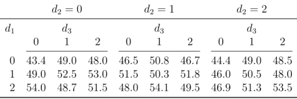
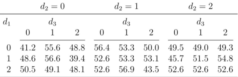
For breakthrough the best combination is (2, 1, 1) which has an average score of 54.1%. For capture the king the best combination is (1, 0, 0) which has an average score of 56.5%. For connect 4 the best combination is (2, 1, 2) which has an average score of 70.9%. According to the table, the transposition table helps a lot at connect 4 since many values in the table are above 60%. The usual way of dealing with transpositions (1, 0, 1) gives 63.9%. For crisscross the best combination is (0, 2, 0) which has an average score of 62.0% whereas the usual combination (1, 0, 1) has an average score of 55.1%. For knightthrough the best combination is (2, 1, 1) which has an average score of 56.9% which is very close to the score of 56.6% of the usual combination. For merrills the best combination is (1, 2, 2) with a score of 55.8% which is better than the 48.9% of the usual combination. For othello the best combination is (1, 1, 1) with a score of 59.2% which is better than the 46.5% of the usual combination. For pawn whopping the best combination is again (1, 1, 1) with a score of 59.8% which is better than the 50.5% of the usual combination. For pentago the best combination is (0, 2, 1) with a score of 56.8% which is close to the 53.8% of the usual combination. For quarto the best combination is (0, 0, 0) with a score of 55.8% which is better than the 50.7% of the usual combination.
In all these games the best combination is different from the usual com-bination. In some games the results are quite close to the results without transposition table. However in some games such as connect 4 for exam-ple, the transposition table helps a lot and the best combination gives much better results than the usual combination.
5. Conclusion and Future Work
We have presented a parametric algorithm to deal with transpositions in MCTS. Different parameters did improve on usual MCTS algorithms for games such as leftright, hex or connect 4.
Table 3: Results for the game of Breakthrough d2 = 0 d2 = 1 d2 = 2 d1 d3 d3 d3 0 1 2 0 1 2 0 1 2 0 43.4 49.0 48.0 46.5 50.8 46.7 44.4 49.0 48.5 1 49.0 52.5 53.0 51.5 50.3 51.8 46.0 50.5 48.0 2 54.0 48.7 51.5 48.0 54.1 49.5 46.9 51.3 53.5
In this paper we did not deal with the graph history interaction prob-lem [18]. In some games the probprob-lem occurs and we might adapt the MCTS algorithm to deal with it.
We have defined a parameterized value for moves that integrates the in-formation provided by some relevant transpositions. The distributions of the values for the available moves at some nodes do not necessarily correspond to a UCT distribution. An interesting continuation of our work would be to de-fine an alternative parametric adapted score so that the arising distributions would still correspond to UCT distributions.
Another possibility to take into account the information provided by the transpositions is to treat them as contextual side information. This informa-tion can be integrated in the value using the RAVE formula [16], or to use the episode context framework described in [19].
Acknowledgements
We would like to thank the anonymous reviewers for their comments that helped improve this article.
Table 4: Results for the game of Capture the king d2 = 0 d2 = 1 d2 = 2 d1 d3 d3 d3 0 1 2 0 1 2 0 1 2 0 54.1 49.6 49.2 46.3 46.3 47.6 52.4 47.7 49.4 1 56.5 50.0 44.9 48.8 51.4 49.4 49.2 50.2 56.1 2 42.3 46.1 48.4 51.4 48.2 47.6 44.9 50.8 47.8
Table 5: Results for the game of Connect4
d2 = 0 d2 = 1 d2 = 2 d1 d3 d3 d3 0 1 2 0 1 2 0 1 2 0 52.2 46.1 58.3 66.7 48.9 42.8 58.9 52.8 52.8 1 69.4 63.9 50.6 61.7 67.8 53.3 66.1 60.6 54.4 2 57.2 56.7 67.8 61.1 58.3 70.9 57.2 62.2 70.7
Table 6: Results for the game of Crisscross
d2 = 0 d2 = 1 d2 = 2 d1 d3 d3 d3 0 1 2 0 1 2 0 1 2 0 58.0 52.2 43.1 61.1 51.4 45.8 62.0 50.8 43.5 1 56.5 55.1 49.6 57.4 58.8 55.0 57.4 56.9 50.0 2 59.7 54.6 58.8 57.9 56.9 59.2 57.9 58.9 56.9
Table 7: Results for the game of Knightthrough d2 = 0 d2 = 1 d2 = 2 d1 d3 d3 d3 0 1 2 0 1 2 0 1 2 0 41.2 55.6 48.8 56.4 53.3 50.0 49.5 49.0 49.3 1 48.6 56.6 39.4 52.6 53.3 53.1 45.7 51.5 54.8 2 50.5 49.1 48.1 52.6 56.9 43.5 52.6 52.6 52.6
Table 8: Results for the game of Merrills
d2 = 0 d2 = 1 d2 = 2 d1 d3 d3 d3 0 1 2 0 1 2 0 1 2 0 49.0 52.6 50.8 50.6 47.8 50.0 47.9 54.2 50.4 1 55.7 48.9 50.2 46.4 50.0 52.5 47.0 48.3 55.8 2 47.8 52.0 52.5 50.8 52.2 54.8 47.7 47.5 51.7
Table 9: Results for the game of Othello-comp2007
d2 = 0 d2 = 1 d2 = 2 d1 d3 d3 d3 0 1 2 0 1 2 0 1 2 0 54.1 50.0 52.9 49.3 46.1 46.4 45.7 50.2 51.1 1 42.1 46.5 42.6 46.9 59.2 50.6 53.4 47.6 51.4 2 44.2 52.9 46.4 54.1 47.0 51.6 43.8 49.8 53.2
Table 10: Results for the game of Pawn whopping d2 = 0 d2 = 1 d2 = 2 d1 d3 d3 d3 0 1 2 0 1 2 0 1 2 0 48.0 53.7 51.0 51.2 52.1 50.6 53.8 48.2 49.8 1 52.0 50.5 50.8 50.8 59.8 52.6 42.8 57.4 51.9 2 50.0 49.0 49.1 46.8 52.1 52.8 47.5 49.0 58.6
Table 11: Results for the game of Pentago 2008
d2 = 0 d2 = 1 d2 = 2 d1 d3 d3 d3 0 1 2 0 1 2 0 1 2 0 55.8 53.4 56.0 55.3 51.5 45.5 52.8 56.8 46.2 1 46.6 53.8 47.2 51.0 50.0 49.8 51.7 53.8 48.3 2 49.6 52.1 52.4 48.3 52.6 53.0 48.9 53.3 53.5
Table 12: Results for the game of Quarto
d2 = 0 d2 = 1 d2 = 2 d1 d3 d3 d3 0 1 2 0 1 2 0 1 2 0 55.8 47.4 49.5 53.7 47.5 49.8 51.2 51.9 47.9 1 50.2 50.7 50.2 49.1 52.1 49.8 48.6 48.9 48.6 2 50.9 51.4 50.4 51.1 49.6 46.2 51.2 47.6 50.2
References
[1] R. Coulom, Efficient selectivity and back-up operators in monte-carlo tree search, in: Proceedings of the 5th Conference on Computers and Games (CG’2006), Vol. 4630 of LNCS, Springer, Torino, Italy, 2006, pp. 72–83.
[2] R. Coulom, Computing Elo ratings of move patterns in the game of Go, ICGA Journal 30 (4) (2007) 198–208.
[3] S. Gelly, D. Silver, Achieving master level play in 9 x 9 computer go, in: Proceedings of the 23rd national conference on Artifical Intelligence (AAAI’08), 2008, pp. 1537–1540.
[4] C.-S. Lee, M. Müller, O. Teytaud, Special issue on monte carlo tech-niques and computer go, IEEE Transactions on Computational Intelli-gence and AI in Games 2 (4) (2010) 225–228.
[5] A. Rimmel, O. Teytaud, C.-S. Lee, S.-J. Yen, M.-H. Wang, S.-R. Tsai, Current frontiers in computer go, IEEE Transactions on Computational Intelligence and AI in Games 2 (4) (2010) 229–238.
[6] T. Cazenave, A. Saffidine, Utilisation de la recherche arborescente Monte-Carlo au Hex, Revue d’Intelligence Artificielle 23 (2-3) (2009) 183–202.
[7] B. Arneson, R. B. Hayward, P. Henderson, Monte carlo tree search in hex, IEEE Transactions on Computational Intelligence and AI in Games 2 (4) (2010) 251–258.
[8] M. H. M. Winands, Y. Björnsson, J.-T. Saito, Monte carlo tree search in lines of action, IEEE Transactions on Computational Intelligence and AI in Games 2 (4) (2010) 239–250.
[9] D. M. Breuker, Memory versus search in games, Phd thesis, Universiteit Maastricht (1998).
[10] B. E. Childs, J. H. Brodeur, L. Kocsis, Transpositions and move groups in Monte Carlo Tree Search, in: Proceedings of the IEEE Symposium on Computational Intelligence and Games (CIG’08), 2008, pp. 389–395.
[11] J. Méhat, T. Cazenave, Combining UCT and nested Monte-Carlo search for single-player general game playing, IEEE Transactions on Compu-tational Intelligence and AI in Games 2 (4) (2010) 271–277.
[12] L. Kocsis, C. Szepesvàri, Bandit based monte-carlo planning, in: Proceedings of the 17th European Conference on Machine Learning (ECML’06), Vol. 4212 of LNCS, Springer, 2006, pp. 282–293.
[13] T. Cazenave, Nested monte-carlo search, in: Proceedings of the 21st In-ternational Joint Conference on Artificial Intelligence (IJCAI-09), 2009, pp. 456–461.
[14] C. Browne, Hex Strategy: Making the Right Connections, Natick, MA, 2000.
[15] P. Henderson, B. Arneson, R. B. Hayward, Solving 8x8 Hex, in: C. Boutilier (Ed.), Proceedings of the 21st International Joint Confer-ence on Artificial IntelligConfer-ence (IJCAI-09), 2009, pp. 505–510.
[16] S. Gelly, D. Silver, Combining online and offline knowledge in UCT, in: Proceedings of the 24th International Conference on Machine Learning (ICML’07), 2007, pp. 273–280.
[17] M. Genesereth, N. Love, General game playing: Overview of the AAAI competition, AI Magazine 26 (2005) 62–72.
[18] A. Kishimoto, M. Müller, A general solution to the graph history in-teraction problem, in: Proceedings of the 19th national conference on Artifical Intelligence (AAAI’04), San Jose, California, 2004, pp. 644–649. [19] C. D. Rosin, Multi-armed bandits with episode context, in: Proceedings of the International Symposium on Artificial Intelligence and Mathe-matics (ISAIM’10), Fort Lauderdale, Florida, 2010.