HAL Id: hal-02545925
https://hal.archives-ouvertes.fr/hal-02545925
Submitted on 17 Apr 2020HAL is a multi-disciplinary open access
archive for the deposit and dissemination of sci-entific research documents, whether they are pub-lished or not. The documents may come from teaching and research institutions in France or abroad, or from public or private research centers.
L’archive ouverte pluridisciplinaire HAL, est destinée au dépôt et à la diffusion de documents scientifiques de niveau recherche, publiés ou non, émanant des établissements d’enseignement et de recherche français ou étrangers, des laboratoires publics ou privés.
inversion of field and seismic data
Laurent Moretti, A. Mangeney, F. Walter, Yann Capdeville, T. Bodin, E.
Stutzmann, A Le friant
To cite this version:
Laurent Moretti, A. Mangeney, F. Walter, Yann Capdeville, T. Bodin, et al.. Constraining landslide characteristics with Bayesian inversion of field and seismic data. Geophysical Journal International, Oxford University Press (OUP), 2020, 221 (2), pp.1341-1348. �10.1093/gji/ggaa056�. �hal-02545925�
Constraining landslide characteristics with Bayesian
inversion of field and seismic data
L. Moretti1,2,A. Mangeney1,2,3, F. Walter4, Y. Capdeville5, T. Bodin6, E. Stutzmann1, A. Le Friant1
1Institut de Physique du Globe de Paris - UMR 7154, PRES Sorbonne Paris Cité, Paris, France
2Université de Paris, Paris, France
3INRIA-J. L. Lions, France
4ETH Zurich, Switzerland
5Laboratoire de Planétologie et Géodynamique de Nantes, Nantes, France
6Univ Lyon, ENS de Lyon, CNRS, UMR 5276 LGL-TPE, F-69622, Villeurbanne, France
20 August 2019
SUMMARY
Using a fully non-linear Bayesian approach and a granular flow model we invert for land-slide parameters (volume, release geometry, and rheology) from different kinds of obser-vations. Synthetic tests show that the runout distance and the deposit area by themselves do not constrain landslide parameters. In contrast, the thickness distribution of landslide deposits provides better constraints on landslide parameters. The same is true for the force history applied by the landslide to the ground and which contains information on the landslide dynamics. Therefore, inverting force histories calculated from seismic broad-band records is an important alternative to inverting thickness distributions of landslide deposits, which are usually difficult to obtain. We test the method on the 1997 Boxing Day debris avalanche on Montserrat Island, which involved 40 − 50 Mm3. The Bayesian inversion and granular flow model provide good estimates for volume, release geome-try and effective friction coefficient. This study thus underlines the value of broadband
seismic records as observations to monitor landslides and validate their numerical flow models.
1 INTRODUCTION
Landslides and avalanches are key erosion processes and represent major natural hazards. Despite important research efforts, the mechanisms that govern flow dynamics and deposition in a natural environment are still unclear. Key questions remain unanswered, such as the origin of the high mobility of some natural flows (e.g., Legros, 2002; Iverson et al., 2011; Lucas et al., 2014).
Numerical granular flow models are an important tool to investigate landslides and avalanches (Delannay et al., 2017). However, poor availability of field measurements of flow dynamics makes it difficult to validate these models. Therefore, a common “inverse approach” is to fit model output to observed landslide characteristics like volume and shape of the released mass, deposit area and runout distance to constrain effective friction, a key underlying rheological parameter (Lucas et al., 2011; Kelfoun, 2005; Pirulli et al., 2015).
A problem with the inverse approach is that the thickness distributions of landslide deposits are rarely available as they require Digital Elevation Models (DEM’s) immediately before and after the event. Unfortunately, landslide deposits are generally modified by secondary flows or post-event ero-sion and for landslides terminating in water bodies, deposition DEM’s may be nearly impossible to come by. Furthermore, during the stopping phase of granular flows, local surface rearrangements mod-ify the final shape of the deposit, as shown in laboratory experiments (e.g., Farin et al., 2014). This rearrangement is difficult to take into account in landslide models. As a result, observed deposits may incorrectly constrain landslide dynamics and rheology. Another key issue is that landslide models may well reproduce the deposit even though the simulated dynamics are not correct (e.g., Mangeney-Castelnau et al., 2005; Ionescu et al., 2015). Therefore, more easily obtainable observations, such as deposit area and runout distance may not be appropriate either.
A range of studies suggests that long-period seismic signals reflecting the history of the force exerted by the landslide mass movement onto the ground may be a better constraint of landslide dy-namics (e.g., Kanamori et al., 1984; Kawakatsu, 1989; Brodsky et al., 2003; Favreau et al., 2010; Lin et al., 2010; Moretti et al., 2012; Allstadt et al., 2013; Ekström and Stark, 2013; Yamada et al., 2018)). In contrast to static observations of before/after landscapes, comparing this seismically observed force history with the force simulated by landslide models provides a diagnostic of landslide dynamics. In this way, seismic records can constrain the landslide volume, the number of sub-events, the effect of unusual ground properties, such as glacier ice and erosion processes (Favreau et al., 2010; Moretti et
al., 2012, 2015). Given this perspective, two questions have to be answered: First, how does the inver-sion of seismically-derived force history compare with the inverinver-sion of deposit data (runout distance, area of the deposit, spatial distribution of the thickness of the deposit)? Second, what level of con-straint can be achieved on landslide parameters (volume, shape of the landslide mass before release, effective friction coefficient, etc.) from inversion of seismic data?
To address these questions we use a Bayesian inversion of synthetic and real data to constrain landslide parameters (volume, 3D shape of the released mass, effective friction coefficient). We show that runout distance or the deposit area alone cannot constrain these parameters, whereas the force history obtained from seismic data strongly constrains the landslides parameters, nearly as well as the spatial distribution of deposit thickness. Our study thus demonstrates that seismic measurements, which are easy to obtain compared to accurate deposition DEMS’s, offer a valuable monitoring tool and important insights into landslide dynamics.
2 BAYESIAN INVERSION
We formulate our inversion for landslide parameters in a Bayesian framework (e.g., Sivia and Skilling, 2006) where the solution is the expression for the posterior probability density function (PDF) p(m|d) of our landslide model parameters m conditioned on observed data d:
p(m|d) = p(d|m) × p(m)
p(d) (1)
p(d) is the prior PDF reflecting any knowledge about landslide parameters independent of our observations d and p(d|m) is the likelihood function, i.e. the probability of making observations d conditioned by a model m. The PDF of observations p(d) (sometimes referred to as “evidence”) does not depend on model parameters m and can be determined via normalization of the posterior PDF.
To sample the posterior PDF in Equation (1), we employ the Markov-Chain-Monte-Carlo (MCMC) algorithm (Sambridge and Mosegaard, 2002; Gallagher et al., 2009). We approximate the likelihood function by a multivariate Gaussian PDF:
p(d|m) = 1 (2π)1/2|V|N/2e −1 2((d−g(m)) tV−1(d−g(m))) (2)
where V is the covariance matrix of data errors, g(m) is the forward model prediction for the parameter set m and N is the number of data points. At each iteration the MCMC algorithm randomly chooses a new model parameter set m0as a perturbation of the current parameter set m and calculates an acceptance probability α = min(1, p(d|m0)/p(d|m)). The proposed model m0 is accepted with
probability α. If α = 1 (m0 gives an equal or higher probability than m), m0is accepted and becomes the new best parameter set m. Otherwise, a random number u between 0 and 1 is chosen, if u < α, the parameter set m0 is accepted, otherwise it is rejected. The MCMC algorithm is designed to generate an ensemble of parameter sets that are distributed according to the posterior distribution. In this way, the posterior PDF can be approximated by a histogram of all the accepted parameter sets. The more iterations we perform the better the approximation to the true posterior PDF p(m|d) of each parameter.
3 LANDSLIDE MODEL AND PARAMETER SET
To produce model predictions of our landslide parameters, we use the numerical code SHALTOP that simulates landslides over a 3D topography (Bouchut et al., 2003; Bouchut and Westdickenberg, 2004; Mangeney et al., 2007). SHALTOP is a continuum model based on the depth-averaged thin layer approximation and describes granular flows by taking into account a Coulomb type friction law involving an effective friction coefficient µ = tan δ, where δ is the friction angle. Given a parameter set m describing the released mass and the frictional properties, SHALTOP calculates the flow thick-ness h(x, t) (where x is the position vector and t the time), the depth-averaged velocity u(x, t) of the granular media and the force F(t) applied by the landslide to the bed surface (see equation (4) and (5) in Moretti et al., 2015). SHALTOP reliably reproduces laboratory granular flow experiments and real landslides as well as the history of the force inverted from seismic data (Mangeney-Castelnau et al., 2005; Lucas et al., 2011, 2014; Favreau et al., 2010; Hibert et al., 2011; Moretti et al., 2012, 2015; Yamada et al., 2018).
As the main unknowns of the problem, we choose the landslide parameter set m = [δ, h0, l0, w0],
where δ is the friction angle, h0, l0 and w0, are the thickness, length and width of the initial released
mass, respectively (Figure 1a). In the following, 4 independent and separate inversions will be carried out to constrain the landslide parameter set. In each case, different data types will be inverted: (1) the runout distance rf, (2) the area of the deposit Af, (3) the shape of the deposit hf(x), and (4) the force
inverted from seismic data F(t). The goal is to calculate the a posteriori PDF of the parameters and thus to assess which data type best constraint the landslide parameters.
4 INVERSION OF THE CHARACTERISTICS OF A SYNTHETIC GRANULAR FLOW
We first apply the Bayesian approach to synthetic data obtained by simulating a simple granular flow over an inclined plane of inclination angle 10◦. A parabolic-shaped mass of thickness h0 = 30 m,
length l0 = 200 m and width w0= 200 m is released from rest at t = 0 s and spreads down the slope
Table 1. Uncertainties for synthetic landslide parameters.
Parameter Symbol Uncertainty
Runout distance rf 60 m
Deposit area Af 4 ∗ 103m2
Force history F(t) 1.6 ∗ 104kN
Deposit thickness hf(x) 5 m
using SHALTOP with a friction angle δ = 17◦. At each time step the equivalent point source force F(t) is calculated from the spatial integral of the force field F(x, t) applied by the granular mass on the underlying ground.
The simulated force in both the downslope and vertical directions reflects the acceleration and deceleration phases of the landslide (e.g., Brodsky et al., 2003). As a result of the parabolic mass shape, the force in the transverse direction is symmetric over the longitudinal axis through the mass’s center and thus integrates to zero. Consequently, the transverse spreading is poorly constrained by the equivalent point source force F(t). The presence of a more complex topography would provide a non-zero transverse force that would contain information on the transverse spreading dynamics (e.g., Moretti et al., 2015).
We assign a flat PDF to the prior p(m), which means that we do not consider prior information on δ, h0, l0, and w0 other than their possible ranges shown in Figure 1(d-g). We furthermore assume
a diagonal covariance matrix for data errors, which means that the multiple data points of the deposit distribution and force history are not correlated. The assumed measurement uncertainties are typical values for deposit and runout mapping, digital elevation models and inverted forces (Table 1).
4.1 Inversion from deposits data
First, we take the runout distance as the data of the Bayesian inversion, i.e. d = rf, and perform
8000 MCMC iterations, after which the algorithm is expected to provide an ensemble of models representing well enough the posterior distribution. Figure 1d shows that the runout distance is unable to constrain the parameter set: the PDF of all parameters are wide and do not exhibit clear maxima. While the poorly defined maxima of the PDF of h0 and l0 roughly correspond to their real values
(vertical dotted lines in Figure 1), the values of w0and of the friction coefficient δ are not recovered
at all.
Using the deposit area as data, i.e. d = Af, does not improve the results (Figure 1e) but results in
worse determination of the initial thickness h0and length l0. Compared to the inversion of the runout
Figure 1. (a) Initial and (b) final shape of the granular mass simulated using SHALTOP and used as synthetic data for the MCMC inversion (the colors indicate the mass thickness from thin (blue) to 40 m thick (red), (c) corresponding simulated force applied to the ground surface in the vertical (red), downslope (green) and transverse (blue) direction. (d-g) Probability functions of the four parameters δ, h0, l0, and w0inverted using
different data: (d) runout distance rf, (e) deposit area Af, (f) deposit shape hf(x), and (g) force F(t). The
vertical axis of the plots represents the number of accepted parameter sets. The actual values of the parameters (i.e. the input parameters used to simulate the synthetic data) are represented with vertical dotted lines on each plot.
affects deposit area, which we use as data Af. The highest number of accepted models are obtained
for friction angles closer to the real value of δ but with a rather flat histogram shape and the PDF maximum does not correspond to δ = 17◦.
deposit, i.e. d = hf(x), strongly constrains the parameters set. The better performance does not come
as a surprise, because the thickness distribution provides more multiple points compared to the single data point of runout and deposit area. All landslide parameters exhibit peaked PDF’s (Figure 1f). These maxima correspond to the real parameter values with an error of less than 3%. Indeed, after 8000 iterations, the inversion gives δ = 17.44◦ ± 1.11◦, h0 = 30.61 m ±4.35 m, l0 = 198.76 m
±14.98 m, w0= 198.12 m ± 18.24 m.
4.2 Inversion from the force applied to the ground
In the next synthetic test, we used the force simulated by the SHALTOP model as data, i.e. d = F(t) (Figure 1c). This force is obtained from inversion of seismic data (see next section) and is usually more easily available than deposit DEM’s. To be more realistic, we added random noise with amplitudes up to the expected uncertainty (Table 1), still performing 8000 iterations. Figure 1g shows that three parameters are well constrained: h0, l0and δ. The mass width w0is less well constrained, exhibiting
two maxima. This was expected from the vanishing transverse force as discussed above. Nevertheless, the maxima of all the parameters correspond to their real values with an error calculated from the probability functions smaller than 7%. The inversion gives δ = 17.10± 1.50, h
0 = 28.9 m ±3.6 m,
l0 = 196.0 m ±67.1 m and w0 = 205.4 m ±49.0 m.
These results show that the force history F(t) constitutes an observation time series, which is much easier to obtain than the detailed thickness distribution of the deposit hf(x) but still makes it
possible to constrain the landslide parameters. In real cases, where the topography is irregular, the transverse force no longer vanishes and therefore will provide more information on the transverse mass spreading (e.g., Moretti et al., 2012, 2015).
5 REAL LANDSLIDE CASE: THE 1997 BOXING DAY EVENT, MONTSERRAT
We now apply the Bayesian inversion to the Boxing Day debris avalanche that occurred on Montserrat Island on 26th December 1997. In this event, the southern flank collapse of the Soufriere Hills Volcano (18.11◦N, 66.15◦W) generated a debris avalanche with a volume of 40 − 50 Mm3 (Heinrich et al., 2001; Zhao et al., 2014) (Figure 2). We selected this event because (i) it has a simple dynamic history without substantial erosion, motion over a glacier modifying basal fiction (Favreau et al., 2010) or multiple sub-events, (ii) source area outline and topography before the event are available (Sparks et al., 2002).
For the Boxing Day debris avalanche the three components of F(t) (Figure 2c) were obtained by deconvolving the Green’s functions from the record at SJG broadband seismic station (16.71◦N,
Figure 2. (a) Map of Montserrat island where the gray area represents the deposits of the Boxing Day debris avalanche within the White River Valley. (b) Inset map of Montserrat Island in Caribbean Sea. (c) Force history obtained by waveform inversion of the SJG seismic data (red) and by numerical modelling of the avalanche using the parameters deduced from the Bayesian inversion (green). The gray area represents the 66% confidence interval for the ensemble of parameter sets representing the posterior solution. The forces are filtered in the period range 25-40 s.
Figure 3. (a) Initial and (b) final state of the simulation using h0= 184 m, l0= 785.2 m, w0 = 665.6 m and
δ = 14.2◦. A posteriori density probability of (c) δ, (d) h0, (e) w0and (f) l0.
62.18◦W) located about 448 km away from the Soufriere Hills (Figure 2a) (Zhao et al., 2014). In order to optimize the signal-to-noise ratio, the force was inverted in a rather narrow period range T ∈ [25 − 40] s (for details see Zhao et al., 2014). Given this frequency range and a landslide motion, which is small compared to the source-station distance of 448 km, the inverted force corresponds to the spatial integral F(t) calculated with SHALTOP. Finally, Green’s functions were calculated using normal modes summation with the 1D PREM Earth model (Dziewonski and Anderson, 1981) and it should be noted that Moretti et al. (2015) have previously shown that such one-station inversions provide a sufficient constraint of the landslide force history.
As with the synthetic tests we approximate the initial collapsing mass by parabolic shape, defined by 3 parameters: its height h0, length l0and width w0(Figure 3a). Although this is a simplification for
0 50 100 150 200 12
14 16
time (s) mean friction angle (°)
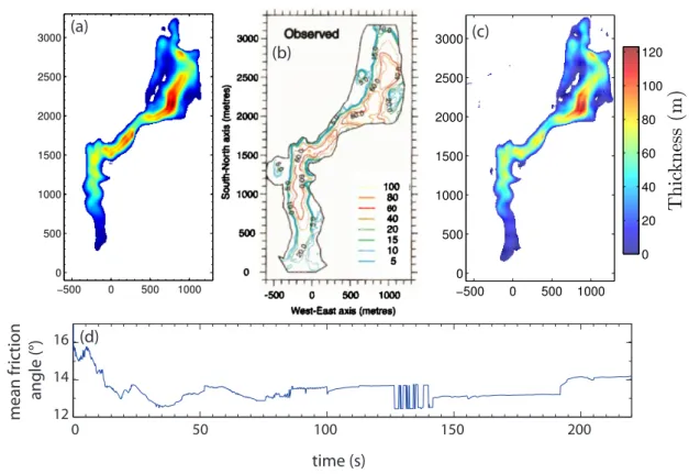
−500 0 500 1000 3000 2500 2000 1500 1000 500 0 T h ic k n es s (m ) 0 20 40 60 80 100 120 (b) (c) (d) −500 0 500 1000 0 500 1000 1500 2000 2500 3000 (a)
Figure 4. Deposits of the Boxing Day avalanche simulated using the parameters h0 = 184 m, l0 = 785.2 m,
w0 = 665.6 m deduced from the Bayesian inversion, with a (a) constant friction coefficient (δ = 14.2◦), (c)
variable friction coefficient (see equation (3), Lucas et al., 2014), and (b) deposit observed on the field extracted from (Heinrich et al., 2001). (d) Friction coefficient as a function of time for the simulation using the friction law (3).
a landslide scar, it allows for an efficient Bayesian inversion and at the same time provides an estimate of volume and surface area covered by the released mass. As previously, we use the force history as data (i.e. d = F(t)) and invert for the landslide parameter set m = [δ, h0, l0, w0] and performed 8000
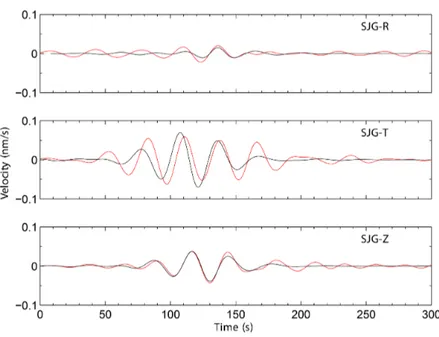
iterations. Note that the seismic signal generated by the force calculated with the best fitting model matches the recorded seismic signal well (Figure 5).
Figure 3(c-f) shows that the shape parameters of the collapsing mass h0, l0 and w0 are well
constrained as the PDF’s exhibit clear maxima. The MCMC algorithm converges toward the values h0 = 184 m ±25.8 m, l0 = 785.2 m ±57.3 m, and w0 = 665.6 m ±52.8 m, leading to a volume
V ∈ [32.7, 58.9] Mm3 with a central value of V = 45.8 Mm3. This is consistent with field observa-tion, which report a volume of 40 − 50 Mm3and a 400 m wide and 400-500 m long source area with a 100 m high head scarp (Sparks et al., 2002; Voight et al., 2002). The slightly larger dimensions from our inversion likely reflect the parabolic approximation of the source geometry.
Figure 5. Ground velocity (i. e. seismic signal) calculated by convolution of the force calculated by the best model (i. e. best parameter set) and the Earth Green’s functions (black lines), and recorded at SJG seismic station (red lines) in the radial, transverse and vertical directions. The signals are filtered between 25 s and 40 s.
well defined solution. Specifically, the PDF exhibits two maxima at δ1 = 14.2◦ ± 0.9◦ and δ2 =
16.6◦ ± 1.4◦ (Figure 3c). Using δ1 underestimates the observed runout distance by only about 150
m while using δ2 leads to an underestimate by about 800 m. The friction angle δ1 = 14.2◦ is close
to the friction angle calibrated by Heinrich et al. (2001) to fit the runout distance when using pre-defined field estimates of the dimensions of the collapsing mass. It is also very close to the friction angle deduced from the empirical relation proposed by Lucas et al. (2014), which scales the friction coefficient µ = 1/V0.0774 against the landslide volume V given in m3. Indeed, this relation predicts µ = 0.26 = tan(14.34◦).
Variable friction is a possible explanation for the poor constraint on the effective friction coef-ficient (Jop et al., 2006; Lucas et al., 2014; Yamada et al., 2018). With the best estimates obtained from the inversion for h0, l0, and w0(the maxima of the PDF’s), we simulated the Boxing Day debris
avalanche using (i) a constant friction coefficient µ = tan 14.2◦and (2) the variable friction coefficient proposed by Lucas et al. (2014) following Rice (2006):
µ(u) = µw+
µ0− µw
1 + ||u||/Uw
(3)
where µw = tan 12◦, µ0 = tan 18◦ and Uw = 4 m.s−1. The friction angles 12◦ and 18◦ are
(Figure 4c). Slight changes of these values do not significantly affect the results. The space averaged friction coefficient is high during the first instants and then decreases towards smaller values (Figure 4d), as observed in Yamada et al. (2018). The simulations for the constant and the variable friction law give comparable deposits (Figure 4a-b). However, some details do improve when taking the variable friction law (3): the runout distance is approximately 200 m longer and thus closer to that observed in the field (Figure 4b-c). Moreover, some details of the thickness distribution hf(x) such as small
bumps before the valley turn near 1500 m North (Figure 4) are better reproduced with the variable friction coefficient.
6 CONCLUSION
Based on synthetic and real data, we showed that the force history F(t) that landslides apply to the ground, provides a solid constraint for landslide models. Contrary to deposit data, the force history represents a dynamic measurement of the flow, comparable to the velocity field for which observations practically never exist.
We showed that the force history obtained from broad band seismic records can be inverted using a numerical granular flow model. A fully non-linear Bayesian inversion makes it possible to recover the initial shape and volume of the released mass together with the effective friction coefficient charac-terizing the flow. Even though the force history results from a complex mixing of effects related to the initial mass, its shape, landslide trajectory and frictional processes, the granular flow model manages to unravel these effects to provide reliable estimates on landslide parameters. The employed MCMC algorithm gives the posterior PDF and allows us to quantify error estimates of the inverted landslide parameters. Results show that these parameters are quite well constrained.
On the contrary, using the runout distance or the deposit area as data does not allow recovering the initial mass shape and the effective friction. In that case, the PDF’s of these parameters are wide and lack clear maxima. While synthetic tests show that the spatial distribution of the deposit thickness strongly constrains the Bayesian inversion, such data are often unavailable for natural landslides.
For a real landslide, our Bayesian inversion provides a poorer constraint of the effective friction coefficient compared to the shape and volume of the initial mass. In this case, the PDF of the friction coefficient is wider and exhibits more than one maximum. This likely results from the fact that the effective friction coefficient is not constant during the flow as suggested by granular flow experiments (Jop et al., 2006) and by observation of real landslides (Lucas et al., 2014). Inversion of other land-slides and analysis of high frequency seismic signals from rockfalls also suggests the signature of variable friction processes in seismic data (Yamada et al., 2018; Levy et al., 2014).
with our granular flow model provides a unique tool to back-analyze landslide events. For future applications, the proposed Bayesian approach can leverage this tool to build up a data base of landslide characteristics, including rheological properties.
ACKNOWLEDGMENTS
We thank Luis Rivera and Jean Paul Montagner for fruitful discussions. This work is supported by ANR-11-BS01-0016 LANDQUAKES, the Seismological and Volcanological Observatories of IPGP and ERC-CG-2013-PE10-617472 SLIDEQUAKE.
REFERENCES
Allstadt, K. (2013), Extracting source characteristics and dynamics of the August 2010 Mount Mea-ger landslide from broadband seismograms, J. Geophys. Res. Earth Surf., 118, 1472â ˘A ¸S1490, doi:10.1002/jgrf.20110.
Bouchut F., Mangeney-Castelnau, A., Perthame, B., Vilotte J. P. (2003), A new model of Saint-Venant and Savage-Hutter type for gravity driven shallow water flows, C. R. Acad. Sci. Paris, Ser. I 336, 531–536.
Bouchut, F., and Westdickenberg, M. (2004), Gravity driven shallow water models for arbitrary to-pography, Comm. Math. Sci., 2, 359–389.
Brodsky, E. E., Gordeev, E., and Kanamori, H. (2003), Landslide basal friction as measured by seismic waves, Geophys. Res. Lett., 30(24), 2236.
R., Delannay, A. Valance, A. Mangeney, O. Roche, P. Richard (2017). Granular and particle-laden flows: from laboratory experiments to field observations, J. Phys. D: Appl. Phys., 50, 053001, 40pp. Dziewonski, A. M., Anderson, D. L. (1981). PREM is a 1D transversely isotropic, anelastic velocity
and density reference model of Earth, Phys. Earth Planet. Inter., 25, 297
Ekström, G., Stark, C. P., 2013. Simple scaling of catastrophic landslide dynamics. Science, 339 (6126), 1416–1419.
Favreau, P., Mangeney, A.,Lucas, A. Crosta, G. and Bouchut, F. (2010), Numerical modeling of landquakes, Geophys. Res. Lett., 37, L15305.
Gallagher, K., Charvin, K., Nielsen, S., Sambridge, M. and Stephenson, J. (2009), Markov chain Monte Carlo (MCMC) sampling methods to determine optimal models, model resolution and model choice for Earth Science problems, Marine Petroleum Geol., 26(4), 525–535.
deposi-tion, and erosion processes at high slope angles: insights from laboratory experiments. J. Geophys. Res.: Earth Surface, 119 (3), 504–532.
Heinrich, P., Boudon, G., Komorowski, J., Sparks, R., Herd, R., Voight, B., 2001. Numerical simu-lation of the December 1997 debris avalanche in Montserrat, Lesser Antilles. Geophys. Res. Lett, 28 (13), 2529–2532.
Hibert C., Mangeney, A., Grandjean, G., Shapiro, N. M. (2011), Slope instabilities in Dolomieu Crater, La Réunion Island: from seismic signals to rockfall characteristics, J. Geophys. Res., 116, F04032.
I.R. Ionescu, A. Mangeney, F. Bouchut, O. Roche (2015), Viscoplastic modelling of granular column collapse with pressure dependent rheology, J. Non-Newtonian Fluid Mech., accepted.
Iverson, R. M., M. E. Reid, M. Logan, R. G. LaHusen, J.W. Godt and Julia P. Griswold (2011), Positive feedback and momentum growth during debris-flow entrainment of wet bed sediment, Nat. Geosci., 4, 116–121.
Jop, P., Forterre, Y., Pouliquen, O. (2006), A constitutive law for dense granular flows, Nature 441, 727–730
Kanamori, H., Given, J. W., Lay, T., 1984. Analysis of seismic body waves excited by the mount st. helens eruption of may 18, 1980. J. Geophys. Res., 89 (B3), 1856–1866.
Kawakatsu, H. (1989), Centroid single force inversion of seismic waves generated by landslides, J. Geophys. Res., 94(B9), 12,363–12,374.
Kelfoun, K., and Druitt, T. H. (2005), Numerical modeling of the emplacement of Socompa rock avalanche, Chile. J. Geophys. Res., 110, B12202.
Legros, F. (2002), The mobility of long runout landslides, Eng. Geol., 63, 301–331.
Levy, C., Mangeney, A., Bonilla, F., Hibert, C., Calder, E. S., & Smith, P. J. (2015). Friction weak-ening in granular flows deduced from seismic records at the Soufrire Hills Volcano, Montserrat. J. Geophys. Res.: Solid Earth, 120, 75367557.
Lin, C.-H., H. Kumagai, M. Ando, and Shin, T.-C. (2010), Detection of landslides and submarines slumps using broadband seismic networks, Geophys. Res. Lett., 37, L22309.
Lucas, A. and Mangeney, A. and Mège, D. and Bouchut, F. (2011), Influence of the scar geometry on landslide dynamics and deposits: Application to Martian landslides, J. Geophys. Res., 116, E10001. Lucas, A., Mangeney, A., Ampuero, J. P., 2014. Frictional velocity-weakening in landslides on earth
and on other planetary bodies. Nature comm., 5(3417).
Mangeney-Castelnau, A., Bouchut, F., Vilotte J. P., Lajeunesse, E., Aubertin, A., Pirulli, M. (2005), On the use of Saint-Venant equations to simulate the spreading of granular mass, J. Geophys. Res, 110(B9), B09103.
Mangeney, A., Bouchut, F., Thomas, N., Vilotte, J. P., Bristeau, M. O. (2007), Numerical modeling of self-channeling granular flows and of their levee-channel deposits, J. Geophys. Res., 112, F02017. Moretti, L., Mangeney, A., Capdeville, Y., Stutzmann, E., Huggel, C., Schneider, D., Bouchut, F.
(2012). Numerical modeling of the Mount Steller landslide flow history and of the generated long period seismic waves. Geophys. Res. Lett., 39(16), L16402.
Moretti, L., Allstadt, K., Mangeney, A., Capdeville, Y., Stutzmann, E., Bouchut, F., 2015. Numerical modeling of the mount Meager landslide constrained by its force history derived from seismic data. J. Geophys. Res.: Solid Earth, 120(4), 2579-2599.
Pirulli, M., and Mangeney, A. (2008). Result of Back-Analysis of the Propagation of Rock Avalanches as a Function of the Assumed Rheology, Rock Mech. Rock Eng., 41(1), 59-84.
Rice, R. J. Heating and weakening of faults during earthquake slip. J. Geophys. Res., 111, B05311 (2006).
Sambridge, M., and Mosegaard, K. (2002). Monte Carlo methods in geophysical inverse problems. Rev. Geophysics, 40(3), 3-1.
Sivia, D., Skilling, J., (2006). Data analysis: a Bayesian tutorial. Oxford University Press.
Sparks, R., Barclay, J., Calder, E., Herd, R., Komorowski, J., Luckett, R., Norton, G., Ritchie, L., Voight, B., Woods, A., 2002. Generation of a debris avalanche and violent pyroclastic density cur-rent on 26 december (Boxing Day) 1997 at Soufriere Hills volcano, Montserrat. Geological Society, London, Memoirs 21 (1), 409–434.
Voight, B., Komorowski, J. C., Norton, G. E., Belousov, A. B., Belousova, M., Boudon, FRANCIS, G. P. W., Franz, W., Heinrich, P., Sparks, R. S. J., Young, S. R., 2002. Generation of a debris avalanche and violent pyroclastic density current on 26 december (Boxing Day) 1997 at Soufriere Hills volcano, Montserrat. Geological Society, London, Memoirs 21 (1), 363–407.
Yamada, M., Mangeney, A., Matsushi, Y., and Matsuzawai, T., 2018. Estimation of dynamic friction and movement history of large landslides, Landslides, 15(10), 1963â ˘A ¸S1974.
Zhao, J., Moretti, L., Mangeney, A., Stutzmann, E., Kanamori, H., Capdeville, Y., Calder, E., Hibert, C., Smith, P., Cole, P., LeFriant, A., 2014. Model space exploration for determining landslide source history from long-period seismic data. Pure Appl. Geophys., 172(2), 389–413.