Jean Dolbeault* and Maria J. Esteban
Improved interpolation inequalities and
stability
Abstract:For exponents in the subcritical range, we revisit some optimal interpola-tion inequalities on the sphere with carré du champ methods and use the remainder terms to produce improved inequalities. The method provides us with lower mates of the optimal constants in the symmetry breaking range and stability esti-mates for the optimal functions. Some of these results can be reformulated in the Euclidean space using the stereographic projection.
Keywords:Interpolation, Gagliardo-Nirenberg inequalities, Sobolev inequality, log-arithmic Sobolev inequality, Poincaré inequality, heat equation, nonlinear diffusion
MSC 2010:26D10, 46E35, 58E35
Dedicated to L. Véron on the occasion of his 70t hanniversary.
1 Introduction
Let us consider the sphere Sdendowed with the uniform probability measure dµ. We shall define by kukLq(Sd)=¡ RSd|u|qdµ
¢1/q
the corresponding norm, denote by 2∗the critical exponent in dimension d ≥ 3, that is, 2∗= 2d/(d − 2) and adopt the
convention that 2∗= ∞ if d = 1 or d = 2. The subcritical Gagliardo-Nirenberg in-equalities on the sphere of dimension d can be stated as follows: for p ∈ (2,2∗),
p − 2 d k∇uk
2
L2(Sd)+ λkuk2L2(Sd)≥ µ(λ)kuk2Lp(Sd) ∀u ∈ H1(Sd, dµ) , (1) where the functionλ 7→ µ(λ) is positive, concave, increasing and such that µ(λ) = λ forλ ∈ (0,1] and µ(λ) < λ if λ > 1: see [15]. Moreover, if λ ∈ (0,1], the only extremals of (1) are the constant functions. In the limit case p = 2∗, with d ≥ 3, the inequality also holds with optimal constantµ(λ) = min{λ,1} and it is simply the Sobolev in-equality on Sdwhenλ = 1.
*Corresponding Author: Jean Dolbeault:CEREMADE (CNRS UMR n◦7534),
PSL university, Université Paris-Dauphine, Place de Lattre de Tassigny, F-75775 Paris 16
Maria J. Esteban:CEREMADE (CNRS UMR n◦7534),
In the case p ∈ [1,2), as shown in [15], there are similar inequalities where the roles of p and 2 are exchanged: for p ∈ [1,2),
2 − p d k∇uk
2
L2(Sd)+ µkuk2Lp(Sd)≥ λ(µ)kuk2L2(Sd) ∀u ∈ H1(Sd, dµ) . (2) Here the functionµ 7→ λ(µ) is positive, concave, increasing and such that λ(µ) = µ for µ ∈ (0,1], and λ(µ) < µ if µ > 1. If µ ∈ (0,1], the only extremals of (2) are the constant functions. In the limit case p = 1, the inequality with λ = 1 is the Poincaré inequality.
Withλ = 1, Inequalities (1) and (2) can be rewritten as k∇uk2L2(Sd)≥ d p − 2 ³ kuk2Lp(Sd)− kuk2L2(Sd) ´ ∀u ∈ H1(Sd, dµ) (3) for any p ∈ [1,2) ∪ (2,2∗) if d = 1, 2, and for any p ∈ [1,2) ∪ (2,2∗] if d ≥ 3. Since
dµ is a probability measure, we know from Hölder’s inequality that the right-hand side of (3) is nonnegative independently of the sign of (p − 2). We will call (3) the Gagliardo-Nirenberg-Sobolev interpolation inequality. In the case p > 2, it is usually attributed to W. Beckner [5] but can also be found in [7, Corollary 6.1]. However an earlier version corresponding to the range p ∈ [1,2) ∩ (2,2#) was established in the
context of continuous Markov processes and linear diffusion operators by D. Bakry and M. Emery in [2, 3], using the carré du champ method, where 2#is the
Bakry-Emery exponent defined as
2#=2 d
2+ 1
(d − 1)2
for any d ≥ 2, and where we shall adopt the convention that 2#= +∞ if d = 1. Notice
that the case p = 2#is also covered in [3, 2] if d ≥ 2. By taking the limit in (3) as p → 2, we obtain the logarithmic Sobolev inequality on Sd,
k∇uk2L2(Sd)≥ d 2 Z Sd |u|2log à |u|2 kuk2L2(Sd) ! dµ ∀u ∈ H1(Sd, dµ) \ {0} . (4)
For brevity, we shall consider it as the “p = 2 case” of the Gagliardo-Nirenberg-Sobolev interpolation inequality. Inequality (4) was known from earlier works, see for instance [20].
Various proofs of (3) have been published. By Schwarz foliated symmetrization, it is possible to reduce (3) to inequalities based on the ultraspherical operator, which simplifies a lot the computations: see [12, 14, 18] and references therein for earlier results on the ultraspherical operator. In this paper, we rely on the carré du champ method of D. Bakry and M. Emery and refer to [4] for a general overview of this tech-nique. We also revisit some improved Gagliardo-Nirenberg-Sobolev inequalities that can be written as k∇uk2L2(Sd)≥ d ϕ Ã kuk2Lp(Sd)− kuk2L2(Sd) (p − 2)kuk2 Lp(Sd) ! kuk2Lp(Sd) ∀u ∈ H1(Sd) . (5)
Hereϕ is a nonnegative convex function such that ϕ(0) = 0 and ϕ′(0) = 1. As a
con-sequence,ϕ(s) ≥ s and we recover (3) if ϕ(s) ≡ s, but in improved inequalities we will haveϕ(s) > s for all s 6= 0. Such improvements have been obtained in [9, 14, 16, 18]. Here we write down more precise estimates and draw some interesting conse-quences of (5), such as lower estimates for the best constants in (1) and (2) or im-proved weighted Gagliardo-Nirenberg inequalities in the Euclidean space Rd.
The improved inequality (5), withϕ(s) > s for s 6= 0, can also be considered as a stability result for (3) in the sense that it can also be rewritten as
k∇uk2L2(Sd)− d p − 2 ³ kuk2Lp(Sd)− kuk2L2(Sd) ´ ≥ d ψ Ã kuk2Lp(Sd)− kuk 2 L2(Sd) (p − 2)kuk2 Lp(Sd) ! kuk2Lp(Sd) for any u ∈ H1(Sd), withψ(s) = ϕ(s) − s > 0 for s 6= 0. Here the right-hand side of the inequality is a measure of the distance to the optimal functions, which are the constant functions: see Appendix A for details.
2 Main results
Our first result goes as follows. Let γ = µ d − 1 d + 2 ¶2 (p − 1)(2#− p) if d ≥ 2, γ =p − 13 if d = 1, (6) so thatγ = 2 − p with 1 ≤ p ≤ 2#means that
d = 1 and p = 7/4 = p∗(1) , d > 1 and p = p∗(d ) occurs, where p∗(d ) =3 + d + 2d 2− 2p4 d + 4d2+ d3 (d − 1)2
for any d ≥ 2. Notice that for all d ≥ 1, 1 < p∗(d ) < 2 and limd →+∞p∗(d ) = 2. For any
admissible s ≥ 0, i.e., for any s ∈£0, (p − 2)−1¢if p > 2 and any s ≥ 0 if p ∈ [1,2), let
ϕ(s) =1−(p−2) s−(1−(p−2) s)
−p−2γ
2−p−γ if γ 6= 2 − p ,
ϕ(s) =2−p1 ¡1 + (2 − p) s¢log¡1 + (2 − p) s¢ if γ = 2 − p .
(7)
Written in terms of kuk2L2(Sd)and kuk2Lp(Sd), we shall prove in Section 3 that (5) holds withϕ given by (7) and gives rise to a following, new interpolation inequality.
Theorem 1. Let d ≥ 1, assume that
p 6= 2, and 1 ≤ p ≤ 2# if d ≥ 2, p ≥ 1 if d = 1 (8) and letγ be given by (6). Then we have
k∇uk2L2(Sd)≥ d 2 − p − γ µ kuk2L2(Sd)− kuk 2−2−p2γ Lp(Sd)kuk 2γ 2−p L2(Sd) ¶ ∀u ∈ H1(Sd) (9) ifγ 6= 2 − p, and k∇uk2L2(Sd)≥ 2 d p − 2kuk 2 L2(Sd)log à kuk2L2(Sd) kuk2Lp(Sd) ! ∀u ∈ H1(Sd) (10) ifγ = 2 − p.
In Inequalities (9) and (10), the equality case is achieved by constant functions only and the constants 2−p−γd in (9) andp−22 d in (10) are sharp as can be shown by testing the inequality with u = 1 + ε v with v such that −∆v = d v in the limit as ε → 0.
Now, let us come back to (1) and (2). We deduce from Theorem 1 the following estimates of the best constants in (1) and (2): see Fig. 1 for an illustration.
Theorem 2. Let d ≥ 1, γ be given by (6) and assume that p is in the range (8).
(i) If 1 ≤ p < 2, p 6= p∗(d ), then λ(µ) ≥2 − p − γµ 1−2−pγ 2 − p − γ ∀µ ≥ 1. (ii) If 2 < p < 2#, then µ(λ) ≥ µ λ +p − 2 γ (λ − 1) ¶ γ γ+p−2 ∀λ ≥ 1.
Our third result has to do with stability for inequalities in the Euclidean space Rd
with d ≥ 2. For all x ∈ Rd, let us define 〈x〉 := p1 + |x|2 and recall that ¯¯Sd¯¯ =
2πd +12 /Γ¡d +1
2
¢
. Using the stereographic projection of Sdonto Rd(see Appendix B),
Inequality (3) can be written as a weighted interpolation inequality in Rd: Z Rd |∇v|2d x +dδ(p) p − 2 Z Rd |v|2 〈x〉4d x ≥ Cd ,p Z Rd |v|p 〈x〉δ(p)d x 2 p with Cd ,p= 2 δ(p) p d¯¯Sd¯¯1− 2 p p − 2 where δ(p) = 2d − p (d − 2).
Notice thatδ(2∗) = 0 for any d ≥ 3, so that the inequality is the Sobolev inequality
with sharp constant if p = 2∗. However, for any p ∈ [1,2) ∪ (2,2∗] and d ≥ 3, equality
is obtained with v⋆(x) = 〈x〉2−dand this function is, up to an arbitrary multiplicative
constant, the only one to realize the equality case if p < 2∗. Equality is achieved by
v⋆= 1 in dimension d = 2 for any p ∈ [1,2) ∪ (2,+∞). Let us notice that ∇v⋆is not
in L2(Rd) if d = 1. Using the improved version (9) of the inequality, we obtain as in
Theorem 1 the following stability result.
Theorem 3. Let d ≥ 2 and assume that p ∈ (2,2#). Then
Z Rd |∇v|2d x +dδ(p) p − 2 Z Rd |v|2 〈x〉4d x − Cd ,p Z Rd |v|p 〈x〉δ(p)d x 2/p ≥ γ p − 2 Cd ,p 2 ·³R Rd |v| p 〈x〉δ(p)d x ´2/p − 22− δ(p) p ¯¯Sd¯¯ 2 p−1R Rd |v| 2 〈x〉4d x ¸2 ³R Rd |v| p 〈x〉δ(p)d x ´2/p
for any v ∈ L2¡Rd, 〈x〉−4d x¢such that ∇v ∈ L2(Rd, d x).
Again, the right-hand side of the inequality is a measure of the distance to v⋆. The
proof is elementary. Withϕ given by (7) and ψ(s) = ϕ(s) − s, we notice that ψ′′(s) ≥ γ¡1 − (p − 2) s¢
γ
2−p−2
for any admissible s ≥ 0. With 1 = kuk2Lp(Sd)≥ kuk
2
L2(Sd)= 1 − (p − 2) s and γ
2−p− 2 < 0,
we know thatψ′′(s) ≥ γ. As a consequence, we have
k∇uk2L2(Sd)− d p − 2 ³ kuk2Lp(Sd)− kuk2L2(Sd) ´ ≥ γ d 2 (p − 2)2 ³ kuk2Lp(Sd)− kuk2L2(Sd) ´2 kuk2Lp(Sd) .
The result of Theorem 3 follows by applying the stereographic projection. A sharper result valid also if p ∈ [1,2) will be given in Proposition 8.
As noticed in [18, Theorem 2.2], in the Bakry-Emery range (8), we obtain an im-provement if we assume an orthogonality condition on the sphere. Let us recall the result, which is independent of what we have obtained so far. Let H1+(Sd, dµ) denote the set of the a.e. nonnegative functions in H1(Sd, dµ) and define
Λ⋆(p) = inf k∇uk
2 L2(Sd) ku − 1k2L2(Sd)
where the infimum is taken on the set of the functions u ∈ H1+(Sd, dµ) such that
R
Sdu dµ = 1 and R
Sdx |u|pdµ = 0. Then for any p ∈ (2,2#), we have k∇uk2L2(Sd)≥ 1 p − 2 µ d + (d − 1) 2 d (d + 2) ¡ 2#− p¢¡Λ⋆(p) − d¢¶³kukL2p(Sd)− kuk2L2(Sd) ´
for any function u ∈ H1(Sd, dµ) such thatR
Sdxi|u|pdµ = 0 with i = 1, 2,...d. We
know from [18] that Λ⋆(p) > d but the value is not explicit except for the limit case
p = 2. In this case, the inequality becomes a logarithmic Sobolev inequality, which has been stated in [18, Proposition 5.4]. Using the stereographic projection, we ob-tain new inequalities on Rdwhich are as follows.
Theorem 4. Let d ≥ 2 and assume that p ∈ (2,2#). Then
Z Rd |∇v|2d x +dδ(p) p − 2 Z Rd |v|2 〈x〉4d x − Cd ,p Z Rd |v|p 〈x〉δ(p)d x 2/p ≥ (d − 1) 2 d (d + 2) 2#− p p − 2 ¡ Λ⋆(p) − d¢ 2δ(p)p ¯¯Sd¯¯1− 2 p Z Rd |v|p 〈x〉δ(p)d x 2/p − 4 Z Rd |v|2 〈x〉4d x for any function v in the space©v ∈ L2¡Rd, 〈x〉−4d x¢: ∇v ∈ L2(Rd, d x)ªsuch that
Z Rd x 〈x〉4|v| 2 d x = 0 and Z Rd |x|2 〈x〉4|v| 2 d x = Z Rd |x|2 〈x〉4|v⋆| 2d x .
Under the same conditions on v, we also have Z Rd |∇v|2d x ≥ d (d − 2) Z Rd |v|2 〈x〉4d x + λ 2 Z Rd |v|2 〈x〉4log ¡1 2〈x〉2 ¢d −2 |v|2 4¯¯Sd¯¯−1R Rd |v| 2 〈x〉4d x d x withλ = d +2 d 4 d − 1 2 (d + 3) +p2 (d + 3)(2d + 3).
Notice that the right-hand side of each of the two inequalities is proportional to the corresponding entropy and not to the square of the entropy as in Theorem 3. This result is a counterpart for p ∈ (2,2#), with a quantitative constant, of the result of
G. Bianchi and H. Egnell in [6] for the critical exponent p = 2∗. See Remark 9. The constant Λ⋆(p) can be estimated explicitly in the limit case as p = 2: see [18,
Propo-sition 5.4] for further details.
So far, all results have been limited to the Bakry-Emery range and rely on heat flow estimates on the sphere. However, using nonlinear flows as in [18], improve-ments and stability results can also be achieved when p ∈ [2#, 2∗). This will be the
topic of Section 4 while all results of Section 2 are proved in Section 3 using the heat flow and the carré du champ method on the sphere.
3 Heat flow and carré du champ method
In this section, our goal is to prove that (5) holds withϕ given by (7).
In its simplest version, the carré du champ method goes as follows. We define the entropy and the Fisher information respectively by
e:= 1 p − 2 ³ kuk2Lp(Sd)− kuk2L2(Sd) ´ and i:= k∇uk2 L2(Sd).
Then we shall assume that these quantities are driven by the flow such that upis evolved by the heat equation, that is, we shall assume that u > 0 solves
∂u
∂t = ∆u + (p − 1) |∇u|2
u (11)
where ∆ denotes the Laplace-Beltrami operator on Sd. In the next result,′denotes
a t derivative.
Lemma 5. Let d ≥ 1, γ be given by (6) and assume that p is in the range (8). With the
above notations,esolves
e′′+ 2de′− γ |e
′|2
1 − (p − 2)e≥ 0. (12)
Proof. Since (11) amounts to∂u∂tp = ∆up, it is straightforward to check that d
d t Z
Sd
|u(t,·)|pdµ = 0 and e′= −2i.
Let us summarize results that can be found in [9, 14, 16, 18]. We adopt the presenta-tion of the proof of [19, Lemma 4.3]. With Sdconsidered as a d -dimensional
com-pact manifold with metric g and measure dµ, let us introduce some notation. If Ai j
and Bi jare two tensors, then
A : B := gi mgj nAi jBmn and kAk2:= A : A.
Here gi jis the inverse of the metric tensor, i.e., gi jg
j k= δki. We use the Einstein
sum-mation convention andδkidenotes the Kronecker symbol. Let us denote the Hessian by Hu and define the trace-free Hessian by
Lu := Hu −1 d(∆u) g . We also define the trace-free tensor
Mu :=∇u ⊗ ∇u u − 1 d |∇u|2 u g .
An elementary but lengthy computation that can be found in [19] shows that 1 2(i− de) ′=1 2 ¡ i′+ 2di¢= − d d − 1 Z Sd ° ° ° °Lu − (p − 1)d − 1d + 2Mu ° ° ° ° 2 dµ − γ Z Sd |∇u|4 u2 dµ
whereγ is given by (6). In the framework of the carré du champ method of D. Bakry and M. Emery applied to a solution u of (11), the admissible range for p is there-fore (8) as shown in [3, 18]: this is the range in which we know thatγ ≥ 0. Since limt →+∞e(t ) = limt →+∞i(t ) = 0 and d td(i− de) =i′+ 2 di≤ 0, it is straightforward
to deduce thati− de≥ 0 for any t ≥ 0 and, as a special case, at t = 0 for an arbitrary
initial datum. This completes the proof of (3), after replacing u by |u| and removing the assumption u > 0 by a density argument.
Following an idea of [1], it has been observed in [14] that an improvement is achieved for any p ∈ [1,2) ∪ (2,2#) using
i2= Z Sd u ·|∇u| 2 u dµ 2 ≤ Z Sd u2dµ Z Sd |∇u|4 u2 dµ = ¡ 1 − (p − 2)e¢ Z Sd |∇u|4 u2 dµ
where the last equality holds if we impose that kukLp(Sd)= 1 at t = 0. This completes the proof of Lemma 5.
Lemma 6. For anyγ ≥ 0, the solution ϕ of
ϕ′(s) = 1 + γ ϕ(s)
1 − (p − 2) s, ϕ(0) = 0, (13)
is given by (7).
Proof. The solution of (13) is unique and it is a straightforward computation thatϕ given by (7) solves (13).
Lemma 7. Let d ≥ 1, γ be given by (6) and assume that p is in the range (8). Then (5)
holds withϕ given by (7).
Proof. With the notation of Lemma 5, we compute 2 d d t ¡ i− d ϕ(e)¢= −¡e′′+ 2de′¢− 2de′ γ ϕ( e) 1 − (p − 2)e≤ − 4γi 1 − (p − 2)e ¡ i− d ϕ(e)¢
using (13) in the equality and then (12) in the inequality. Since limt →+∞e(t ) =
limt →+∞i(t ) = 0 andi− d ϕ(e) ∼i− de≥ 0 in the asymptotic regime as t → +∞,
this proves that for functions u satisfying kukLp(Sd)= 1,
i≥ d ϕ(e) .
Theorem 1 is then obtained by replacingϕ in (5) by the expression in (7). As noted in Section 2, Theorem 3 is a simple consequence of Theorem 1 and of the stereographic projection using the computations of Appendix B. Theorem 4 is also a straightfor-ward consequence of [18, Theorem 2.2 and Proposition 5.4] using the stereographic projection. Hence all results of Section 2 are established except Theorem 2.
A sharper version of Theorem 3, valid for any p in the range (8), can be deduced directly from (5) withϕ given by (7) using the stereographic projection. It goes as follows.
Proposition 8. Let d ≥ 2 and assume that p is in the range (8). Then for any v ∈
L2¡Rd, 〈x〉−4d x¢such that ∇v ∈ L2(Rd, d x) we have
Z Rd |∇v|2d x − d (d − 2) Z Rd |v|2 〈x〉4d x ≥ 4 d 2 − p − γ Z Rd |v|2 〈x〉4d x − κ 1−2−pγ p Z Rd |v|p 〈x〉δ(p)d x 2 p ³ 1−2−pγ ´ Z Rd |v|2 〈x〉4d x γ 2−p ifγ 6= 2 − p, and Z Rd |∇v|2d x − d (d − 2) Z Rd |v|2 〈x〉4d x ≥ 8 d p − 2 Z Rd |v|2 〈x〉4d x log κ−1 p R Rd |v| 2 〈x〉4d x R Rd |v| p 〈x〉δ(p)d x ifγ = 2 − p, where κp= 2 δ(p) p −2¯¯Sd¯¯1− 2 p.
Remark 9. Inequalities (9)-(10) are key estimates in this paper. Because of the
con-vexity of the functionϕ defined by (7), we know that (9) and (10) are stronger than (3) and (4), even if all these inequalities are optimal.
The fact that 1 2 − p − γ µ kuk2L2(Sd)− kuk 2−2−p2γ Lp(Sd)kuk 2γ 2−p L2(Sd) ¶ ≥ 1 p − 2 ³ kuk2Lp(Sd)− kuk2L2(Sd) ´
can be recovered using Hölder’s inequality. For instance, if p > 2, we know that kukL2(Sd)≤ kukLp(Sd). By homogeneity, we can assume without loss of generality that kukL2(Sd)= 1 and t = kuk2
Lp(Sd)≥ 1. With θ = γ/(p − 2), this amounts to t1+θ− 1 ≥ (1 + θ)(t − 1)
which is obviously satisfied for any t ≥ 1 because θ is nonnegative. Similar arguments apply if p < 2, p 6= p∗(d ) and the case p = p∗(d ) is obtained as a limit case. The
As in [6], the stability can also be obtained in the stronger semi-norm u 7→ R
Sd|∇u|2dµ. We can indeed rewrite the improved inequality as
e≤ ϕ−1
µi d 
, for any u satisfying kuk2
Lp(Sd)= 1, and obtain that
i≥ de+ eψ(i) where ψ(e i) =i− d ϕ−1
µi d 
≥ 0.
An explicit lower bound forµ(λ) has been obtained in [15, Proposition 8]. Let us recall it with a sketch of the proof, for completeness.
Proposition 10 ([15]). Assume that d ≥ 3 and let θ = dp−22 p. Then
µ(λ) ≥p − 2d µ1 4d (d − 2) ¶θµ λ d p − 2 ¶1−θ ∀λ ≥ 1. Notice that this bound is limited to the case d ≥ 3 and p ∈ (2,2∗). Proof. From Hölder’s inequality kukLp(Sd)≤ kukθ
L2∗(Sd)kuk1−θL2(Sd), we get that k∇uk2L2(Sd)+ λ d p−2kuk2L2(Sd) kuk2 Lp(Sd) ≥ à k∇uk2L2(Sd)+ λ d p−2kuk2L2(Sd) kuk2L2∗(Sd) !θà k∇uk2L2(Sd)+ λ d p−2kuk2L2(Sd) kuk2L2(Sd) !1−θ .
After dropping k∇uk2L2(Sd)in the second parenthesis of the right-hand side and ob-serving that 1/(p −2) ≥ (d −2)/4, the conclusion holds using the Sobolev inequality in the first parenthesis. We indeed recall thatµ(λ) =14d (d −2) for any λ ≥ 1 if p = 2∗.
We may notice that the estimate of Proposition 10 captures the order inλ of µ(λ) as λ → +∞ but is not accurate close to λ = 1 and limited to the case p ∈ (2,2∗) and d ≥ 3.
It turns out that the whole range (8) for any d ≥ 1 can be covered as a consequence of Theorem 1 with a lower bound forµ(λ) which is increasing with respect to λ ≥ 1 and such that it takes the value 1 ifλ = 1. This is essentially the contents of Theorem 2 for p ∈ (2,2#), which also covers the range p ∈ [1,2).
Proof of Theorem 2. We shall distinguish several cases.
1) Case p ∈ (2,2#). Assume thatλ > 1 and θ > 0. We deduce from
µ(λ) := µ( θ + 1)λ − 1 θ ¶ θ θ+1 = min t ≥1 1 t µ λ +t 1+θ− 1 1 + θ 
that
t1+θ− 1
1 + θ ≥ µ(λ) t − λ ∀ t ≥ 1. Withθ =p−2γ , Inequality (9) takes the form
p − 2 d k∇uk 2 L2(Sd)≥ 1 1 + θ ³
kuk2 (1+θ)Lp(Sd)kuk−2θL2(Sd)− kuk
2 L2(Sd)
´
∀u ∈ H1(Sd) . Using t = kuk2Lp(Sd)/kuk2L2(Sd)≥ 1, the right-hand side satisfies
1 1 + θ
³
kuk2 (1+θ)Lp(Sd)kuk−2θL2(Sd)− kuk
2 L2(Sd) ´ =kuk 2 Lp(Sd) 1 + θ 1 t ³ t1+θ− 1´ ≥ kuk2Lp(Sd) µ µ(λ) −λ t ¶ = µ(λ)kuk2Lp(Sd)− λkuk2L2(Sd). Hence we find µ(λ) ≥ µ(λ) = µ λ +p − 2 γ (λ − 1) ¶ γ γ+p−2 ∀λ ≥ 1.
2) Case p ∈¡p∗(d ), 2¢. In this regime we haveγ > 2 − p and take θ =2−pγ − 1 > 0. We deduce from λ(µ) :=(θ + 1)µ θ θ+1− 1 θ = mint ∈[0,1] µt−θ − 1 θ + µ t ¶ that t−θ− 1 θ ≥ λ(µ) − µ t ∀ t ∈ [0,1]. Inequality (9) takes the form
2 − p d k∇uk 2 L2(Sd)≥ 1 θ ³
kuk−2θLp(Sd)kuk2 (1+θ)L2(Sd)− kuk
2 L2(Sd)
´
∀u ∈ H1(Sd) . Using t = kuk2Lp(Sd)/kuk
2
L2(Sd)≤ 1, the right-hand side satisfies 1
θ ³
kuk−2θLp(Sd)kuk2 (1+θ)L2(Sd)− kuk
2 L2(Sd) ´ = kuk2L2(Sd) t−θ− 1 θ ≥ kuk2L2(Sd) ¡ λ(µ) − µ t¢= λ(µ)kuk2L2(Sd)− µkuk2Lp(Sd). Hence we find λ(µ) ≥ λ(µ) =2 − p − γµ 1−2−pγ 2 − p − γ ∀µ ≥ 1.
3) Case p = p∗(d ). It is achieved by taking the limit as p → p∗(d ), but the estimate
degenerates intoλ(µ) ≥ 1, which we already know because λ(µ) ≥ λ(1) = 1 for any λ ≥ 1.
4) Case p ∈¡1, p∗(d )¢and d 6= 2. In this regime we have γ < 2 − p and take θ =2−pγ ∈ (0, 1). We deduce from λ(µ) :=1 − θ µ 1−1 θ 1 − θ = mint ∈[0,1] µ 1 − t1−θ 1 − θ + µ t ¶ that 1 − t1−θ 1 − θ ≥ λ(µ) − µ t ∀ t ∈ [0,1]. Inequality (9) takes the form
2 − p d k∇uk 2 L2(Sd)≥ 1 1 − θ ³
kuk2L2(Sd)− kuk2 (1−θ)Lp(Sd)kuk
2θ
L2(Sd) ´
∀u ∈ H1(Sd) . Using t = kuk2Lp(Sd)/kuk2L2(Sd)≤ 1, the right-hand side satisfies
1 1 − θ
³
kuk2L2(Sd)− kuk2 (1−θ)Lp(Sd)kuk
2θ L2(Sd) ´ = kuk2L2(Sd) 1 − t1−θ 1 − θ ≥ kuk2L2(Sd) ¡ λ(µ) − µ t¢= λ(µ)kuk2L2(Sd)− µkuk2Lp(Sd). Hence we find λ(µ) ≥ λ(µ) =2 − p − γµ 1−2−pγ 2 − p − γ ∀µ ≥ 1.
4 Inequalities based on nonlinear flows
In this section, the range of p is
p ∈ [1,2∗], p 6= 2 if d ≥ 3 and p ∈ [1,+∞), p 6= 2 if d = 1,2. (14) This range includes in particular the case 2#< p < 2∗, which was not covered in
Sec-tion 3. As in [9, 14, 18], let us replace (11) by the nonlinear diffusion equaSec-tion ∂u ∂t = u 2−2β µ ∆u+ κ|∇u| 2 u ¶ . (15)
The parameter β has to be chosen appropriately as we shall see below. With the choiceκ = β(p − 2) + 1, one can check that
d d t
Z
Sd
becauseρ = uβ psolves the porous medium equation∂ρ∂t = ∆ρmwith m such that 1 β+ p 2 = 1 + m p 2. (16)
Notice that m > 0 can be larger or smaller than 1 depending on β, d and p. The entropy and the Fisher information are redefined respectively by
e:= 1 p − 2 ³° °uβ°°2 Lp(Sd)− ° °uβ°°2 L2(Sd) ´ and i:=°°∇uβ°°2 L2(Sd).
The equatione′= −2iholds true only ifβ = 1, in which case (15) coincides with (11).
Here we have:e′= −2β2k∇uk2
L2(Sd)6= −2iifβ 6= 1 but we can still compute d d t(i− de)
and obtain that 1 2β2 ¡ i′− de′¢= − d d − 1 Z Sd ° ° ° °Lu − β(p − 1)d − 1d + 2Mu ° ° ° ° 2 dµ − γ(β) Z Sd |∇u|4 u2 dµ (17) with γ(β) := − µ d − 1 d + 2(κ + β − 1) ¶2 + κ(β − 1) + d d + 2(κ + β − 1). (18) To guarantee thatγ(β) ≥ 0 for some β ∈ R, a discussion has to be made: see Lemma 13 below for a detailed statement and also [14]. Notice that the value ofγ given by (6) in Sections 2 and 3 corresponds to (18) withβ = 1. In the sequel let us denote byB(p, d )
the set ofβ such that γ(β) ≥ 0 with p in the range (14).
Lemma 11. Let d ≥ 1 and assume that p is in the range (14). ThenB(p, d ) is
non-empty.
Proof. As a function ofβ, γ(β) is a polynomial of degree at most two. We refer to [14, Appendix A] for a proof, up to the restriction p < 9 + 4p3 in dimension d = 2. If d = 2 and p > 9 + 4p3, we can make the choiceβ = 4(5 − p)/(p2− 18 p + 33) which corresponds to m = 8(p − 1)/(p2− 18 p + 33), while for d = 2 and p = 9 + 4p3,β ≥ −1/(2 + 2p3) is an admissible choice (in that case,γ(β) is a polynomial of degree 1).
Corollary 12. Let d ≥ 1 and assume that p is in the range (14). For any β ∈B(p, d ),
any solution of (15) is such thati− deis monotone non-increasing with limit 0 as
t → +∞.
As a consequence, we know thati≥ de, which proves (3) in the range (14). Let us
define by
β±(p, d ) :=
d2− d (p − 5) − 2 p + 6 ± (d + 2)qd (p − 1)¡2 d − p (d − 2)¢
the roots ofγ(β) = 0, provided d2¡p2− 3 p + 3¢− 2d (p2− 3) + (p − 3)26= 0, i.e., p 6= 9 ± 4p3 if d = 2,
p 6=94 and p 6= 6 if d = 3,
p 6= 3 if d = 4.
The precise description ofB(p, d ) goes as follows.
Lemma 13. Let d ≥ 1 and assume that p is in the range (14). The setB(p, d ) with p is
defined by (i) if d = 1, β−(p, 1) ≤ β ≤ β+(p, 1) if p < 2, β ≤ 3/4 if p = 2 and β ∈ (−∞,β+(p, 1) ¤ ∪ £ β−(p, 1), +∞) if p > 2. (ii) if d = 2, β−(p, 1) ≤ β ≤ β+(p, 1) if p < 9 − 4 p 3 or p > 9 + 4p3,β ≤ 1/(2p3 − 2) if p = 9 − 4p3,β ∈ (−∞,β+(p, 1) ¤ ∪£β−(p, 1), +∞) if 9 − 4p3 < p < 9 + 4p3 and β ≥ −1/(2p3 + 2) if p = 9 + 4p3. (iii) if d = 3, β−(p, 1) ≤ β ≤ β+(p, 1) if p < 9/4, β ∈ (−∞,β+(p, 1) ¤ ∪£β−(p, 1), +∞) if 9/4 < p < 6 and β ≤ 2/3 if p = 9/4. (iv) if d ≥ 4, β−(p, d ) ≤ β ≤ β+(p, d ) if (d , p) 6= (4,3) and β ≥ β−(p, d ) if (d , p) = (4,3).
A much simpler picture is obtained in terms of m = m(β, p,d) given by (16). Let m−(p, d ) = min±m
¡
β±(p, d ), p, d¢and m+(p, d ) = max±m
¡
β±(p, d ), p, d¢. The com-pletion of the set©m(β, p, d ) : β ∈B(p, d )ªis simply the set
m−(p, d ) ≤ m ≤ m+(p, d ) .
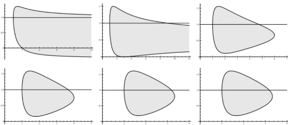
See Fig. 2.
As observed in [9, 14, 18], an improved inequality can also be obtained. Since the case p ∈ [1,2) is covered in Section 3, we shall assume from now on that p > 2. With ϕβ(s) = s Z 0 exp µ 2γ(β) β (β − 1) p ³¡ 1 − (p − 2) s¢1−ζ−21β−¡1 − (p − 2) z¢1−ζ−21β´¶d z ,
whereγ = γ(β) is given by (18) and ζ = ζ(β) =2−(4−p)β2β (p−2), let us consider ϕ(s) := supnϕβ(s) :β ∈B(p, d )
o
. (19)
Theorem 14. Let d ≥ 1 and assume that p ∈ (2,2∗). Inequality (5) holds withϕ
Proof. Using the identity12+β (p−2)β−1 + ζ = 1, Hölder’s inequality shows that 1 β2 Z Sd ¯ ¯∇¡uβ¢¯¯2dµ = Z Sd u2(β−1)|∇u|2dµ = Z Sd |∇u|2 u · u p(β−1) p−2 · u2βζdµ ≤ Z Sd |∇u|4 u2 dµ 1 2 Z Sd uβpdµ β−1 β (p−2) Z Sd u2βdµ ζ .
With the choice°°uβ°°Lp(Sd)= 1, we find that Z Sd |∇u|4 u2 dµ 1/2 ≥β12 ¡ i 1 − (p − 2)e¢ζ .
On the other hand, by using the identity12+β−12β +21β= 1, and Hölder’s inequality again, we have also
Z Sd |∇u|4 u2 dµ 1/2 ≥ R Sd|∇u|2dµ ¡ 1 − (p − 2)e¢21β ,
since dµ is a probability measure on Sd. Therefore, from (17) we get the inequality d
d t(i− de) ≤
γ(β)i e′
β2¡1 − (p − 2)e¢ζ+21β .
For everyβ > 1 it is possible to find a function ψβsatisfying the ODE ψ′′ β(s) ψ′ β(s) = −γ(β)β2 ¡ 1 − (p − 2) s¢−ζ−21β, ψ β(0) = 0,
withζ = ζ(β), such that ψ′
β> 0. Then d d t ¡i ψ′ β(e) − d ψβ(e)¢≤ 0,
from which we conclude thati≥ d ϕβ(e) withϕβ:= ψβ/ψ′
β. It is then elementary to
check thatϕβsatisfies the ODE ϕ′β= 1 − ϕβ ψ′′ β(s) ψ′ β(s) = 1 +γ(β) β2 ¡ 1 − (p − 2) s¢−ζ−21βϕ β
and thatϕβ(0) = 0. Solving this linear ODE, we find the expression of ϕβ. Notice that ϕβ is defined for any s ∈
£
0, 1/(p − 2)¢and thatϕβ(s) > 0 for any s 6= 0. From the
equation satisfied byϕβwe get thatϕ′β(s) > 1 and ϕ′′β(s) > 0, hence ϕβ(s) > s for any
Let us define µ(λ) = min t ≥1 · p − 2 t ϕ µ t − 1 p − 2 ¶ +λ t ¸ . (20)
By arguing exactly as in the proof of Theorem 2, we obtain an estimate of the optimal constant in (1) which is valid for instance if 2#< p < 2∗.
Corollary 15. Let d ≥ 1 and assume that p ∈ (2,2∗). With the notations of Theorem 14
andµ(λ) defined by (20), the optimal constant in (1) can be estimated for any p ∈ (2, 2∗) by
µ(λ) ≥ µ(λ) ∀λ ≥ 1.
Another consequence is that one can write an improved inequality on Rdin the spirit of Proposition 8, for any p ∈ (1,2∗), p 6= 2. Since the expression involves ϕ as defined
in Theorem 14, we do not get any fully explicit expression, so we shall leave it to the interested reader. A major drawback of our method is thatϕ is defined through a primitive. With some additional work,ϕ can be written as an incomplete Γ function, which is however not of much practical interest. This is why it is interesting to con-sider a special case, for which we obtain an explicit control of the remainder term. For completeness, let us state the following result which applies to a particular class of functions u.
Theorem 16 ([18]). Let d ≥ 3. If p ∈ (1,2) ∪ (2,2∗), we have
Z Sd |∇u|2dµ ≥ d p − 2 · 1 +(d 2− 4)(2∗− p) d (d + 2) + p − 1 ¸³ kuk2Lp(Sd)− kuk2L2(Sd) ´
for any u ∈ H1(Sd, dµ) with antipodal symmetry, i.e.,
u(−x) = u(x) ∀ x ∈ Sd. (21)
The limit case p = 2 corresponds to the improved logarithmic Sobolev inequality Z Sd |∇u|2dµ ≥d2(d + 3) 2 (d + 1)2 Z Sd |u|2log à |u|2 kuk2L2(Sd) ! dµ
for any u ∈ H1(Sd, dµ) \ {0} such that (21) holds.
We refer to [18, Theorem 5.6] and its proof for details. Instead of (21), one can use any symmetry which guarantees that d td RSdu(t , ·)β pdµ = 0 if we evolve u accord-ing to (15). Usaccord-ing the stereographic projection, one can obtain a weighted inequality with the same constant on Rd, for solutions which have the inversion symmetry cor-responding to (21).
5 Further results and concluding remarks
The interpolation inequalities (1) and (2) are equivalent to Keller-Lieb-Thirring es-timates for the principal eigenvalue of Schrödinger operators, respectively −∆ − V on Sdwith V ≥ 0 in Lq(Sd) for some q > 1, and −∆ + V on Sdwith V > 0 such that V−1∈ Lq(Sd), again for some q > 1. See for instance [13, 15] and references therein.
Corollary 17. Let d ≥ 1, q > max{1,d/2}, p = 2 q/(q − 1) and assume that V be a
positive potential in Lq(Sd) withµ = kV kLq(Sd). Ifλ(µ) denotes the inverse of λ 7→ µ(λ) defined by (20) for some convex function ϕ such that (5) holds with ϕ(0) = 0 and ϕ′(0) = 1, then λ1(−∆ −V ) ≥ −λ ¡ kV kLq(Sd) ¢ . Proof. From Hölder’s inequalityRSdV u2dµ ≤ µkuk2
Lp(Sd) with µ = kV kLq(Sd), we learn that R Sd ¡ |∇u|2−V u2¢dµ kuk2L2(Sd) ≥k∇uk 2 L2(Sd)− µkuk2Lp(Sd) kuk2L2(Sd) ≥ −λ(µ).
Corollary 17 applies toϕ defined by (19) for any p ∈ (2,2∗) and toϕ defined by (7) for
any p ∈ (2,2#). In that case, the result holds with
λ(µ) = µ if µ ∈ (0,1] and λ(µ) =p − 2 + γµ
1+p−2γ
p − 2 + γ if µ > 1.
Even more interesting is the fact that a result can also be deduced from Theorem 2 in the range p ∈ [1,2), p 6= p∗(d ), for which no explicit estimate was known so far. In
that case, let us define
λ(µ) = µ if µ ∈ (0,1] and λ(µ) =2 − p − γµ
1−2−pγ
2 − p − γ if µ > 1.
Corollary 18. Let d ≥ 1, q > 1, p = 2 q/(q + 1) and assume that V be a positive
poten-tial such that V−1∈ Lq(Sd). Then
λ1(−∆ −V ) ≥ λ¡kV kLq(Sd) ¢
.
Proof. By the reverse Hölder inequality, withµ =°°V−1°°−1Lq(Sd)we have Z
Sd ¡
The conclusion holds using (2) and Theorem 2, (i) .
Let us conclude with a summary and some considerations on open problems. This paper is devoted to improvements of (3) and (4) by taking into account additional terms in the carré du champ method. The stereographic projection then induces improved weighted inequalities on the Euclidean space Rd. Alternatively, various
improvements have been obtained on Rdusing the scaling invariance: see for in-stance [11] and references therein. It is to be expected that these two approaches are not unrelated as well as nonlinear diffusion flows on Sdand nonlinear diffusion flows on Rdcan probably be related. The self-similar changes of variables based on
the so-called Barenblatt solutions also points in this direction: see [17]. Concerning stability issues, we have been able to establish various estimates with explicit con-stants, which are all limited to the subcritical range p < 2∗when d ≥ 3. This is clearly not optimal (see [6, 18]). A last point deserves to be mentioned: improved entropy - entropy production estimates likei≥ d ϕ(e) mean increased convergence rates in
evolution problems like (11) or (15): how to connect an initial time layer with large entropyeto an asymptotic time layer with an improved spectral gap obtained, for
instance, by best matching (which amounts to impose additional orthogonality con-ditions for large time asymptotics), is a topic of active research.
Appendices
A Estimating the distance to the constants
In Section 1, we claimed that the entropy u 7→kuk
2
Lp(Sd)− kuk2L2(Sd) p − 2
is an estimate of the distance of the function u to the constant functions. Let us give some details. If p ∈ [1,2) we know that kuk2L2(Sd)− kuk2Lp(Sd)≥ 2 − p 2p−1p2kuk 2 (1−p) L2(Sd) Z Sd ¯ ¯|u|p − up¯¯ 2 pdµ p
with u = kukLp(Sd), for any u ∈ Lp∩ L2(Sd), by the generalized Csiszár-Kullback-Pinsker inequality: see [21, 8] or [10, Proposition 2.1], and references therein.
If p > 2, let us define the constant cq:= inf t ∈R+\{1} tq− 1 − q (t − 1) νq(t − 1) with νq(t ) = ( |s|2 if |s| ≤ 1 |s|q if s > 1 for any q > 1. Let q = p/2 and use the above constant to get, with t = u2/kuk2
L2(Sd), the estimate Z Sd |u|pdµ ≥ kukpL2(Sd) 1 +cp/2 Z Sd νp/2 Ã |u|2 kuk2L2(Sd) − 1 ! dµ
and deduce that
kuk2Lp(Sd)− kuk2L2(Sd)≥ kuk2L2(Sd) 1 +cp/2 Z Sd νp/2 Ã |u|2− u2 u2 ! dµ 2/p − 1
with u = kukL2(Sd), for any u ∈ Lp∩ L2(Sd). Although there is no good homogeneity property because of the definition of the functionνp/2, the right-hand side is clearly
a measure of the distance of u to the constant u.
B Stereographic projection
Let x ∈ Rd, r = |x|, ω = x
|x| and denote by (ρ ω, z) ∈ Rd× (−1,1) the cartesian
coordi-nates on the unit sphere Sd⊂ Rd +1given by z =r 2− 1 r2+ 1= 1 − 2 〈x〉2, ρ = 2 r 〈x〉2.
Let u be a function defined on Sdand consider its counterpart v on Rdgiven by
u(ρ ω, z) = µ 〈x〉2 2 ¶d −2 2 v(x) ∀ x ∈ Rd. Recall thatδ(p) = 2d − p (d − 2). For any p ≥ 1, we have
Z Sd |u|pdµ =¯¯Sd¯¯−12δ(p)2 Z Rd |v|p 〈x〉δ(p)d x and also Z Sd |∇u|2dµ +1 4d (d − 2) Z Sd |u|2dµ =¯¯Sd¯¯−1 Z Rd |∇v|2d x .
Acknowledgment: This work has been partially supported by the Project EFI (J.D., ANR-17-CE40-0030) of the French National Research Agency (ANR).
© 2019 by the authors. This paper may be reproduced, in its entirety, for non-commercial purposes.
References
[1] A. Arnold and J. Dolbeault. Refined convex Sobolev inequalities. J. Funct. Anal., 225 (2):337–351, 2005. URL http://dx.doi.org/10.1016/j.jfa.2005.05.003.
[2] D. Bakry and M. Émery. Diffusions hypercontractives. In Séminaire de
probabil-ités, XIX, 1983/84, volume 1123 of Lecture Notes in Math., pages 177–206. Springer,
Berlin, 1985. URL http://dx.doi.org/10.1007/BFb0075847.
[3] D. Bakry and M. Émery. Inégalités de Sobolev pour un semi-groupe symétrique. C. R.
Acad. Sci. Paris Sér. I Math., 301(8):411–413, 1985. ISSN 0249-6291.
[4] D. Bakry, I. Gentil, and M. Ledoux. Analysis and geometry of Markov diffusion
operators, volume 348 of Grundlehren der Mathematischen Wissenschaften [Fun-damental Principles of Mathematical Sciences]. Springer, Cham, 2014. URL https://dx.doi.org/10.1007/978-3-319-00227-9.
[5] W. Beckner. Sharp Sobolev inequalities on the sphere and the Moser-Trudinger in-equality. Ann. of Math. (2), 138(1):213–242, 1993. URL http://dx.doi.org/10.2307/ 2946638.
[6] G. Bianchi and H. Egnell. A note on the Sobolev inequality. J. Funct. Anal., 100(1): 18–24, 1991. URL https://dx.doi.org/10.1016/0022-1236(91)90099-Q.
[7] M.-F. Bidaut-Véron and L. Véron. Nonlinear elliptic equations on compact Riemannian manifolds and asymptotics of Emden equations. Invent. Math., 106(3):489–539, 1991. URL http://dx.doi.org/10.1007/BF01243922.
[8] M. J. Cáceres, J. A. Carrillo, and J. Dolbeault. Nonlinear stability in Lp for a confined
system of charged particles. SIAM J. Math. Anal., 34(2):478–494 (electronic), 2002. URL http://dx.doi.org/10.1137/S0036141001398435.
[9] J. Demange. Improved Gagliardo-Nirenberg-Sobolev inequalities on manifolds with positive curvature. J. Funct. Anal., 254(3):593–611, 2008. URL https://doi.org/10. 1016/j.jfa.2007.01.017.
[10] J. Dolbeault and X. Li. Φ-Entropies: convexity, coercivity and hypocoercivity for Fokker-Planck and kinetic Fokker-Planck equations. Mathematical Models and
Meth-ods in Applied Sciences, 28(13):2637–2666, 2018. URL https://doi.org/10.1142/
S0218202518500574.
[11] J. Dolbeault and G. Toscani. Stability results for logarithmic Sobolev and Gagliardo-Nirenberg inequalities. Int. Math. Res. Not. IMRN, 2016(2):473–498, 2016. URL http://dx.doi.org/10.1093/imrn/rnv131.
[12] J. Dolbeault, M. J. Esteban, M. Kowalczyk, and M. Loss. Sharp interpolation inequal-ities on the sphere: New methods and consequences. Chinese Annals of Mathematics,
Series B, 34(1):99–112, 2013. URL http://dx.doi.org/10.1007/s11401-012-0756-6.
[13] J. Dolbeault, M. J. Esteban, A. Laptev, and M. Loss. Spectral properties of Schrödinger operators on compact manifolds: Rigidity, flows, interpolation and
spec-tral estimates. Comptes Rendus Mathématique, 351(11–12):437 – 440, 2013. URL https://doi.org/10.1016/j.crma.2013.06.014.
[14] J. Dolbeault, M. J. Esteban, M. Kowalczyk, and M. Loss. Improved interpolation in-equalities on the sphere. Discrete and Continuous Dynamical Systems Series S
(DCDS-S), 7(4):695–724, August 2014. URL http://dx.doi.org/10.3934/dcdss.2014.7.695.
[15] J. Dolbeault, M. J. Esteban, and A. Laptev. Spectral estimates on the sphere. Analysis
& PDE, 7(2):435–460, 2014. URL https://doi.org/10.2140/apde.2014.7.435.
[16] J. Dolbeault, M. J. Esteban, and M. Loss. Nonlinear flows and rigidity results on compact manifolds. Journal of Functional Analysis, 267(5):1338 – 1363, 2014. URL http://dx.doi.org/10.1016/j.jfa.2014.05.021.
[17] J. Dolbeault, M. J. Esteban, and M. Loss. Interpolation inequalities, nonlinear flows, boundary terms, optimality and linearization. Journal of elliptic and parabolic
equa-tions, 2:267–295, 2016. URL http://dx.doi.org/10.1007/BF03377405.
[18] J. Dolbeault, M. J. Esteban, and M. Loss. Interpolation inequalities on the sphere: linear vs. nonlinear flows (inégalités d’interpolation sur la sphère : flots non-linéaires vs. flots linéaires). Annales de la faculté des sciences de Toulouse Sér. 6, 26(2):351–379, 2017. URL http://dx.doi.org/10.5802/afst.1536.
[19] J. Dolbeault, M. J. Esteban, M. Loss, and M. Muratori. Symmetry for extremal func-tions in subcritical Caffarelli–Kohn–Nirenberg inequalities. Comptes Rendus
Mathéma-tique, 355(2):133 – 154, 2017. URL http://dx.doi.org/10.1016/j.crma.2017.01.004.
[20] C. E. Mueller and F. B. Weissler. Hypercontractivity for the heat semigroup for ultras-pherical polynomials and on the n-sphere. J. Funct. Anal., 48(2):252–283, 1982. URL https://dx.doi.org/10.1016/0022-1236(82)90069-6.
[21] A. Unterreiter, A. Arnold, P. Markowich, and G. Toscani. On generalized Csiszár-Kullback inequalities. Monatsh. Math., 131(3):235–253, 2000. URL http://dx.doi.org/ 10.1007/s006050070013.
Figures
0.5 1.0 1.5 2.0 2.5 3.0 0.5 1.0 1.5 2.0 2.5 3.0Fig. 1. The best constant λ 7→ µ(λ) in Inequality (1) for d = 3 and p = 3 is represented by
the plain curve (numerical computation). The dashed line is the estimate of Proposition 10 (valid only for λ ≥ 1) and the dotted line is the estimate of Theorem 2.
2 4 6 8 10 0.5 1.0 2 4 6 8 10 12 0.5 1.0 1.5 1 2 3 4 5 6 7 0.5 1.0 1.5 1 2 3 4 5 0.5 1.0 1.5 1 2 3 4 0.5 1.0 1.5 1 2 3 4 0.5 1.0 1.5
Fig. 2. The admissible range for d = 1, 2, 3 (first line), and d = 4, 5 and 10 (from left to
right), as it is deduced from Lemma 13 using (16): the curves p 7→ m±(p)enclose the
admis-sible range of the exponent m.
Powered by TCPDF (www.tcpdf.org) Powered by TCPDF (www.tcpdf.org)