Public Spending Shocks in a Liquidity Constrained Economy
Edouard Challe Xavier Ragoty
December 2007
Abstract
This paper analyses the e¤ects of transitory increases in government spending when pub-lic debt is used as liquidity by the private sector. Aggregate shocks are introduced into an incomplete-market economy where heterogenous, in…nitely-lived households face occasionally binding borrowing constraints and store wealth to smooth out idiosyncratic income ‡uctua-tions. Debt-…nanced increases in public spending facilitate self-insurance by bond holders and may crowd in private consumption. The implied higher stock of liquidity also loosens the bor-rowing constraints faced by …rms, thereby raising labour demand and possibly the real wage. Whether private consumption and wages actually rise or fall ultimately depends on the relative strengths of the liquidity and wealth e¤ects that arise following the shock.
Keywords: Borrowing constraints; public debt; …scal policy shocks. JEL codes: E21; E62.
CNRS-DRM and University of Paris-Dauphine, 75775 Paris Cedex 16; [email protected].
Introduction
This paper analyses the e¤ects of transitory …scal expansions when public debt is used as liquidity by the private sector. We conduct this analysis in an incomplete-market model where agents face uninsurable idiosyncratic income risk and cannot borrow against future income (i.e., markets are ‘liquidity constrained’in the terminology of Kehoe and Levine, 2001 and others). Non-Ricardian models of this type have on occasion been used to analyse the aggregate and welfare e¤ects of public debt in the steady state (see Woodford, 1990; Aiyagari and McGrattan, 1998). To date, there have been surprisingly few attempts at clarifying how such economies respond to aggregate …scal shocks. One important contribution is Heathcote (2005), who o¤ers a quantitative assessment of the impact e¤ect of tax cuts. In this paper, we attempt to characterise analytically the impact and dynamic e¤ects of public-spending shocks on macroeconomic aggregates.
The spending shocks of which we analyse the e¤ects have one signi…cant (and realistic) feature: they are at least partly …nanced by government bond issues in the short run, with public debt then gradually reverting to some long-run target value thanks to future tax increases.1 Note that
whether public spending is …nanced by taxes or debt does not matter in complete markets, Ricardian economies with lump-sum taxation, because households’ discounted disposable income ‡ows are identical between alternative modes of government …nancing. Then, under reasonable assumptions about preferences and technology, the negative wealth e¤ects associated with transitory spending shocks lead to falls in the demand for both private consumption and leisure, which in turn produces a drop in the real wage (e.g., Baxter and King, 1993). However, the de…cit …nancing of spending shocks can have very di¤erent consequences when public debt is used as private liquidity, that is, as a store of value held by agents for precautionary purposes. Starting from a situation in which private liquidity is scarce (in a sense that we specify below), such policies have the side e¤ect of increasing the stock of liquidity available in the economy, thereby facilitating self-insurance by bond holders, and e¤ectively relaxing the borrowing constraints faced by households and …rms. As we show, the liquidity e¤ects associated with rising public debt tend to foster household private-consumption demand, along with the labour demand of borrowing-constrained …rms. Whether and when such liquidity e¤ects may o¤set wealth e¤ects, and thus overturn the predictions of the Ricardian model regarding the e¤ects of spending shocks on private consumption and wages, is the central theme of this paper.
1
Bohn (1998) established that the U.S. debt-GDP ratio is mean-reverting, due to the corrective action of the primary surplus. In their structural VAR analysis of …scal shocks, Blanchard and Perotti (2002) …nd a limited impact response of taxes to spending shocks, implying de…cit …nancing in the short run.
The market incompleteness-cum-borrowing constraint assumption is the only departure from the frictionless Ricardian framework considered here, the other aspects of our model remain fully standard in a stripped-down form. In contrast to several recent contributions on the e¤ect of public spending shocks, we thus assume that the labour and goods markets are perfectly competitive, that both nominal prices and wages are fully ‡exible, that utility is separable over time as well as over consumption and leisure at any point in time, that all agents are utility-maximising, that there are no externalities associated with public spending, and that taxes are lump sum. In particular, our results make clear that the pro-cyclical response of private consumption and wages after a …scal expansion may naturally arise from the non-Ricardian nature of the model alone, making other familiar imperfections, or various possible combinations of them, unnecessary.2
It is perhaps surprising that the actual impact of our …scal experiment is still subject to so much empirical controversy. In particular, the application of di¤erent identi…cation strategies to U.S. data has either supported the Ricardian prediction of a fall in private consumption and wages following an increase in public spending (Ramey and Shapiro, 1998; Ramey, 2007), or come to the opposite conclusion that both variables actually increase after the shock (e.g., Blanchard and Perotti, 2002; Perotti, 2007), which latter is consistent with the Old Keynesian model and with a version of the New Keynesian model endowed with a su¢ cient number of market imperfections (Gali et al., 2007). Given this lack of consensus, our goal here is not to take any strong position as to whether an adequate …scal policy model should generate pro- or counter-cyclical responses to public spending shocks. Rather, we use our model to show that both outcomes are theoretically possible (and not implausible quantitatively), depending on the relative strengths of the liquidity and wealth e¤ects that arise following the shock.
Our model belongs to the literature on the consequences of market incompleteness for …scal policy outcomes. Woodford (1990) and Aiyagari and McGrattan (1998) have considered optimal steady state public debt when the latter is held for self-insurance purposes. More recently, Angeletos and Panousi (2007) analysed the macroeconomic e¤ects of the size of the government in an
incom-2
Recent …scal policy models include Ravn et al. (2006), who assume imperfect competition together with habit formation over varieties of the consumption good, Linnemann (2006), who assumes that consumption and leisure are nonseparable while consumption is an inferior good, Linnemann and Shabert (2003), who have imperfect competition and sticky nominal prices, and Gali et al. (2007), who combine ad hoc ‘hand to mouth’ households with imperfect competition and price rigidities in both goods and labour markets. Papers analysing the e¤ects of distortionary taxation in the neoclassical growth model include Ludvigson (1996) and Burnside et al. (2004), while Baxter and King (1993) consider the e¤ects of gouvernment spending shocks when the latter generate external productivity e¤ects.
plete markets framework with Ricardian households and idiosyncratic production risk. Heathcote (2005) computed the e¤ect of temporary tax cuts when markets are liquidity constrained.
Section 1 introduces our basic liquidity-constrained economy, and Section 2 analyses the impli-cations of de…cit-…nanced public spending shocks on consumption and output. Section 3 introduces borrowing-constrained entrepreneurs, allowing us to study the e¤ect of aggregate liquidity on labour demand and the real wage. Section 4 summarises our results and discusses their robustness.
1
The model
The economy is populated by a government, as well as by a unit mass of in…nitely-lived households and a large number of …rms interacting in competitive goods and labour markets. Firms turn one unit of labour input, Lt; into one unit of output, Yt. Since Yt = Lt, the competitive wage rate is
constant and equal to 1. (Time-varying real wages will be introduced in Section 3, and the way in which capital accumulation might a¤ect our results is discussed in Section 4.)
1.1 Households
In every period, household i chooses consumption demand, cit; and labour supply, lit; in order to maximise Et 1 X j=0 j u ci t+j lit+j ; (1)
where 2 (0; 1) and u(c) is twice continuously di¤erentiable, and such that u0(c) > 0; u0(0) = 1, u00(c) < 0 and (c) cu00(c) =u0(c) 1.3
The status of individual households in the labour market randomly switches between employ-ment (during which they freely choose their labour supply) and unemployemploy-ment (in which they are excluded from the labour market). The idiosyncratic labour-income ‡uctuations that result are assumed to be entirely uninsurable (i.e., agents cannot issue assets contingent on their future employment status, and there are no unemployment bene…ts). Households’ asset wealth must be non-negative at all times, so that households cannot use private borrowing and lending to insulate individual consumption from idiosyncratic income ‡uctuations. Given these restrictions, the only way households can smooth consumption is by holding (riskless) government bonds. Household i
3
That (c) 1ensures that the substitution e¤ects do indeed dominate the income e¤ects (given a linear disutility of labour), so that the steady-state rate of interest increases with steady-state public debt.
thus faces the following budget and non-negativity constraints:
cit+ ait= ait 1Rt 1+ tilit Tt; (2)
cit 0; lti 0; ait 0: (3)
In equation (2), ait denotes the total quantity of bonds held by household i at the end of period t, Tt is a (possibly negative) lump-sum tax collected on all households at date t, Rt 1 is
the riskless gross interest rate on bonds from date t 1 to date t, and it is an indicator variable taking on the value 1 if the household is employed at date t and 0 otherwise. It is assumed that Prob t+1i = 1 ti= 1 = 2 (0; 1) and Prob t+1i = 0 ti= 0 = 0 (nothing substantial changes if we allow the probability of moving out of unemployment to be less than one, but the extra computations required make our results less transparent).
In general, uninsurable income risk generates in…nitely many household types, due to the de-pendence of current decisions on the household’s entire history of individual shocks. Here we focus on a particular equilibrium with a limited number of household types and a …nite-state wealth dis-tribution, allowing us to derive the model’s dynamics in closed form. We construct this equilibrium using a simple ‘guess and verify’ method based on two conjectures, and then derive a su¢ cient condition for both conjectures to hold in equilibrium once all their behavioural and market-clearing implications have been worked out.
The …rst conjecture (C1) is that the borrowing constraint is always binding for unemployed households. As such, unemployed households hold no government bonds at the end of the current period (i.e., they would like to borrow, rather than save), so that we can write from (2):
i
t= 0 ) cit= ait 1Rt 1 Tt; (4)
where ai
t 1is household i’s bond holdings inherited from the previous period (when this household
was employed). The second conjecture (C2) is that the borrowing constraint is never binding for employed households. From (1)–(2), the intratemporal optimality condition for any employed household i imposes that the marginal rate of substitution between leisure and consumption be equal to the real wage, so that we obtain:
i
t = 1 ) cit= u0 1(1) ce: (5)
Any employed household stays employed in the next period with probability and falls into un-employment with probability 1 . Conjecture C2 implies that employed households’consumption-savings plans are interior (i.e., ait > 0 if ti = 1) and, from (1), (4) and (5), that these plans obey
the following Euler equation:
1 = Rt+ (1 ) RtEtu0(aitRt Tt+1): (6)
The left-hand side of equation (6) is the current marginal utility of an employed household, u0(ce) = 1. The …rst part of the right-hand side of (6) is the discounted utility of a marginal unit of savings if the household stays employed in the next period (in which case u0(cit+1) = u0(ce) = 1), while the second part is the marginal utility of the same unit when the household falls into unemployment in the next period (i.e., becomes unemployed, liquidates assets and, from equation (4), enjoys marginal utility u0(cit+1) = u0(aitRt Tt+1)).
In equation (6), household i’s current asset demand only depends on aggregate variables (Rt
and Tt+1). The solution ait to (6) is thus identical across employed households and we can write: i
t = 1 ) ait= at(> 0): (7)
Equations (4) and (7) imply that all unemployed households (labelled ‘u-households’from now on) have identical consumption levels, so that their budget constraint becomes:
u : cut = at 1Rt 1 Tt: (8)
Employed households can be of two di¤erent types, depending on whether they were employed or not in the previous period. Call the former ‘ee-households’ and the latter ‘ue-households’. In the current period, ue-households consume ce and save at but enjoy no asset payo¤ (since they
were borrowing-constrained at date t 1 and thus chose ai
t 1= 0). Then, equations (2), (5) and
(7) yield the labour supply of ue-households, luet (which is homogenous across such households) as the residual of the following equation:
ue : ce+ at= ltue Tt: (9)
On the other hand, ee-households consume ce, save at, and enjoy the asset payo¤ at 1Rt 1.
This also uniquely de…nes their labour supply, lee
t ; through the following equation:
ee : ce+ at= at 1Rt 1+ ltee Tt: (10)
To summarise, C1 and C2 imply that households can be of three di¤erent types only (with budget constraints (8)–(10)), while the equilibrium wealth distribution is two-state (i.e., ait= at> 0
or 0). Given the assumed probabilities of changing employment status, the invariant proportions of u-, ee- and ue-households are (1 ) = (2 ), 1 2 and , respectively (i.e., the proportion of employed households is 1 2 + = 1 ). For simplicity, we assume that the proportion of each type of household is at the invariant distribution level from t = 0 onwards.
1.2 Government
Let Gt and Tt denote government consumption and lump-sum taxes during period t, respectively,
and Btthe stock of public debt at the end of period t. The government faces the budget constraint:
Bt 1Rt 1+ Gt= Bt+ Tt: (11)
In equation (11), we think of transitory variations in Gt as being exogenously chosen by the
government, of Bt as adjusting endogenously over time depending on the primary de…cit and the
equilibrium interest rate, and of Tt as obeying a …scal rule with feedback from macroeconomic
and/or …scal variables. Following the observation by Bohn (1998) that the US debt-GDP ratio is stationary, we restrict our attention to rules ensuring that public debt reverts towards its (ex-ogenous) long-run target B at least asymptotically. Such rules, which exclude Ponzi schemes, are consistent a wide variety of feedback mechanisms, including that from public debt to primary de…cit as in Bohn (1998), from output and debt to structural de…cits (e.g., Gali and Perotti, 2003), as well as from public debt and public spending to taxes (e.g., Gali et al., 2007). In Section 2 we illustrate the dynamic e¤ects of spending shocks under one of the simplest rules of this class.
1.3 Market clearing
In our economy, only employed households hold government bonds. Given the asymptotic distribu-tion of household types, the clearing of the bond, labour and goods markets requires, respectively:
(1 ) at= Bt; (12)
(1 2 ) leet + ltue= Lt; (13)
(1 ) ce+ cut + Gt= Yt: (14)
Substituting (5), (11) and (12) into the Euler equation (6), we may write the relation between the interest rate and …scal variables as follows:
Rt= 1 + (1 ) Etu0((2 ) (Bt+1 Gt+1+ Tt+1)) 1 (15)
Note that as ! 1 uncertainty regarding idiosyncratic labour income vanishes; the model then becomes Ricardian and Rt ! 1= , the gross rate of time preference. We may now state the
following existence proposition (the proof is found in Appendix A)
Proposition 1. Provided that ‡uctuations around the steady state are small, the three household type equilibria exist if and only if B 2 (0; B ), where B = u0 1(1) = (1 + ) (> 0). Along this equilibrium, Rt< 1= for all t.
In short, proposition 1 indicates that our economy is liquidity constrained if public debt is su¢ ciently low, in which case the equilibrium interest rate is also low (relative to that prevailing in an unconstrained economy).4 From now on we proceed under the maintained assumption that liquidity is scarce (in the sense that B 2 (0; B )), and defer until the last Section the discussion of the signi…cance of this assumption for our results.
2
Liquidity and wealth e¤ects of …scal expansions
2.1 Aggregate and individual variables
In this section we start by showing how liquidity and wealth e¤ects compete in determining the overall response of aggregate- and individual-level variables to public-spending shocks, and then illustrate the implied dynamic e¤ects of such shocks under a simple …scal rule.
Total consumption by employed households is (1 ) ce, while the total consumption of unem-ployed households is cu
t. Then, using (8), (11) and (12) and rearranging, total private consumption
and total output can be respectively written as:
Ct= (1 ) ce+ (1 ) (Bt Gt+ Tt) ; (16)
Yt= (1 ) ce+ (1 ) (Bt+ Tt) + Gt: (17)
Imagine …rst a rise in government consumption with a limited tax response in the short run, leading to rapid growth, and thus a persistently high stock, of public debt. This may cause the quantity Bt Gt+ Ttin (16) to be greater than zero over a sustained period of time starting at t+1,
thereby leading to persistent crowding-in of private consumption by public consumption (Figure 1.A. below illustrates this possibility). Alternatively, consider the pure Ricardian experiment of a debt-…nanced cut in lump-sum taxes, …nanced by future tax increases, with the entire path of government consumption remaining unchanged. Since Gt = 0 and thus Bt = Tt by
assumption, we have (Bt+ Tt) > 0 so that the cut raises private consumption and output on
impact. Finally, note that changes in taxes and public consumption that keep the primary de…cit at zero (that is, Gt = Tt and Bt= 0) a¤ect private consumption and output in exactly the
way predicted by the Ricardian model (i.e., Ct < 0, Yt > 0): variations in the stock of public
debt are thus crucial in generating the expansionary e¤ects of …scal shocks.
To obtain further insight into the underlying workings of these non-Ricardian e¤ects, we need to go beyond the reduced-form equations (16)–(17) and look at household-level variables, which
4
describe how individual consumption (i.e. the private demand side of the model) and labour supply (the supply side of the model) respond to …scal shocks. The consumption of employed households, ce, is not a¤ected by …scal shocks. Now, substitute (12) into (8) to write cut as follows:
cut = (2 ) Bt 1Rt 1 Tt: (18)
In equation (18), higher taxes lower consumption, but higher public debt raises the overall liquidation value of u-households’ portfolios (i.e., the (2 ) Bt 1Rt 1 term in (18)). Provided
that the increase in public debt also persistently raises the interest rate after the spending shock (which, from (15), occurs whenever Bt Gt+ Ttrises over time), the right-hand side of (18) may
increase. Ultimately, whether cu
t (and thus Ct) rises or falls thus depends on whether the liquidity
e¤ects of public debt on u-households’portfolios dominate the wealth e¤ects of taxes following the shock. Turning to the supply side of the model, we can substitute (5) and (12) into (9)–(10) and write labour supply by employed households as follows:
ltee= ce+ (2 ) (Bt Bt 1Rt 1) + Tt; (19)
luet = ce+ (2 ) Bt+ Tt: (20)
Equations (19)–(20) show that labour supply responds to both taxes (as in the Ricardian model) and the stock of liquidity that households acquire as self-insurance against unemployment risk. ue-households, who have just moved out of unemployment and have zero beginning-of-period wealth, will seize any extra opportunity to save by raising labour supply; ee-households, who are partly self-insured when they enter the current period, adjust their labour supply depending on the new stock of government bonds available for purchase relative to the current value of their previously-accumulated portfolio. In both cases, the growth of public debt that may result from higher public spending generates liquidity e¤ects that strengthen the wealth e¤ects on labour supply.
2.2 Dynamic e¤ects of public spending shocks: an example
Having discussed how liquidity e¤ects may a¤ect the response of our variables of interest to …scal expansions, we now illustrate the dynamics of the model in the context of a speci…c example of a …scal rule and a shock process. We assume here that Tt and Gt are given by:
Tt= T + (Bt B) ; (21)
Gt= Gt 1+ t; (22)
where T denotes steady-state taxes, > 0 and 2 (0; 1) are constant parameters, and tis a shock
expositional clarity and entails no loss of generality; here it implies that in the steady state tax revenues just cover interest rate payments on debt, i.e., T = B (R 1).5
The policy parameter e¤ectively indexes the way in which …scal expansions are …nanced at various horizons. If is large, taxes rise quickly following a …scal expansion and public debt plays a relatively minor rôle in their short-run …nancing. Smaller values of , on the contrary, imply a muted short-run response of taxes and a more substantial rôle for public debt issuance in the short run; the ensuing rise in the stock of public debt then eventually triggers a rise in taxes in the medium run until the reversion of the public debt has been completed. Of course, must be large enough to guarantee that public debt does not explode.6 Note that the qualitative properties of the model are robust to the inclusion of other feedbacks in (21), as well as to a lagged (rather than contemporaneous) reaction of taxes to public debt; what matters for our results is the possibility that public spending shocks entail changes in the stock of public debt, at least in the short run.
Substituting (21) into (11) and (15) and rearranging, we obtain a two-dimensional expectational dynamic system in Xt= [ Bt Rt ], with Gtas a forcing term and Ctand Ytgiven by (16)–(17). We
can then draw impulse-response functions using the VAR representation of the solution dynamics and the (quarterly) parameters = 0:98, = 0:94 (this generates an unemployment rate of
' 5:66%), = 0:95, the (unique) value of B such that R = 1:01, and u (c) = ln c:
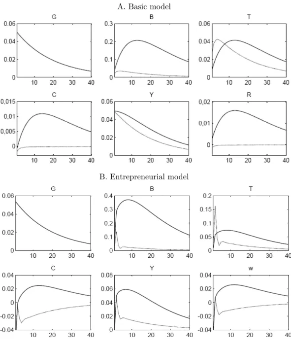
Figure 1.A. displays the responses of our variables of interest to a public-spending shock, when = 0:2 (the solid line) and = 1:2 (the dotted line). The case = 0:2 illustrates a situation where liquidity e¤ects dominate wealth e¤ects on private consumption (except at the very moment of the shock), due to the substantial increase in public debt and the implied improvement in households’ self-insurance opportunities (note that private consumption tracks public debt, and is thus far more persistent than the shock itself.) On the contrary, wealth e¤ects dominate when = 1:2, due to the small increase in public debt and the rapid reaction of taxes, resulting in a ‘Ricardian’ (i.e. negative) response of private consumption along the transition path. Holding other parameters constant, a sensitivity analysis indicates that values of between 0:2 and 1:2 cause consumption to fall below its steady-state level for several periods (during which public debt and implied liquidity e¤ects are still limited), and then rise above its steady-state level for the rest of the adjustment
5
As we show in appendix A, R 1may be negative if steady-state public debt is su¢ ciently low, in which case the steady state tax collection becomes a positive transfer T.
6Under (21), a necessary and su¢ cient condition for the existence and (local) stability of the equilibrium is:
> min=
R 1 + (2 )
1 (1 ) ; with =
(1 R) (cu)
1 + (1 ) R 2 (0; 1) ; and where, as is shown in Appendix A, R (> 0) is uniquely de…ned by B.
period (after public debt has risen enough to make the liquidity e¤ects prevalent). Since estimates of the response of taxes or the primary de…cit to public debt in U.S. post-war data indicate a slow reversion of public debt and a value of closer to 0:2 than to 1:2 (see Bohn, 1998, and Gali et al., 2007), plausible values of favour the dominance of liquidity e¤ects here, at least over part of the adjustment path.
A. Basic model
B. Entrepreneurial model
Figure 1. Dynamic effects of a public spending shock. The panels illustrate the linear deviations from the steady state of public debt (B), taxes (T), private consumption (C), output (Y) and the interest rate (R) or the wage rate (w), following a public spending shock (G) of 5% of steady-state output. The …scal rule isTt= T + (Bt B), with = 0:2(solid line) or = 1:2(dotted line).
3
Liquidity e¤ects on labour demand
Our analysis has thus far has focused on the way in which liquidity e¤ects may a¤ect the labour supply and consumption demand of private agents, leaving aside their potential e¤ects on labour demand and the equilibrium real wage. A simple way of introducing labour demand shifts into the basic model is to think of output as being produced by entrepreneurs, that is households having access to a production technology, rather than by a separate …rm sector. Higher liquidity may then also relax the borrowing constraints faced by these entrepreneurs and raise their labour demand following a …scal expansion. Here again, whether the real wage consequently rises or falls depends on whether the liquidity e¤ects on labour demand dominate the wealth e¤ects on labour supply following the …scal shock.
Our modi…ed model is exactly the same as that in Section 2 except for one feature: employed households now have a constant probability 1 of becoming entrepreneurs for exactly one period. Entrepreneurs have access to a production technology that yields yt+1i units of goods at date t+1 for lf;it units of labour hired at date t (entrepreneurs do not supply labour). The household’s objective is (1) as before, and we further assume here that u(c) = ln c, > 0. The budget constraint of household i is now:
cit+ ait+ 1 ti wtlf;it = at 1i Rt 1+ itwtlti+ yit Tt;
where ti = 1 if the household is employed and it= 0 if the household runs a …rm. Just as in Section 1, a limited number of household type/asset states equilibria can be constructed by conjecturing that employed households are never constrained while entrepreneurs always are. The resulting three household types are: i) entrepreneurs (or ‘f households’), who are currently borrowing-constrained and were employed in the previous period; ii) ee households, who are currently employed after having been employed in the previous period; and iii) f e households, who are currently employed after having been entrepreneurs in the previous period. Just as before, employed households are not borrowing-constrained and all choose the same consumption and asset holding levels, denoted by ce
t and at (cet will be time-varying here, due to changes in the real wage). We denote by c f t and
lft entrepreneurs’ consumption and labour demands, respectively. The budget constraint of each household type is now:
ee : cet + at= at 1Rt 1+ wtleet Tt; (23)
f e : cet + at= wtlf et + l f
t 1 Tt; (24)
Equation (23) is the same as (10), except for the fact that cet is time-indexed. In equation (24), f e-households earn labour income wtltf e plus production output yt= lt 1f ; and this total income is
used to pay for consumption, asset accumulation and taxes. Equation (25), the budget constraint of entrepreneurs, states that they entirely liquidate their stock of assets to …nance consumption, taxes, and the wage bill wtlft (i.e., they hold no bonds at the end of the period since they face binding
borrowing constraints). From (1) and the fact that employed households become entrepreneurs with probability 1 , the intratemporal and intertemporal optimality conditions of employed households are now, respectively:
wtu0(cet) = 1; (26)
u0(cet) = RtEt( u0 cet+1 + (1 ) u0(c f
t+1)): (27)
From (25), entrepreneurs must allocate their after-tax income, at 1Rt 1 Tt, to current
con-sumption, cft, and the wage bill, wtlft, taking the real wage as given. From (1), (24) and (25),
together with the fact that entrepreneurs stay so for one period only, the solution to the entrepre-neur’s choice must satisfy:
wtu0(cft) = Etu0 cet+1 : (28)
The optimality condition (28) simply sets equal the utility fall implied by a decrease in current consumption necessary to hire an extra unit of labour to the utility gain that is expected from increased current labour input (and thus future production) by that unit.
The market-clearing equations of the entrepreneurial model are as follows. Clearing of the market for bonds is given by equation (12) as before. Given that entrepreneurs are in proportion
; clearing of the labour and goods markets now requires:
(1 2 ) ltee+ lf et = lft; (29) (1 ) cet + cft + Gt= yt: (30)
Finally, the government’s behaviour is described by the budget constraint (11), together with our simple rule and shock process (21) and (22), where again is assumed to be large enough for public debt to be stationary. The necessary and su¢ cient condition for the existence of the three-type entrepreneurial economy is stated in the following proposition.
Proposition 2. Provided that ‡uctuations around the steady state are small, then the three household type equilibrium of the entrepreneurial model exists if and only if B 2 (0; B ), where B = 2( ( + 1 ) 1+ (1 ) 1): Along this equilibrium, R
The dynamic system characterising the entrepreneurial model involves more lags and more interactions between variables than the basic model, making it di¢ cult to compare directly the outcomes of the two models (the dynamic equations of the entrepreneurial model are stated in Appendix B). For the sake of comparability, we run policy experiments with exactly the same parameter values as in the previous Section, except for which is now set to 0.80 (this implies a share of entrepreneurs of ' 17%).7
Figure 2.B. displays the responses of …scal and aggregate variables to a public-spending shock generated by the entrepreneurial model (note that cet and lft, although not represented, are tracked by wt and Yt+1, respectively). Since liquidity e¤ects on labour demand take one period to be
operative (as some employed households having increased their savings turn into entrepreneurs), wealth e¤ects on labour supply dominate on impact whether = 0:2 or 1:2. The ensuing increase in labour supply leads to a sharp fall in the real wage and the consumption of employed households, causing total private consumption to fall. However, when = 0:2 liquidity e¤ects on labour demand become dominant (in the sense of leading to higher-than-steady-state wages) for the entire adjustment path starting from one period after the shock, leading to a persistent consumption boom. The responses of consumption and output are qualitatively similar to those in the basic model when = 1:2 (except for the initial wiggle due to the production delay), but labour-market adjustments matter here: the strong reaction of taxes and limited growth of public both act to weaken the liquidity e¤ects on labour demand whilst strengthening the wealth e¤ects on labour supply. This naturally leads to a limited increase in labour demand relative to the contemporaneous increase in labour supply, and thus to a fall in the real wage and a crowding out of private consumption by public spending. Just as in the basic model, intermediate values of generate a more mixed picture with dominance of either e¤ect at di¤erent points on the transition path.
4
Concluding remarks
This paper has presented the predictions of a liquidity-constrained economy regarding the e¤ects of debt-…nanced increases in public spending, with particular attention being paid to the e¤ects of such shocks on private consumption and the real wage. Our main point is to illustrate that the liquidity e¤ects induced by temporary changes in the stock of public debt can drastically alter the predictions of the baseline Ricardian model, where changes in public spending a¤ect aggregates only through
7
Our empirical counterpart to the share of entrepreneurs is the number of U.S. …rms, from The Census Bureau’s 2002 Survey of Business Owners (23 million …rms) divided by total employment by the end of the same year from the BLS Current Population Survey (136.5 millon people); 23=136:5 ' 0:17.
wealth e¤ects. The view that the de…cit …nancing of public spending can generate large multiplier e¤ects, thanks to consumption crowding-in, is often associated with the Keynesian tradition in macroeconomics; our model shows that such e¤ects are consistent with a set of assumptions (i.e., incomplete markets and borrowing constraints) that di¤er from typical Keynesian ones (e.g., sticky prices, imperfect competition).
We explore the implications of scarce liquidity for the transmission of …scal shocks using an extremely stylised model with limited agent heterogeneity and a limited number of assets. It is thus natural to wonder whether our results would still hold in a more realistic model allowing, for example, for more types of agents, or more types of liquid assets.
Our closed-form equilibrium results from the joint property that employed households reach their target precautionary wealth level instantaneously (an outcome of linear labour disutility), while unemployed households –or entrepreneurs–face a binding borrowing constraint and liquidate their asset portfolio from the very moment that their income falls. In a more general model with lower labour supply elasticity and slower asset liquidation, households would deplete or replete assets only gradually rather than in one go (e.g., Aiyagari and McGrattan, 1998; Heathcote, 2005), and the reactions of labour supply and consumption demand to changes in aggregate liquidity would be smoother. However, the same liquidity e¤ects of public debt should be at work (provided that agents e¤ectively use public debt as self-insurance), resulting in non-Ricardian e¤ects on total consumption, employment and wages. How wealth and liquidity e¤ects would quantitatively interact under gradual asset adjustment remains an open question that we leave for future research. Finally, our assumption that steady-state liquidity is scarce may be questioned on two grounds. First, are there no other means of self-insurance, like claims to the capital stock, that may lower the need for government-issued liquidity? Second, why should steady-state public debt be low, espe-cially when it may be Pareto-improving to increase its stock until full self-insurance is permitted? In our view, previous steady-state analyses provide answers to both questions. First, nothing guar-antees that capital alone can provide enough liquidity in steady state to mimic …rst-best outcomes, while the mere fact that capital is used as self-insurance turns the economy into a non-Ricardian one (Woodford, 1990); and in fact, our liquidity-constrained equilibrium survives endogenous cap-ital accumulation provided that steady-state capcap-ital (which depends, amongst other things, on the production function) is su¢ ciently low. Second, if taxes are distortionary rather than lump sum, increasing the public debt above a certain threshold may turn out to decrease, rather than increase, aggregate welfare (Aiyagari and McGrattan, 1998); in this situation, steady state public debt may endogenously be set by a benevolent government at a level where liquidity constraints still matter.
Appendix
A. Proof of Proposition 1
If ‡uctuations around the steady state are su¢ ciently small, then C1 and C2 hold in every period provided that they hold in the steady state. (12) implies that at> 0 if and only if Bt> 0, so C2
holds in the steady state if and only if B > 0. On the other hand, C1 holds in the steady state if and only if u0(cu) > Ru0(ce). From (5) and (8) we have u0(ce) = 1 and cu = aR T , so the latter inequality may be written as u0(aR T ) > R: Now, rewriting the steady-state counterpart
of (6) as
u0(aR T ) = (1 R) = ( R (1 )) ; (A1)
we …nd that the condition u0(cu) > Ru0(ce) is equivalent to R < 1= .
We now show that R < 1= if and only if B < B . This can be shown by …rst establishing that B is a continuous, strictly increasing function of R over the appropriate interval, and then by evaluating the function B (R) at the point R = 1= to …nd B . R is given by (15). By assumption G = 0, implying that T = B(R 1). Thus, after some manipulations the steady-state counterpart of (15) can be written as:
B = 1 1 + (1 ) Ru 0 1 ( R) 1 1 ! B (R) ; (A2)
where B (R) is positive and continuous over (0; 1= ). First, compute:
B0(R) = (1 ) (1 + (1 ) R)2 u 0 1 ( R) 1 1 ! + 1 1 + (1 ) R @ @Ru 0 1 ( R) 1 1 !
(A1) implies that u0(cu(R)) = (( R) 1 )= (1 ) ; so the @u0 1(:) =@R term above is: @ @Ru 0 1 ( R) 1 1 ! = 1 u00(cu) @u0(cu) @R = 1 u00(cu) 1 (1 ) R2:
After rearranging, this allows us to rewrite B0(R) as follows:
B0(R) = (1 ) c u (1 + (1 ) R)2 + R 2 (1 ) (1 + (1 ) R) 1 u00(cu) = (1 ) u 0(cu) (1 + (1 ) R)2u00(cu) (c u) 1=R + 1 (1 ) (1 R)
The term inside brackets must be negative for B0(R) to be positive. Since (c) 1 by assumption, a su¢ cient condition for this is that (1=R + 1 ) = (1 ) (1 R) > 1, which is always true. Thus, B (R) is continuous and strictly increasing in over (0; 1= ), while limR!0B = u0 1(1) (= 0 by assumption) and limR!1= B = u0 1(0) = ( + 1 ) ( 1). Then, setting R = 1= in (A2) gives B . Note also from (A2) that R < 1 if B < (2 ) 1u0 1 1 = (1 ) .
B. Proof of proposition 2
We must …rst derive the dynamic system characterising the entrepreneurial equilibrium under the joint conjecture that entrepreneurs are always borrowing-constrained while employed households never are, and then derive from the steady-state relations the range of debt levels compatible with this joint conjecture. With u (c) = ln c, equations (26) and (28) give:
cet = wt; cft = wt=( Et wt+11 ) (B1)
Substituting (B1) into (30), the goods-market equilibrium can be written as:
wt+ (1 ) wt=( Et wt+11 ) + (2 ) Gt= (1 ) lt 1f : (B2)
Substituting (11), (12) and (B1) into the budget constraint of f -households, (25), gives:
wt=( Et wt+11 ) + wtltf = (2 ) (Bt Gt+ Tt) : (B3)
Finally, substituting (B1) into (27), the Euler equations for employed households is:
wt1 = Rt Et wt+11 + (1 ) Et wt+11Et+1 wt+21 (B4)
Since shocks are small by assumption, the dynamic system just derived is an equilibrium if, in the steady state, i) all employed households hold positive assets at the end of the current period (which, from (12), is ensured by B > 0), and ii) entrepreneurs are always borrowing-constrained, i.e., u0(cf) > Ru0(ce). From (B1), this latter condition is equivalent to wR < 1. Now, the steady state counterpart of (B4) gives:
w = 2(1 ) R= (1 R) (B5)
Substituting (B5) into the inequality wR < 1, we …nd that entrepreneurs are borrowing-constrained if, and only if, R < 1= . We may now compute B ; the unique upper debt level en-suring that R 2 (0; 1= ) whenever B 2 (0; B ). First, use the facts that G = 0 and T = B (R 1) to write the steady-state counterparts of (B2) and (B3) as follows:
w= (1 ) + w2= = lf lf = B (1 + (1 ) R) =w w=
Equating the two and using (B5), we can write steady-state public debt as:
B (R) = R 1=R + 1 2(1 ) 1 R 2 1 1 + 1 + (1 ) R 1 R (B6)
B (R) is continuous and increasing in R over [0; 1= ) ; while B (0) = 0 and limR!1= B = 1. This uniquely de…nes B = B (1= ) in proposition 2.
References
Aiyagari, S. R. and McGrattan, E.R. (1998), The optimum quantity of debt, Journal of Monetary Economics, 42, 447-469.
Angeletos, G-M. and Panousi, V. (2007), Revisiting the supply-side e¤ects of government spending under incomplete markets, NBER Working Paper no 13136, October.
Baxter, M. and King, R.G. (1993), Fiscal policy in general equilibrium, American Economic Review, 83(3), 315-334.
Blanchard, O. and Perotti, R. (2002), An empirical characterization of the dynamic e¤ects of changes in government spending and taxes on output, Quarterly Journal of Economics, 113(3), 949-963.
Bohn, H. (1998), The behavior of US public debt and de…cits, Quarterly Journal of Economics, 117(4), 1329-1368.
Burnside, C., Eichenbaum, M. and Fisher, J.D.M. (2004), Fiscal shocks and their consequences, Journal of Economic Theory, 115, 89-117.
Gali, J., Lopez-Salidoz, J.D., Valles J. (2007), Understanding the e¤ects of government spending on consumption, Journal of the European Economic Association, 5(1), 227-270.
Gali, J. and Perotti, R. (2003), Fiscal policy and monetary integration in Europe, Economic Policy, 37, 533-572.
Heathcote, J. (2005), Fiscal policy with heterogeneous agents and incomplete markets, Review of Economic Studies, 72, 161-188.
Kehoe, T.J. and Levine, D.K. (2001), ‘Liquidity constrained markets versus debt constrained mar-kets’, Econometrica, 69(3), 575-598.
Linnemann, L. (2006), The e¤ects of government spending on private consumption: A puzzle?, Journal of Money, Credit and Banking, 38(7), 1715-1736.
Ludvigson, S. (1996), The macroeconomic e¤ect of government debt in a stochastic growth model, Journal of Monetary Economics, 38, 25-45.
Perotti, R. (2007), In search of the transmission mechanism of …scal policy, NBER Macroeconomics Annual, forthcoming.
Ramey, V.A. (2007), Identifying government spending shocks: It’s all in the timing, Working Paper. Ramey, V.A. and Shapiro, M.D. (1997), Costly capital reallocations and the e¤ects of government spending, Carnegie Rochester Conference on Public Policy, 48, 145-194.
195-218.