Lars Gr¨une∗ Mathematisches Institut Fakult¨at f¨ur Mathematik und Physik
Universit¨at Bayreuth 95440 Bayreuth, Germany [email protected]
Patrick Saint–Pierre
Centre de recherche Viabilit´e, Jeux, Contrˆole Universit´e Paris IX Dauphine
Place du Mar´echal de Lattre de Tassigny 75775 Paris Cedex, France
[email protected] May 19, 2005
Abstract: We apply set valued analysis techniques in order to characterize the input–to–state dynamical stability (ISDS) property, a variant of the well known input–to–state stability (ISS) property. Using a suitable augmented differential inclusion we are able to characterize the epigraphs of minimal ISDS Lyapunov functions as invariance kernels. This characterization gives new insight into local ISDS properties and provides a basis for a numerical approximation of ISDS and ISS Lyapunov functions via set oriented numerical methods.
AMS Classification: 93D30, 93D09, 34A40, 65P40
Keywords: input–to–state stability, invariance kernel, Lyapunov functions, set valued analysis, set oriented numerics
1
Introduction
The input–to–state stability property (ISS), introduced by E.D. Sontag in 1989 [12] and further in-vestigated in, e.g., [7, 13, 15], has by now become one of the most influential concepts in nonlinear stability theory for perturbed systems. The property generalizes the well known asymptotic stability property to perturbed systems of the type ˙x(t) = f (x(t), w(t)) by assuming that each trajectory ϕ satisfies the inequality
kϕ(t, x, w)k ≤ max{β(kxk, t), γ(kwk∞)} (1.1)
for suitable comparison functions β ∈ KL and γ ∈ K∞.1 For an overview of applications of the ISS
property we refer to the survey [14] and the references therin.
One of the main features of ISS is its representation by a suitable Lyapunov function, see [15]. The ISS property is equivalent to the existence of a continuously differentiable function V : Rn→ R satisfying
the bounds
kxk ≤ V (x) ≤ σ(kxk) (1.2)
∗
This research was done while the first author was a professeur invit´e at the Universit´e Paris IX Dauphine. The hospitality of all the members of the Centre de recherche Viabilit´e, Jeux, Contrˆole and its former head Jean–Pierre Aubin is greatfully acknowledged.
1
See Section 2 for a definition of these function classes which are standard in nonlinear stability theory.
for some σ ∈ K∞, and the decaying property
inf
γ(kwk)≤V (x)DV (x)f (x, w) ≤ −g(V (x)) (1.3)
for some g : R+0 → R+0 with g(r) > 0 for r > 0. This Lyapunov function characterization comes
in different variants, and the fact that we prefer this particular form lies in the fact that integrating (1.3) for some perturbation function w and using (1.2) one obtains (1.1) with γ from (1.3) and β(r, t) = µ(σ(r), t) where µ is the solution of the initial value problem ˙µ = −g(µ), µ(0) = r. Hence, the functions σ, γ and µ from V immediately carry over to the comparison functions in the ISS estimate (1.1).
A more careful investigation of this argument reveals that the existence of V with (1.2), (1.3) implies a slightly stronger property than ISS, namely the input–to–state dynamical stability property (ISDS) introduced in [4, Chapter 3] and [5] (see also [6]). The ISDS property, which will be precisely defined in Definition 2.1, below, is qualitatively equivalent to ISS (see [4, Proposition 3.4.4(ii)]) but, due to its tighter quantitative relation to V , more suitable for a Lyapunov function based analysis. Hence, in this paper we will work with this ISDS property which we will use in a rather general version by considering arbitrary compact sets A instead of the origin, and by allowing that ISDS only holds on a subset B ⊆ Rn instead of the whole Rn.
This paper deals with the characterization of the ISDS property and ISDS Lyapunov functions using set valued techniques. More precisely, to our n–dimensional perturbed system we associate an augmented n + 1–dimensional differential inclusion with solutions ψ, where the additional dimension represents the value of the Lyapunov function V . Via this inclusion we obtain a characterization of V via the invariance kernel Invψ(D) of a suitable set D. In particular, we are able to give a necessary and
sufficient condition on the shape of Invψ(D) being equivalent to the ISDS property. Furthermore,
the invariance kernel Invψ(D) characterizes the minimal ISDS Lyapunov function by means of its
epigraph, provided that ISDS holds. However, even when ISDS does not hold the set Invψ(D) may
contain useful information. If ISDS does not hold for some perturbation range W , then it may still hold for a suitably restricted perturbation range fW . It turns out that the invariance kernel Invψ(D)
for the unrestricted perturbation set W can be used in order to determine whether this is the case, and if so, then Invψ(D) gives a precise estimate about the size of the maximal restricted perturbation
range fW for which ISDS holds.
The contribution of these results is twofold. First, our results give additional insight into the ISDS (and thus the ISS) property and the respective Lyapunov functions. In particular, our second result characterizes the situation where ISDS is lost due to a too large set of perturbations, a topic which was recently investigated in [3] using a controllability analysis. Second, since invariance kernels are computable by set valued numerical algorithms, our characterization leads to a numerical approach for computing ISDS Lyapunov functions for which — to the best of our knowledge — no other numerically feasible representation is available until now. It goes without saying that the numerical effort of this approach is rather high such that our method is only applicable to moderately complex systems of low dimensions, but this is due to the inherent complexity of the problem, taking into account that the computation of nonlinear Lyapunov functions is a difficult task even for unperturbed systems. This numerical approach bears some similarities with a recently developed dynamic programming method for the computation of ISS comparison functions [8], with the difference that here Lyapunov functions are computed while in [8] the comparison functions (or gains) are obtained.
This paper is organized as follows. In the ensuing Section 2 we summarize the necessary background information on the ISDS property. In Section 3 we state and prove our first main result on the
representation of ISDS Lyapunov functions V via invariance kernels. Section 4 gives necessary and sufficient conditions for ISDS using a suitably restricted perturbation range. In Section 5 we present the numerical approach and finally, in Section 6, we show some examples.
2
Setup and preliminaries
We consider perturbed nonlinear systems of the form ˙
x(t) = f (x(t), w(t)) (2.1)
with x ∈ Rn, and w ∈ W := L
∞(R, W ) for some W ⊆ Rl. We assume that f is continuous and
Lipschitz in x uniformly for w in a compact set. We denote the solutions with ϕ(t, x, w). For a compact set A ⊂ Rn we denote the Euclidean distance to A by dA.
We define the comparison function classes
K := {α : R+0 → R+0 | α is continuous and strictly increasing with α(0) = 0}
K∞ := {α ∈ K | α is unbounded}
L := {α : R+0 → R +
0 | α is continuous and strictly decreasing with limt→∞α(t) = 0}
KL := {β : R+0 × R + 0 → R
+
0 | β is continuous, β(·, t) ∈ K, β(r, ·) ∈ L for all t, r ≥ 0}
KLD := {µ ∈ KL | µ(r, 0) = r, µ(r, t + s) = µ(µ(r, t), s) for all r, t, s ≥ 0}
The first four classes are standard in nonlinear stability theory while the last class KLD of “dynamical” KL functions was introduced in [4] in order to formalize the specific form of KL functions β(r, t) = µ(σ(r), t) originating from the integration of a Lyapunov function, cf. the introduction.
Using these functions we can now define the ISDS property.
Definition 2.1 The set A is called input–to–state dynamically stable (ISDS) on some open neighbor-hood B of A, if for suitable µ ∈ KLD and σ, γ ∈ K∞ and all x ∈ B, all w ∈ W and all t ≥ 0 the
inequality dA(ϕ(t, x, w)) ≤ max{µ(σ(dA(x), t), ν(w, t)} (2.2) holds with ν(w, t) := ess sup τ ∈[0,t] µ(γ(kw(τ )k), t − τ ). (2.3) We call A globally ISDS if this property holds with B = Rn.
The most important feature of the ISDS property is its quantitative characterization by an ISDS Lyapunov function. If B 6= Rn then for its definition we need the reachable set Rϕ,W(B) of a set B
under ϕ, defined by
Rϕ,W(B) := [
w∈L∞(R,W ),x∈B,t∈[0,Tmax(x,w))
{ϕ(t, x, w)},
Definition 2.2 A function V : Rϕ,W(B) → R is called an ISDS Lyapunov function, if it satisfies the inequalities V (x) ≥ dA(x) for all x ∈ Rϕ,W(B) V (x) ≤ σ(dA(x)) for all x ∈ B (2.4) and V (ϕ(t, x, w)) ≤ max{µ(V (x), t), ν(w, t)} (2.5) for all x ∈ Rn, w ∈ W and t ≥ 0 with ν from (2.3).
It is easily seen that the existence of V meeting Definition 2.2 implies ISDS with the same comparison functions. The converse is also true but much less trivial to prove, cf. [4, Theorem 3.5.3] or [5, Theorem 4]2. Thus, an ISDS Lyapunov function for given comparison functions µ, σ, γ exists if and only if the set A is ISDS for these comparison functions and the ISDS property admits a precise quantitative charactarization by ISDS Lyapunov functions.
In the remainder of this paper we will always assume that the function µ ∈ KLD satisfies the differential equation
d
dtµ(r, t) = −g(µ(r, t)) (2.6)
for some Lipschitz continuous g : R → R with g(r) > 0 for r > 0. By [4, Proposition B.2.3] this can be assumed without loss of generality, more precisely, for any given ˜µ ∈ KLD we find µ ∈ KLD arbitrarily close to ˜ν satisfying (2.6).
Remark 2.3 If the function V from Definition 2.2 is smooth and µ satisfies (2.6), then (2.5) is equivalent to the infinitesimal inequality (1.3), see [5, Lemma 15]. Even if V is not smooth one can use this infinitesimal characterization, when interpreted in the viscosity solution sense, see [4, Proposition 3.5.6] for details. In this paper, we will work directly with (2.5), thus avoiding the use of nonsmooth differential calculus.
3
An invariance kernel representation
Fixing two functions γ ∈ K∞and µ ∈ KLD satisfying (2.6), to our perturbed system (2.1) we associate
the n + 1–dimensional differential inclusion ˙ x(t) ∈ f (x(t), W (y(t))) ˙ y(t) = −g(y(t)) with W (y) = {w ∈ W | γ(kwk) ≤ y} (3.1)
and y ∈ R+0. We denote the solutions by ψ(t, x, y), by ψ(t, z) for z = (x, y) ∈ Rn+1 or simply by
ψ(t), if there is no ambiguity. We will frequently use the decomposition ψ(t) = (ψx(t), ψy(t)) with
ψx(t) ∈ Rn and ψy(t) ∈ R. We assume that the right hand side of this differential inclusion and the
map y W (y) are Lipschitz set valued maps, which holds, e.g., if W is a star shaped set and γ−1 is Lipschitz, which can be assumed without loss of generality.
2
In fact, in [5] only the special case A = {0} and B = Rn is treated, but the proof easily carries over to our more
The following sets will be crucial for our analysis.
For a subset D ⊂ Rn+1 and a differential inclusion with solutions denoted by ψ we define its (forward) invariance kernel as
Invψ(D) := {z ∈ D | ψ(t, z) ∈ D for all solutions ψ of (3.1) and all t ≥ 0}.
For an extended real valued function G : Rn→ R ∪ {∞} we define its epigraph Epi(G) ⊂ Rn+1 by
Epi(G) := {(x, y) ∈ Rn+1| y ≥ G(x)}. For a set B ⊆ Rn we define
Epi(G|B) := Epi(G) ∩ (B × R).
Since ISDS Lyapunov functions are in general only defined on subsets C ⊂ Rn we extend them to Rn by setting V (x) = ∞ for x 6∈ C and define Dom(V ) := {x ∈ Rn| V (x) < ∞}.
The set which we are interested in is the invariance kernel Invψ(D) of the set
D := Epi(dA) = {(x, y) ∈ Rn+1| y ≥ dA(x)}. (3.2)
More precisely, we will use the largest epigraph contained in Invψ(D). For this purpose, for a given
closed set E ⊂ Rn+1 we define the set
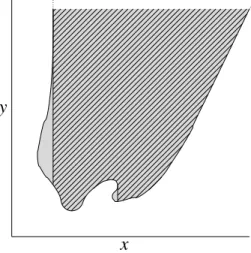
M(E) := {(x, y) ∈ E | (x, z) ∈ E for all z ≥ y}.
The set M(E) is the largest subset of E which can be written as an epigraph of a function G : Rn→ R ∪ {∞}. Figure 3.1 illustrates such a set.
x
y
Figure 3.1: Maximal epigraph M(E) (hatched) contained in a set E (gray)
Using these concepts we can now describe the relation between ISDS Lyapunov functions and suitable invariance kernels.
Theorem 3.1 Consider the perturbed system (2.1) and the differential inclusion (3.1). Consider a compact set A ⊂ Rn, an open neighborhood B ⊆ Rnof A and the set D from (3.2). Then the following assertions hold:
(i) Each ISDS Lyapunov function V : Rn→ R satisfies
Epi(V ) ⊆ M(Invψ(D)).
(ii) If there exists a function σ ∈ K∞such that
Epi(σ(dA)|B) ⊆ Invψ(D) (3.3)
holds, then there exists an ISDS Lyapunov function V : Rn→ R with
B ⊆ Dom(V ) and Epi(V ) = M(Invψ(D)).
In particular, this V is the minimal ISDS Lyapunov function for (2.1) in the sense that V (x) ≤ eV (x) holds for all x ∈ Dom(V ) and all other ISDS Lyapunov functions eV for the comparison functions µ and γ.
(iii) The set A is ISDS with neighborhood B if and only if (3.3) holds for some function σ ∈ K∞.
Proof: By [5, Lemma 13] a function V : R(B) → R satisfies (2.5) if and only if it satisfies V (ϕ(t, x, w)) ≤ µ(y, t) for all x ∈ B, all t ≥ 0, all y ≥ V (x)
and all w ∈ W with γ(kw(τ )k) ≤ µ(y, τ ) for almost all τ ∈ [0, t]. (3.4) For the sake of completeness we give the proof of the equivalence (2.5) ⇔ (3.4).
Assume (2.5) and w ∈ W is such that γ(kw(τ )k) ≤ µ(y, τ ) holds for almost all τ ∈ [0, t]. Then the definition of ν in (2.3) implies ν(w, t) ≤ µ(y, t), thus (2.5) immediately implies (3.4).
Conversely, assume (3.4) and consider w ∈ W, x ∈ B and t ≥ 0. Set y = max{V (x), µ(ν(w, t), −t)}, which by (2.3) implies γ(kw(τ )k) ≤ µ(y, τ ) for almost all τ ∈ [0, t], hence (3.4) implies V (ϕ(t, x, w)) ≤ µ(y, t). Now by the choice of y either y = V (x) or µ(y, t) = ν(w, t) holds. In the first case, from (3.4) we obtain V (ϕ(t, x, w)) ≤ µ(y, t) = µ(V (x), t) while in the second case we obtain V (ϕ(t, x, w)) ≤ µ(y, t) = ν(w, t). In both cases, (2.5) follows.
Using this equivalence we now turn to the proof of the theorem.
(i) Let (x, y) ∈ Epi(V ) and let ψ(t) = ψ(t, x, y) be a solution of the differential inclusion (3.1). We have to prove that (x, y) ∈ Invψ(D), i.e. ψ(t) ∈ D for all t ≥ 0. Writing ψ = (ψx, ψy) this amounts
to showing dA(ψx(t)) ≤ ψy(t) for all t ≥ 0. From Filippov’s Lemma (see [1] or [9, p. 267]) we find a
function w(t) with w(t) ∈ W (ψy(t)) for almost all t ≥ 0 such that ψx solves
d
dtψx(t) = f (ψ(x(t)), w(t)).
Since ψy(t) = µ(y, t) we obtain that γ(kw(τ )k) ≤ µ(y, τ ) for almost all τ ≥ 0. Thus from (3.4) we can
conclude V (ψx(t)) ≤ µ(y, t) which implies
i.e., ψ(t) ∈ D and thus (x, y) ∈ Invψ(D).
(ii) We show that the function V (x) defined by
V (x) := inf{y ≥ 0 | (x, y) ∈ M(Invψ(D))}
(with the convention inf ∅ = ∞) is an ISDS Lyapunov function. Clearly, the inequalities (2.4) follow immediately from the construction and (3.3). It remains to show (2.5) for x ∈ B which we do by verifying (3.4) for x ∈ Dom(V ). Consider t ≥ 0, x ∈ Dom(V ), w ∈ W. Then we find y ≥ 0 with (x, y) ∈ Invψ(D) such that γ(kw(τ )k) ≤ µ(y, τ ) holds for almost all τ ∈ [0, t]. The choice of y implies
that w(τ ) ∈ W (µ(y, τ )) for almost all τ ∈ [0, t], hence ψ(τ ) := (ϕ(τ, x, w), µ(y, τ )) is a solution of the inclusion on [0, τ ]. Since Invψ(D) is forward invariant we obtain ψ(τ ) ∈ Invψ(D) for all τ ∈ [0, t], in
particular ψ(t) ∈ Invψ(D). From the definition of V we obtain
V (ϕ(t, x, w)) ≤ µ(y, t), i.e. (3.4) which shows that V is an ISDS Lyapunov function.
The fact that this V is minimal follows immediately from (i), because each ISDS Lyapunov function V satisfies Epi(V ) ⊆ M(Invψ(D)), hence the one satisfying Epi(V ) = M(Invψ(D)) must be the minimal
one.
(iii) If the condition (3.3) holds, then by (ii) we obtain the existence of an ISDS Lyapunov function with Dom(V ) ⊇ B, hence ISDS on B. Conversely, if ISDS holds, then by [5, Theorem 4] there exists an ISDS Lyapunov function on B, thus from (i) we can conclude that Invψ(D) contains an epigraph
containing the points (x, V (x)) for x ∈ B, thus for σ ∈ K∞ from (2.4) Invψ(D) contains the points
(x, σ(dA(x))) for x ∈ B. Hence (3.3) follows.
Remark 3.2 The condition (3.3) involving σ implies that M(Invψ(D)) is not empty, that V is
con-tinuous at ∂V and that V is bounded on compact sets. Thus, it guarantees the existence of a function V with Epi(V ) = M(Invψ(D)) as well as some regularity properties of V . The inequality (2.5) is then
a consequence of the structure of the differential inclusion (3.1).
A particular nice situation occurs when Invψ(D) = M(Invψ(D)). In this cas we can state the following
corollary.
Corollary 3.3 Consider the perturbed system (2.1) and the differential inclusion (3.1). Consider a compact set A ⊂ Rn, an open neighborhood B ⊆ Rn of A and the set D from (3.2).
Assume that there exists a function V : Rn→ R ∪ {∞} and a function σ ∈ K∞ such that
Epi(σ(dA)|B) ⊆ Epi(V ) = Invψ(D)
holds. Then V is an ISDS Lyapunov function on B and, in particular, the set A is ISDS with neighborhood B.
Proof: Follows immediately from Theorem 3.1 (ii).
Note that the equality M(Invψ(D)) = Invψ(D) need not hold, even if M(Invψ(D)) 6= ∅, see Example
6.1, below. Hence, Corollary 3.3 indeed describes a special situation which can, hovewer, be observed for many systems.
4
ISDS for restricted perturbation range
Observe that Invψ(D) for D = Epi(dA) may be empty, even when no perturbations are present, e.g.,
when the set A is not forward invariant, like the set A = {1} for the simple 1d system ˙x(t) = x(t). Whenever A is forward invariant under ϕ for w ≡ 0 is is easily seen that Invψ(D) contains at least
the set A × {0}.
By Theorem 3.1 (iii), both Invψ(D) = ∅ and Invψ(D) = A × {0} imply that ISDS does not hold.
However, the converse is not true, i.e., if ISDS does not hold then Invψ(D) might still be nonempty
and strictly larger than A × {0}. As an example, consider the 1d system ˙
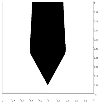
x(t) = −x(t)(1 − 2x(t)) + w(t). (4.1) We have computed the invariance kernel of D for A = {0} (i.e., dA = k · k is the Euclidean norm),
µ(r, t) = e−t/10r (i.e., d/dt µ(r, t) = −1/10 µ(r, t)), γ(r) = 2r (i.e., γ−1(r) = r/2), and W = R, using the numerical technique described in the following section. Figure 4.1 shows the numerically computed result.
Figure 4.1: Numerically determined invariance kernel Invψ(D) for System (4.1), W = R
Note that due to Theorem 3.1(iii) ISDS cannot hold because Invψ(D) does not contain an epigraph
for any neighborhood B of A = {0}, i.e., M(Invψ(D)) = ∅. The fact that the system is not ISDS can
also be seen directly, because it is easily verified that for x = 0 and, e.g., w ≡ 2 the corresponding trajectory grows unboundedly, it even tends to ∞ in finite time.
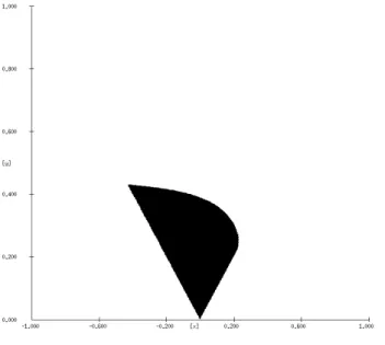
This gives rise to the question about the meaning of this nontrivial invariance kernel. The answer can be given when looking at the set W of admissible perturbation values. In fact, the shape of the invariance kernel in Figure 4.1 still contains what could be called a restricted epigraph, i.e., a set of the form Epi(V ) ∩ (Rn× [0, ˆy]) for some function V and some ˆy > 0. It turns out that choosing the “right” ˆy with this property, we can prove ISDS for a suitably restricted set fW ⊂ W of perturbation values. In order to make this statement precise and to formulate a necessary and sufficient condition
we need the horizontal cross section
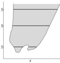
S(Invψ(D), y) := {x ∈ Rn| (x, y) ∈ Invψ(D)} of the set Invψ(D) ⊂ Rn+1, see Figure 4.2 for an illustration.
x
y
y
y
2 1 3Figure 4.2: Three cross sections S(E, yi), i = 1, 2, 3, (black) for the set E (gray) from Figure 3.1
These cross sections are subsets of Rn, and for such subsets S ⊆ Rnwe can define the invariance kernel under the solutions ϕ of (2.1) with perturbations from W ⊂ Rl by
Invϕ,W(S) := {x ∈ S | ϕ(t, x, w) ∈ S for all w ∈ L∞(R, W ), x ∈ S, t ≥ 0}.
Theorem 4.1 Consider a compact set A ⊂ Rn and the set Invψ(D) for D from (3.2).
(i) Assume that for some real number ˆy > 0 and the perturbation range fW := {w ∈ W | γ(kwk) ≤ ˆy} the set
C = Invϕ,fW(S(Invψ(D), ˆy))
contains a neighborhood B of A for which we can find a σ ∈ K∞ with the property
Epi(σ(dA)|B) ∩ (Rn× [0, ˆy]) ⊆ Invψ(D) (4.2)
Then the set A is ISDS with neighborhood B and perturbation range fW .
(ii) Conversely, if the set A is ISDS on some neighborhood B for the perturbation range fW = {w ∈ W | γ(kwk) ≤ ˆy} for some ˆy > 0, then the assumptions in (i) are satisfied for this value ˆy and C = Rϕ,fW(B).
Proof: (i) We prove the assertion by showing that for the differential inclusion ˙ x(t) ∈ f (x(t), fW (y(t))) ˙ y(t) = −g(y(t)) with fW (y) = {w ∈ fW | γ(kwk) ≤ y} (4.3)
with solutions denoted by ˜ψ the forward invariance kernel Invψ˜(D) satisfies (3.3) for B. Then (i)
follows from Theorem 3.1(iii).
We prove (3.3) using the forward invariance of C under ϕ and fW . This property implies ˜ψx(t, x, ˆy) ⊂ C
for all t ≥ 0 and all x ∈ C. In order to show (3.3), we have to show that for any point (x, y) with x ∈ B, y ≥ σ(dA(x)) and any solution ˜ψ(t) starting from this point the property ˜ψ(t) ∈ D holds for
all t ≥ 0. In order to accomplish this we show
there exists ˆt ≥ 0 with ˜ψ(t) ∈ D for all t ∈ [0, ˆt] and ˜ψ(ˆt) ∈ Invψ(D). (4.4)
This will prove (3.3) since Invψ(D) ⊆ D is forward invariant (4.3), due to the fact that the solution
set of (4.3) is smaller than that of (3.1),
If y ≤ ˆy then (4.2) implies (x, y) ∈ Invψ(D), hence (4.4) holds for ˆt = 0. If y > ˆy then we write
the solution as ˜ψ(t) = ( ˜ψx(t), ˜ψy(t)). Then the forward invariance of C under ϕ carries over to ˜ψx,
i.e., ˜ψx(t) ∈ C for all t ≥ 0. Since ˜ψy(t) → 0 we obtain ˜ψy(ˆt) = ˆy for some ˆt ≥ 0 and consequently
˜
ψ(ˆt) ∈ C ⊂ Invψ(D). For t ∈ [0, ˆt] we have ˜ψy(t) ≥ ˆy ≥ σ(dA( ˜ψx(t))), where the last inequality holds
because the point ( ˜ψx(t), ˆy) lies in C × {ˆy} ⊆ Invψ(D) ⊆ D = Epi(dA). Thus, ˜ψ(t) ∈ Epi(dA) = D,
which proves (4.4) in this case.
We have thus shown that Invψ˜(D) satisfies (3.3). This finishes the proof of (i) because now the ISDS
property follows immediately from Theorem 3.1(iii).
(ii) If ISDS holds for fW on some neighborhood B of A, then for this set of perturbations there exists an ISDS Lyapunov function V : Rϕ,fW(B) → R whose epigraph by Theorem 3.1(i) satisfies Epi(V ) ⊆ Invψ(D) and Epi(σ(dA)|B) ⊆ Epi(V ) for some σ ∈ K∞. Since R(B) ⊆ S(Invψ˜(D), ˆy) holds,
the invariance kernel Invψ˜(D) satisfies the assumptions from part (i). We have to show that Invψ(D)
also satisfies this assumptions, which we do by showing that these sets coincide for y ≤ ˆy. To this end consider the perturbation range W ⊇ fW . Then for any point (x, y) with y ≤ ˆy the set of possible solutions of (3.1) coincides with that of (4.3), because we have W (ψy(t)) ⊆ fW for all t ≥ 0. Hence we
have
Invψ˜(D) ∩ (Rn× [0, ˆy]) = Invψ(D)
which shows that the assumptions from (i) also hold for Invψ(D).
Remark 4.2 The equivalence of ISDS with fW and the condition in Theorem 4.1(i) implies that the maximal ˆy satisfying this condition characterizes the maximal set of perturbations for which ISDS holds for the considered comparison functions γ and µ.
Unfortunately, the first condition of Theorem 4.1(i), i.e., the assumption on the invariance kernel Invϕ,fW(S(Invψ(D), ˆy)) is not directly related to the shape of the invariance kernel Invψ(D), hence
just by looking at Invψ(D) it is not possible to verify the assumptions of Theorem 4.1(i).
Fortunately, there is a remedy to this problem if one aims at a sufficient ISDS condition analogous to Corollary 3.3. This corollary can be extended to the ˆy–restricted case without making assumptions on Invϕ,fW(S(Invψ(D), ˆy)). The key observation for this result is the following lemma, which gives a
Lemma 4.3 Assume that there exists ε > 0 such that the condition S(Invψ(D), y) ⊆ S(Invψ(D), ˆy)
holds for all y ∈ (ˆy − ε, ˆy) and some ˆy > 0. Then
Invϕ,fW(S(Invψ(D), ˆy)) = S(Invψ(D), ˆy)
for the perturbation range fW = {w ∈ W | γ(kwk) ≤ ˆy}.
Proof: We abbreviate C := S(Invψ(D), ˆy) and show that C is forward invariant for all perturbation
functions w ∈ W with α := γ(kwk∞) < ˆy. By continuity this implies the desired result also for α = ˆy.
Consider a point x ∈ C and a perturbation function w ∈ fW with α < ˆy. We prove the forward invari-ance by contradiction. For this purpose assume that there exists a time t > 0 such that ϕ(t, x, w) 6∈ C. Consider a time ∆t > 0 with the property that µ(ˆy, ∆t) > max{α, ˆy − ε}, which exists by continuity of µ and since ˆy > α. Since ϕ starts in C we find a time t1 ≥ 0 with
ϕ(t1, x, w) ∈ C and ϕ(t1+ ∆t, x, w) 6∈ C.
From the choice of ∆t we obtain kw(t)k ≤ µ(y∗, t) for almost all t ∈ [0, t1 + ∆t]. Hence, for t ∈
[t1, t1 + ∆t] the function ψ(t) = (ϕ(t, x, w), µ(y∗, t)) is a solution of the differential inclusion (3.1).
Furthermore, by the definition of y∗ the point (ϕ(t1, x, w), ˆy) lies in Invψ(D). Thus, the forward
invariance of Invψ(D) implies ψ(t1 + ∆t) ∈ Invψ(D) which in particular yields ϕ(t1 + ∆t, x, w) ∈
S(Invψ(D), µ(ˆy, ∆t) ⊆ C which contradicts the choice of t1 and ∆t. Thus C is forward invariant
under ϕ.
Using this fact we can state the following result, which is analogous to Corollary 3.3.
Corollary 4.4 Consider the perturbed system (2.1) and the differential inclusion (3.1). Consider a compact set A ⊂ Rn, an open neighborhood B ⊂ Rn of A and the set D from (3.2).
Assume that there exists a function V : Rn→ R ∪ ∞, a function σ ∈ K∞ and a value ˆy > 0 such that
Epi(σ(dA)|B) ∩ (Rn× [0, ˆy]) ⊆ Epi(V ) ∩ (Rn× [0, ˆy]) = Invψ(D) ∩ (Rn× [0, ˆy])
holds. Then V is an ISDS Lyapunov function on B for the perturbation range fW = {w ∈ W | γ(kwk ≤ ˆ
y}. In particular, the set A is ISDS with neighborhood B for perturbation range fW . Proof: From Epi(V ) ∩ (Rn× [0, ˆy]) = Inv
ψ(D) ∩ (Rn× [0, ˆy]) we obtain the equality
S(Invψ(D), y) = V−1([0, y])
for all y ∈ [0, ˆy]. This immediately implies S(Invψ(D), y1) ⊆ S(Invψ(D), y2) if 0 ≤ y1 ≤ y2 ≤ ˆy, hence
by Lemma 4.3 we obtain Invϕ,fW(S(Invψ(D), ˆy)) = S(Invψ(D), ˆy). Thus, Theorem 4.1 (i) yields the
assertion.
We can apply this result to our Example (4.1) with Invψ(D) from Figure 4.1. There one sees that the
condition of Corollary 4.4 is satisfies e.g. for ˆy = 0.24. Note that for large ˆy the assumed epigraph property from Corollary 4.4 is not satisfied and the inclusion S(Invψ(D), y) ⊆ S(Invψ(D), ˆy) for y < ˆy
does not hold. Since γ(r) = 2r, we obtain ISDS with fW = [−0.12, 0.12]. The numerical computation of the corresponding invariance kernel Invψ˜(D) as shown in Figure 4.3 indicates that this is the case
Figure 4.3: Numerically determined invariance kernel Invψ˜(D) for System (4.1), fW = [−0.12, 0.12]
5
Numerical techniques
Both systems (3.1) and (4.3) can be written as a differential inclusion system X0 ∈ F (X)
where X := (x, y) and F (X) = {(f (x, w), −g(y)), where w ∈ W (y) or w ∈ fW (y)}.
Looking for the invariance kernel of the set D := Epi(dA) = {(x, y) ∈ Rn+1| y ≥ dA(x)}, we consider
the viability kernel algorithm introduced in [11], extended in [2] to differential games for computing discriminating kernels for two players’ games, and reduced to “single second player’s game” since, in the absence of control, i.e., in the absence of the first player, the problem of finding discriminating kernels reduces to finding invariance kernels.
We do not intend to give a complete description of this algorithm but we recall its main features and refer to [2] for details.
Let M := supY ∈F (X), X∈DkY k and B the unit ball of Rn+1 which for simplicity we take of the form
B := Bx× [−1, +1].
Let us fix a time step ρ and let Fρ(X) be a suitable approximation of F satisfying
i) Graph(Fρ) ⊂ Graph(F ) + M ρB
ii) S
Z∈B(X,M ρ)F (Z) ⊂ Fρ(X) . (5.1)
For instance when F is `–Lipschitz and M –bounded, then the set valued map Fρ defined by Fρ(X) :=
F (X) +12M `ρB satisfies properties (5.1 i) and ii)).
Discretization in time
Replacing the derivative X0(t) of X at time t by the difference Xn+1ρ−Xn where Xn stands for X(nρ)
consider the recursive inclusion
Xk+1∈ Gρ(Xk) (5.2)
The discrete invariance kernel of D for Gρ, denoted
−−→
InvGρ(D), is the largest closed subset of initial
positions contained in D from which all solutions of the discrete inclusion (5.2) remain in D forever. Let us recall that the discrete viability kernel of D for Gρ, denoted
−−→
ViabGρ(D), is the largest closed
subset of initial positions contained in D from which at least one solution to the discrete inclusion (5.2) remains in D forever.
The invariance kernel algorithm consists of the construction of a decreasing sequence of subsets Dρk recursively defined by
D0ρ= D, and Dρk+1= Dρk∩ {X | Gρ(X) ⊂ Dρk}. (5.3) This algorithm allows to approximate the invariance kernel.
Theorem 5.1 Let F be a Lipschitz, convex and compact set valued map on a compact set D, Fρan
approximation of F satisfying (5.1) and Gρ:= Id + ρFρ. Then
Dρ:= lim k→+∞D k ρ = −→ InvGρ(D). lim ρ→0 −→ InvGρ(D) = InvF(D)
These convergence properties follow from general convergence theorems that can be found in ([2], Theorem 4.8, p. 218 and Theorem 4.11, p. 221).
Discretization in space
Considering a grid Xh := (hZ)n associated with a state step h, we define the projection of any set
E ⊂ Rn on Xh as follows:
Eh := (E + hB) ∩ Xh.
Then the fully discrete invariance kernel algorithm reads D0ρh= Dh, and Dρhk+1= D
k
ρh∩ {Xh | Gρh(Xh) ⊂ Dρhk } (5.4)
where Gρh(Xh) := (Xh+ ρFρ(Xh) + hB) ∩ Xh.
Let us just mention that, on the one hand, the choice of the time step ρ may depend on X and that, on the other hand, there exists a refinement principle which allows to restart the computation from a neighborhood of−→InvGρh(Dρh) instead of Dρh/2 when dividing the state step h by 2.
Functional approximation
In general the invariance kernel is not the epigraph of a function from Rn to R. However, when it is, as it may happen in the case of ISDS Lyapunov functions, we can derive from the invariance kernel algorithm a “functional approximation” of the invariance kernel, i.e., instead of the whole set Inv(D) we approximate a function Φ with Inv(D) = Epi(Φ). Let
Φ0ρ(x) := dA(x)
and consider the sequence of functions Φkρ defined on Rn as Φk+1ρ (x) = min{y ≥ Φkρ(x) | y ≥ sup w∈W (y),bx∈Bx Φnρ(x + ρ(f (x, w) + 1 2M `ρbx)) + ρg(y) + 1 2M `ρ 2}
Proposition 5.2 If the sets Dk
ρ from (5.3) are epigraphs then the sequence of function Φkρ converges
pointwisely to a function Φ∝ when k → ∞ and ρ → 0 satisfying Epi(Φ∝) = InvF(D)
Proof: This proposition is derived from Theorem 5.1 by induction over k. For k = 0 we have Epi(Φ0ρ) = Dρ0. Let us assume that Epi(Φkρ) = Dkρ. From the definition of Dk+1ρ , (x, y) ∈ Dρk+1 if and only if (x, y) ∈ Dkρand ∀w ∈ W (y), ∀(bx, by) ∈ B, (x+ρ(f (x, w)+12M `ρbx), y−ρ(g(y)+12M `ρby)) ∈ Dkρ.
In other words, (x, y) ∈ Dk+1ρ if and only if
y ≥ Φkρ(x) and y ≥ sup w∈W (y),bx∈Bx Φkρ(x + ρ(f (x, w) + 1 2M `ρbx)) + ρg(y) + 1 2M `ρ 2.
If Dk+1ρ is an epigraph then the set of y satisfying these inequalities is of the form [y∗, ∞) with y∗being the minimal y satisfying these inequalities. Thus, the definition of Φk+1ρ yields Dρk+1= Epi(Φk+1ρ ). Now pointwise convergence follows from the fact that the sets Dρk are decreasing in k and increasing in ρ. Hence the function Φkρ is monotone in these parameters which implies convergence.
Remark 5.3 In general, the problem of finding y meeting the two inequalities in the previous proof may have no solution. In this case the set Dρk+1 cannot have an epigraphic representation which is the case, e.g., for the system (3.1) where the perturbation range depends on y. When considering the restricted perturbation range fW instead of W , then for y ≥ ˆy the second inequality becomes
y − ρg(y) ≥ sup w∈fW (ˆy),bx∈Bx Φkρ(x + ρ(f (x, w) +1 2M `ρbx)) + 1 2M `ρ 2
so that if the map y → y − ρg(y) is increasing, then the minimal value y∗for y exists and, if it is larger than ˆy, it is given by the explicit formula
y∗ = Φn+1ρ (x) := (Id − ρg)−1( sup w∈fW (ˆy),bx∈Bx Φkρ(x + ρ(f (x, w) + 1 2M `ρbx)) + 1 2M `ρ 2).
6
Examples
In this section we provide two examples illustrating our theory and our numerical approach.
The first example is motivated by a question which arises when looking at our results: is it possible that Invψ(D) contains a “maximal” epigraph Epi(V ) = M(Invψ(D)) but is not equal to this set, i.e.,
∅ 6= M(Invψ(D)) 6= Invψ(D)?
Indeed, this situation is possible, as the one dimensional example ˙
x(t) = −2x(t)(1/2 − x)2+ (1/4 + x(t))2w(t) (6.1) shows. Figure 6.1 shows the numerically determined invariance kernel for γ(r) = r/2 and g(r) = r/10.
Figure 6.1: Numerically determined invariance kernel Invψ˜(D) for System (6.1), fW = R
Here one observes that Invψ(D) contains the epigraph of the function V (x) = |x| for x ∈ [−1/4, 1/4]
but, in addition, also a restricted epigraph of the same function on a larger interval.
The reason for this behavior is due to the fact that the system is ISDS for unrestricted perturbation on B = [−1/4, 1/4] because the perturbation cannot drive the system out of this set. For smaller perturbations, however, it is ISDS on larger sets which is why Invψ(D)) contains additional points.
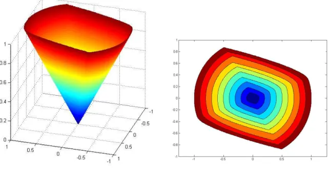
The second example is a two dimensional system which is easily verified to be ISS (hence ISDS) because it is a cascade of two ISS systems. It is given by
˙
x1(t) = −x1(t) + 3x2(t)
˙
x2(t) = −x2(t) + w(t) (6.2)
For γ(r) = 10r and g(r) = r/10 Figure 6.2 (left) shows the lower boundary of the invariance kernel, which in this case happens to be an epigraph, i.e., the figure shows the graph of the ISDS
Lya-punov function which was computed using the functional approximation. Figure 6.2 (right) shows the corresponding level sets.
Figure 6.2: Graph and contour sets for the ISDS Lyapunov function for System (6.2), fW = R
7
Conclusions
The shape of the contour set in our last example suggests that the minimal ISDS Lyapunov function is nonsmooth, indicating that optimal ISDS Lyapunov functions are not in general smooth, a property which is also known for optimal H∞ storage functions, see [10]. Indeed, since the epigraph of the
minimal ISDS Lyapunov function is an invariance kernel and since the invariance kernel is a maximal closed subset (satisfying the invariance property), the minimal ISDS Lyapunov function is necessarily lower semicontinuous but in general it has no reason to be smooth or even continuous. This moti-vates our use of set oriented methods and set–valued analysis, which is an appropriate framework for handling such functions.
References
[1] J.-P. Aubin and A. Cellina. Differential Inclusions. Springer–Verlag, 1984.
[2] P. Cardaliaguet, M. Quincampoix, and P. Saint-Pierre. Set–valued numerical analysis for optimal control and differential games. In Stochastic and differential games, volume 4 of Ann. Internat. Soc. Dynam. Games, pages 177–247. Birkh¨auser, Boston, MA, 1999.
[3] F. Colonius and W. Kliemann. Limits of input–to–state stability. Syst. Control Lett., 49(2):111– 120, 2003.
[4] L. Gr¨une. Asymptotic Behavior of Dynamical and Control Systems under Perturbation and Dis-cretization. Lecture Notes in Mathematics, Vol. 1783. Springer–Verlag, 2002.
[5] L. Gr¨une. Input–to–state dynamical stability and its Lyapunov function characterization. IEEE Trans. Autom. Control, 47:1499–1504, 2002.
[6] L. Gr¨une. Quantitative aspects of the input–to–state stability property. In M. de Queiroz, M. Mal-isoff, and P. Wolenski, editors, Optimal Control, Stabilization, and Nonsmooth Analysis, Lecture Notes in Control and Information Sciences 301, pages 215–230. Springer–Verlag, Heidelberg, 2004. [7] L. Gr¨une, E. D. Sontag, and F. R. Wirth. Asymptotic stability equals exponential stability, and
ISS equals finite energy gain—if you twist your eyes. Syst. Control Lett., 38:127–134, 1999. [8] S. Huang, M.R. James, D. Nesic, and P. M. Dower. Analysis of input to state stability for
discrete–time nonlinear systems via dynamic programming. Preprint, 2002. Submitted.
[9] E. B. Lee and L. Markus. Foundations of Optimal Control. John Wiley & Sons, New York, 1967. [10] L. Rosier and E. D. Sontag. Remarks regarding the gap between continuous, Lipschitz, and differentiable storage functions for dissipation inequalities. Syst. Control Lett., 41:237–249, 2000. [11] P. Saint-Pierre. Approximation of the viability kernel. Appl. Math. Optim., 29:187–209, 1994. [12] E. D. Sontag. Smooth stabilization implies coprime factorization. IEEE Trans. Autom. Control,
34:435–443, 1989.
[13] E. D. Sontag. On the input-to-state stability property. Europ. J. Control, 1:24–36, 1995.
[14] E. D. Sontag. The ISS philosophy as a unifying framework for stability–like behavior. In A. Isidori, F. Lamnabhi-Lagarrigue, and W. Respondek, editors, Nonlinear Control in the Year 2000, Volume 2, Lecture Notes in Control and Information Sciences 259, pages 443–468. NCN, Springer Verlag, London, 2000.
[15] E. D. Sontag and Y. Wang. On characterizations of the input-to-state stability property. Syst. Control Lett., 24:351–359, 1995.
![Figure 4.3: Numerically determined invariance kernel Inv ψ ˜ (D) for System (4.1), f W = [−0.12, 0.12]](https://thumb-eu.123doks.com/thumbv2/123doknet/2610366.57761/12.918.276.625.154.465/figure-numerically-determined-invariance-kernel-inv-ps-d.webp)