Conception of a near-infrared
spectrometer for ground-based
observations of massive stars
Christian Kintziger
Richard Desselle
Jerome Loicq
Gregor Rauw
Pierre Rochus
near-Conception of a near-infrared spectrometer for
ground-based observations of massive stars
Christian Kintziger,a,*Richard Desselle,a Jerome Loicq,aGregor Rauw,band Pierre RochusaaCentre Spatial de Liège, Angleur, Belgium
bUniversité de Liège, Institut d’Astrophysique et de Géophysique, Groupe d’Astrophysique des Hautes Energies, Liège, Belgium
Abstract. In our contribution, we outline the different steps in the design of a fiber-fed spectrographic instrument for stellar astrophysics. Starting from the derivation of theoretical relationships from the scientific requirements and telescope characteristics, the entire optical design of the spectrograph is presented. Specific optical elements, such as a toroidal lens, are introduced to improve the instrument’s efficiency. Then the verification of predicted optical performances is investigated through optical analyses, such as resolution checking. Eventually, the star positioning system onto the central fiber core is explained. © 2017 Society of Photo-Optical Instrumentation Engineers (SPIE) [DOI:10.1117/1.JATIS.3.1.015002]
Keywords: spectroscopy; instrumentation; massive stars; TIGRE telescope; optical design.
Paper 16042P received Aug. 3, 2016; accepted for publication Feb. 1, 2017; published online Feb. 21, 2017.
1
Introduction
1.1 Astrophysical Background
The full understanding of astrophysical sources requires access to a rather wide wavelength range. Every wavelength domain provides another specific piece of information that is needed to solve the puzzle. However, some wavelength domains have been somewhat neglected in recent years despite their enormous potential. This is the case, for instance, of the near-IR domain around 1 to 1.1μm, notwithstanding the fact that this wave-length domain can be accessed from the ground. The main reasons for this situation are the decrease in sensitivity of con-ventional CCD detectors in this region and the fact that most instruments are designed for longer wavelength studies, e.g., to study the J (1.22μm), H (1.63 μm), and K (2.19 μm) bands, which are largely used in photometry.
The near-IR domain around 1μm has an enormous diagnos-tic potential for stellar activity and stellar winds. Stellar winds are prominent features of massive stars, i.e., stars at least 10 times more massive than our Sun. Indeed, these stars are very hot and luminous. Their strong UV radiation fields drive ener-getic and dense stellar winds that have a strong impact on the surrounding interstellar medium. In this context, the wavelength domain near 1μm is particularly interesting as it contains many spectral lines whose profiles provide useful information about stellar winds over almost the entire range of stellar masses. For example, this region contains the He Iλ 10830 line, one of the few unblended He I lines. As it forms over almost the entire stellar wind, it has a huge diagnostic potential for models of stel-lar winds. Its morphology ranges from an absorption line in stars with low density winds to a broad P-Cygni profile in Wolf-Rayet stars.1,2In some cases, the emission part of the P-Cygni profile is flat-topped, in other cases, it is rounded or strongly peaked.3The morphology of the line reflects the velocity law in the wind and can thus provide unique information. Moreover, this line is a
good indicator of variability in the wind,3 especially for the so-called luminous blue variables, which are in an intermediate evolutionary stage between O and Wolf-Rayet stars, where important quantities of material are lost.
Last but not least, phase-resolved observations of the He Iλ 10830 line in massive binary systems are a powerful diagnostic of wind–wind interactions in these binaries.4But He Iλ 10830 is of course not the only interesting line in this spectral domain (see Fig.1). Other features include He IIλ 10124, Pa δ and Pa γ, C III and C IV lines, etc.
On the other hand, this spectral region is also of interest for studies of the activity of low mass stars. In cool M dwarf stars, chromospheric activity is a wide-spread phenomenon which manifests itself through quiescent line emission (Ca II H and K, Hα) in the optical in addition to dramatic flaring events. Recently, it has been shown that emission in the higher order Paschen lines of hydrogen (Pa β, Pa γ, and Pa δ) as well as He Iλ 10830 is a good proxy of a strong flaring activity.5–7Also, in the case of solar-type stars, He Iλ 10830 and the Paschen lines are excellent indicators of chromospheric activity.8
Moreover, this spectral range also provides key information on the circumstellar environment of cool giants. Indeed, in some cool giants such as Arcturus (K2 III), a highly variable He Iλ 10830 emission has been observed and was attributed to shock waves in otherwise elusive chromospheres.9Yet, in other objects, such as HD6833 (G9.5 III), the line was found in absorption, but with a blueward extension that reveals the existence of a stellar wind.10
Finally, the He Iλ10830 line is also of major interest for the study of accretion in classical T Tauri stars. T Tauri stars are low-mass pre-main-sequence stars that are still accreting material from a circumstellar disk. The emission lines observed in the spectra of these stars form at the star-disk interface or in the inner disk region. These regions have a complex topology. The high opacity of He Iλ10830 makes it a sensitive probe of both the accreting matter, in emission, and the outflowing gas *Address all correspondence to: Christian Kintziger, E-mail:ckintziger@ulg.ac.
via the frequently detected absorption features. Observations of this line in T Tauri stars can thus be used to constrain the wind geometry of such accreting objects.11,12
In summary, it is obvious that the spectral region around the He Iλ 10830 line has a huge potential for many topics in stellar astrophysics. Therefore, several research groups from Liège University have joined their forces to develop a spectrograph that covers this wavelength domain with the goal to install it at the TIGRE telescope.
1.2 TIGRE
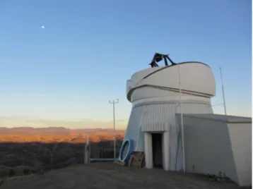
The TIGRE, formerly called Hamburg Robotic Telescope (HRT), is a fully robotic telescope located in La Luz, Mexico13 (see Fig. 2). This private telescope is installed at an altitude of 2400 m on a site operated by the University of Guanajuato. TIGRE is a collaboration between the universities of Hamburg (Germany), Guanajuato (Mexico), and Liège (Belgium).
Currently, the only scientific instrument under operation on the TIGRE is HEROS, a double-channel spectrograph fed with the telescope’s light through an optical fiber. Spectroscopic light in La Luz was first achieved in April 2013 and regular automatic observations from Hamburg started on August 1, 2013.
The TIGRE is anF∕8 Cassegrain telescope, whose primary mirror has a diameter of 1.2 m. The typical seeing at the La Luz site amounts to 2 arc sec on average, approaching 1 arc sec for good nights. Therefore, this telescope is particularly well suited for the spectroscopic study of bright stars. The telescope benefits from a modern Alt-Az mount and concentrates light through a three-mirror assembly to a Nasmyth focus. The spectrographic instrument that we present will be connected to the telescope through a fiber whose entrance will be placed at the currently vacant Nasmyth focus of the TIGRE telescope. The other end of this fiber will feed the instrument located in a separate building neighboring the telescope dome.
1.3 Proposed Near-Infrared Spectrograph
Although those wavelengths can be observed from the ground, the near-infrared region is somewhat neglected due to techno-logical issues, such as the decrease in sensitivity of conventional CCD detectors in that spectral domain. We have designed a near-infrared spectrograph to partially fill the gap in this area. The optical design features a minimum resolution equal to 20,000 within the waveband of interest that ranges from 1 to 1.1μm. A rotating grating enables the scan of smaller waveband regions to cover the entire wavelength domain. On the other hand, wavelength calibration and flat-fielding are performed with the help of internal calibration lamps that can be selected by a translation stage.
The instrument’s interface consists of a fiber bundle that feeds the collimator mirror with stellar light from the telescope. On the other hand, a simultaneous sky background measurement is accomplished through the use of dedicated fibers surrounding the central ones, which are located near the target position within the telescope focal plane. Eventually, the circular bundle input is reshaped into a linear configuration to form the entrance slit of the spectrograph.
The fiber option to connect the spectrograph to the telescope opens up the possibility to also use the instrument at other telescopes in the future. A versatile interface was, therefore, required to enable such capabilities and the choice of using a fiber bundle was made.
Table1summarizes the scientific requirements for the pro-posed spectrograph.
2
Optical Design
2.1 Basic Considerations
The scientific requirements impose the spectrograph resolution power to be at least 10,000, the ultimate goal being 20,000 over the spectral range 1 to 1.1μm. Therefore, the detector must exhibit a minimum of 3810 pixels in order to sample each wave-length resolution element with at least two pixels and to cover the entire waveband of 100 nm at the highest resolution power. Since typical near-infrared detectors incorporate pixels that are 30μm wide, the results show that the required detector size is approximately equal to 12 cm and that the number of pixels exceeds the typical available detector sizes which are lim-ited to approximately a thousand pixels. The direct consequence is that the total waveband of interest may not be covered in a single exposure unless an echelle spectrograph is considered. In our case, the imaging direction is used for sky background measurements as well as other potential targets falling onto
Fig. 1 Observation of the near-IR spectrum of the Wolf-Rayet star WR1362 recorded with a CCD detector. The absorption features
between 8900 Å and 1 μm are due to the Earth’s atmosphere.
(Figure courtesy Jean-Marie Vreux).
the bundle, therefore, the solution consisting of using a cross-disperser is currently not foreseen.
The reciprocal dispersion or plate factor may also be evaluated in first approximation. Considering the goal wavelength resolu-tion element and the typical pixel size of near-infrared detectors, the required reciprocal dispersion rises to 0.875 nm∕mm.
In Sec.2.2, we perform further calculations to convert the scientific requirements into instrumental requirements. 2.2 From Scientific Requirements to Technical
Ones
The first choice before starting any optical design or parameter calculation is to decide upon the nature of the dispersive element used inside the spectrograph, i.e., whether using a diffraction grating or a prism. According to Jacquinot analyses, gratings outperform similar size prisms by a factor of 50 to 100 in the near-infrared,15thus a grating is selected. A Czerny–Turner con-figuration is adopted from several options that exist. One of its advantages is the coplanarity between entrance and exit slits that is enabled through the separation of the collimating and focus-ing functions of the instrument. On the other hand, more degrees of freedom are made available to the designer due to the addi-tional mirror element, which helps to tackle the optical aberra-tions.16Moreover, the ability to cover a wide spectral range by, for example, rotating the grating makes it a suitable candidate to record the spectrum of the entire required waveband.17 Event-ually, several studies identified techniques to deal with the inher-ent aberrations of this design.
When starting the conception of a new instrument from scratch, the first step is to translate the scientific requirements into technical specifications. This means obtaining rough esti-mates or relations between parameters involved in the optical design of a spectrometer. The complexity of this problem stems from the fact that several parameters appear when considering a whole spectrograph. Bingham identified 16 parameters for a grating spectrograph combined with a telescope and proposed a systematic approach to calculate them.18The method concerns plane reflection gratings but can be adapted to curved ones. Those parameters are listed in Table2.
Bingham’s method consists of maximizing figures of merit and fixing some basic parameters to obtain all the others in such
a way that the derived instrument satisfies the scientific require-ments properly. The relations used to derive the entire set of parameters are seven basic equations describing a standard reflection spectrograph (see Ref.18for details).
Since 16 parameters are identified, 9 variables are sufficient to describe a whole spectrometer. These are the telescope diam-eterAtel and its focal lengthftel (which are fixed for a given
telescope), the grating orderm and the central wavelength λ, as well as five free parameters of Bingham’s “spectrometer-like” method, which areR, θs,w0,α þ β, and α − β.
This technique18is employed here to obtain a first glance onto the spectrograph’s parameters. The scientific requirements paired to the telescope’s characteristics as well as off-the-shelf gratings availability enable the definition of six of the nine parameters. Indeed, the telescope focal length and its diameter are specified in Sec.1.2, while Table1specifies a goal resolu-tion of 20,000 and a central wavelength of 1050 nm. On the other hand, a commercially off-the-shelf first order (m ¼ 1) gra-ting with a blaze angle (ðα þ βÞ∕2) of 41.3 deg, the maximum one found around 1μm to follow Bingham’s advice is consid-ered here.
The entrance slit angular size of the spectrograph may be matched to the maximum seeing of the telescope site. This way, the entire light beam from the target star will enter the con-nected spectrograph instrument. On the other hand, the spatial extent of the entrance slit is nothing else than the diameter of the fiber optic core, which links the telescope to the spectrograph. Considering a maximum seeing of 2 arc sec,θs may be given
Table 1 Scientific requirements for the proposed near-infrared spectrograph.
Parameter Requirement Goal
Spectral range 1000 to 1100 nm 940 to 1400 nm Resolving power 10,000 20,000 Target magnitudes V < 7 V < 9 Signal-to-noise ratio in continuum 100 at V ¼ 6 100 at V ¼ 7
Typical exposure time 15 to 30 min 15 min
Simultaneous sky measurements Yes Yes Wavelength calibration accuracy δλ∕20 ¼ 0.05 Å δλ∕20 ¼ 0.025 Å
Table 2 Parameters involved in the description of a spectroscopic instrument.
Symbol Parameter
R Resolving power
D Dispersion [mm∕nm or mm∕Å]
θs Angular entrance slit size
α þ β Sum of incidence and diffraction angles on grating
α − β Difference between incidence and diffraction
angles on grating
m Grating order
Atel Diameter of the telescope’s primary mirror
ftel Focal length of telescope
Acoll Collimator size
fcoll Focal length of collimator
Acam Focuser/camera size
fcam Focal length of focuser/camera
L Grating size (across grooves)
w0 Exit slit size
λ Wavelength
this value in a first approach. However, the manufacturing capa-bilities of the selected grating specify a limited size of 154 mm, thus the entrance slit maximum spatial extent rises to 80.82μm. The availability of optical fibers now restrains the possibility of using this width for the entrance slit of the spectrograph. Commercially available multimode fibers are mostly available with core diameters ranging from 25 to hundreds of microns, varying in size by a factor of 2. No suitable commercial off-the-shelf 80-μm core fiber could be found. Since the manufac-turing of a custom one is definitely an expensive option, the selection of a 50-μm core standard fiber is, therefore, a reason-able starting point for an iteration of Bingham’s method.
The use of such a thinner optical fiber than required leads to flux losses at the fiber entrance for typical seeing conditions at La Luz observatory, though the HEROS spectrograph currently under operation at the TIGRE telescope employs a 50-μm core fiber optic associated with microlenses engraved at both ends within its own material.13This way, the average star image of approximately a hundred microns under a typical 2 arc sec see-ing entirely falls into the 50-μm fiber core. Moreover, this also adapts the focal ratio of the telescope to that of the fiber in order to minimize the induced focal ratio degradation (FRD). This sol-ution is also foreseen for the proposed spectrograph to avoid large light losses at the fiber entrance. Moreover, the microlens located at the spectrometer side of the fiber contributes to reshaping the light beam back to its initialF# of 8. The induced change in spatial extent due to conservation of etendue through the exit microlens will, however, decrease the resolving power of the instrument.
In the meantime, the photometric performance of the instru-ment is assessed in Fig.3. For that purpose, FRD properties of fibers studied by Carrasco and Parry19and Barden20are used to investigate the required integration time to reach the SNR speci-fied in Table1. Their data on both poor and high quality fibers are employed. Moreover, typical and nice seeing conditions are simulated and the use of microlenses is also examined. Figure3
introduces the obtained results when simulating the observation under typical seeing conditions: Fig.3(a)[respectively (b)] high-lights the fact that an upper limit of 5.5 (respectively 5.8) on the star magnitude in J-band arises when using a poor (respectively
high) quality fiber. When the seeing approaches 1 arc sec on good nights, this limit disappears and the maximum integration time falls to 8 min for poor quality fibers. Eventually, the use of microlenses decreases this observation time to 3 min. The 30-min limit specified in Table1may, therefore, only be fulfilled during good nights and a slightly lower star magnitude consid-ered otherwise until microlenses are installed.
When considering the choice of a suitable sensor, we note that near-infrared detectors are commonly used are InGaAs or HgCdTe sensors rather than CCD matrices due to their lack of performance in that region of the spectrum. Their pixel pitch usually ranges from 15 to 30μm with a majority exhibiting the latter. Therefore, w0 is given a value of 60μm as a first approximation.
The last parameter to be fixed to initiate the spectrometer-like method is α − β. This angle can be associated with the one formed by the collimator-grating-camera sequence of the optical elements. The effect of this angle on the inferred parameters has been deeply investigated by Bingham.18Following the analyses of Allemand,21 illuminating the grating in a given range of angles, between 0.6 and 0.9 rad, leads to a reduction of the coma aberration through the focal field of Czerny–Turner spec-trographs (see Allemand21for exact assumptions and approxi-mations). As a starting point, the grating incident angle is then fixed toα ¼ 35 deg and therefore α − β is equal to −12.6 deg. The results of an iteration of the spectrometer-like method are shown in Table3. The first nine parameters are fixed through the above considerations, whereas the last seven are deduced. The obtained spectrograph’s specification constitutes a basic starting point for optimization with optical design software and is subject to changes when considering, for example, aberrations and further optical analyses such as resolution calculations. 2.3 Optimization Process
Once the first technical specifications of the spectrograph are known, the optimization process can start in order to obtain the required imaging capabilities. These operations are performed with CODE V optical design software.22
Starting from the previously obtained values for the spectro-graph’s specifications, the optimization is performed by varying
Fig. 3 Required integration time to reach a SNR of 100 when considering (a) poor quality fibers and (b) high quality ones. Several star effective temperatures are considered.
the locations of the different optical elements as well to obtain an ideal matching between optical elements’ positioning and manufacturing.
Different approaches may be followed in order to guide the optimization process and obtain a rough location of the optical elements as a starting point. Many studies are available to optimize Czerny–Turner spectrographs, mostly focused on tech-niques to face the astigmatism of such designs. They elaborate suitable guidelines concerning the use of specific elements to incorporate into the design to tackle the inherent aberrations of Czerny–Turner spectrographs. Specific positioning of optical components is also advised to meet conditions that minimize the
effects of aberrations that play a major role in the overall optical quality of the instrument.
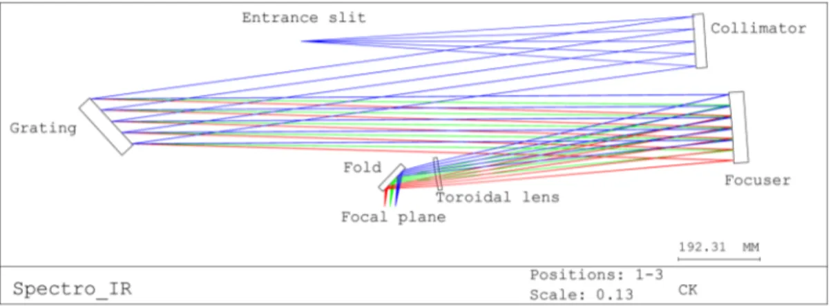
The use of cylindrical and toroidal optical elements in Czerny–Turner spectrographs is explored by some authors to counter the astigmatic behavior of those instruments. For exam-ple, Xue et al.23propose using a toroidal focusing mirror instead of a spherical one to control both sagittal and tangential focal lengths separately and decrease the astigmatism. Moreover, they find an adequate distance between the grating and the focusing mirror so that the aberrations are balanced over a wide spectral range. They eventually recall mathematical con-ditions to limit other aberrations, such as the spherical and coma ones, the latter being known as the“Shafer equation.”24Xue also suggests another possibility that consists of incorporating a wedged cylindrical lens into a Czerny–Turner spectrograph to achieve an astigmatism correction for broadband spectral simultaneity.25Another solution, geometrical this time, is pro-posed by Austin et al.26to avoid astigmatic blurring effects: using divergent illumination of the grating instead of collimating light and an adapted positioning to obtain broadband perfor-mances. Eventually, a cylindrical lens is used by Lee et al.27 to correct for astigmatism over a wide spectral range with the help of low-cost optics. The general methodology remains the same: incorporating into the design an asymmetry in order to be able to decrease the inherent astigmatism in such spectrometers. The implemented method for the proposed spectrograph uses a toroidal lens that is located close to the focal plane. The differ-ence between its tangential and sagittal focal lengths produces the required asymmetric parameter that enables the correction of astigmatism. A similar philosophy to Lee et al.’s methodology is followed in order to use smaller size low-cost optics. The asym-metric element is, therefore, placed near the focal plane where the converging beam is narrower. Indeed, this avoids the use of a large toroidal focusing mirror. Figure 4 illustrates the optical design, where the typical collimator-grating-focuser optical chain is represented. The toroidal lens and a folding mirror are inserted close to the focal plane located at the bottom of Fig.4. The fold-ing mirror utility consists of deliverfold-ing some room for the detector and avoiding any interference with the optical beam.
2.4 Resolution Analysis
The optimization process consists of improving the quality of spots, i.e., images of point sources located at different places through the entrance slit. As the exit slit blurs, it gets away from the required ideal size and the resolving power decreases.
Table 3 Spectrograph’s parameters obtained when running
Bingham’s method. Parameter Value Atel 1.2 m ftel 9.6 m m 1 λ 1050 nm R 20 000 θs 1.074 arc sec w0 60 μm α þ β 41.3° α − β −12.6° fcoll 624.339 mm Acoll 78.042 mm fcam 616.725 mm Acam 64.242 mm 1∕d 1249.554 lp∕mm L 95.272 mm D 0.875 nm∕mm
The optimization process was, therefore, naturally driven by an evaluation of the resolution through the focal plane involving spot sizes.
The developed methodology to evaluate the resolution through the instrument focal plane during optimization consists of the calculation of the sampled waveband of each pixel. The entire bidirectional focal plane is scanned, which means probing the resolution changes with wavelength along the spectral direc-tion, and through the slit along the imaging direction.
The waveband that each pixel samples is obtained by com-puting the evolution of the inscribed area of the slit width into this pixel as the wavelength varies. The limiting footprint of the exit slit is approximated by the distance between the edges of the spots from points located at opposite sides of the entrance slit. This criterion considers 100% of the energy as uniformly dis-tributed all over the spot and thus does not take into account the typical Gaussian profile of a point spread function. The evaluated exit slit width through this method is, therefore, slightly pessimistic since it tends to first enlarge its width and, on the other hand, consider its profile as a uniformly dis-tributed rectangular function. Figure5(a)illustrates a step of the spectral profile calculation at 1040 nm, where the local pixel is
represented by a black rectangle. Figure 6(a) depicts the obtained profile at a given wavelength and position through the entrance slit.
The obtained triangular-shaped profile of one pixel’s sampled waveband is nothing else than the convolution of two rectangular functions, which are the pixel window and the approximated exit slit width [see Fig.6(a)]. The local resolution power is then evaluated as the ratio between the central wave-length and the full width at half maximum (FWHM) of the spec-tral profile. The result of this analysis is a map of the resolution power as a function of the local wavelength and the vertical posi-tion of the slit, i.e., the selected fiber [see Fig.6(b)for a selected grating position].
A symmetric variation of the resolution power with respect to the slit center can be observed due to changes in spot sizes. This deviation also occurs with respect to wavelength as the spots actually differ in shape rather than size. Indeed, since 100% of the spot is considered regardless of its actual energy distri-bution, a slight change in shape with no impact on its RMS size leads to a variation in resolution with the employed methodol-ogy. This behavior can be observed in Figs.5(a)–5(c), where the spots are depicted at different wavelengths. Therefore, the 100%
Fig. 5 Plot of exit slit spots from points located at the sides (red and blue) and center (green) of the entrance slit. The slit is elongated along the horizontal direction. The situation is depicted at three different wavelengths that are (a) 1040 nm, (b) 1050 nm, (c) and 1060 nm.
Fig. 6 (a) Plot of one sampled exit slit profile and (b) resolution power across focal plane for a given grating position.
spot size does not suit accurate resolution calculation but rather allows assessing it in a first approximation. An exit slit profile taking into account the energy distribution must be considered to obtain more accurate results.
The second resolution analysis that is developed in ASAP optical software28consists of illuminating the overall entrance slit, considered as a rectangle of 50μm × 10 mm, and observing its image at the focal plane of the instrument. By doing so, the exact slit profile can be examined and used to calculate the resolution power in a proper way.
In order to investigate the evolution of the resolution power through the entire focal plane, the exit slit profile is observed at several wavelengths and multiple places along the imaging direction. In contrast with the previous method, the energy dis-tribution over the exit slit is computed and used to evaluate the resolution power. A polynomial fitting is eventually performed to calculate the dispersion relation, which associates each pixel of the focal plane with a specific wavelength. The FWHM of the exit slit spectral profile can then be evaluated and the corre-sponding resolving power is calculated. Figure 7(a)illustrates the sampling of the exit slit at a given height and wavelength. The obtained results produce an updated bidimensional map-ping of the resolution power, whose two directions are the wave-length and the position through the exit slit [see Fig.7(b)].
The values obtained are, as expected, higher than those found with the previous method since the uniform rectangular shape approximation is abandoned. The slit blurring due to changes in spot sizes is the only cause here for resolution degradation and the deformation of the spots does not impact the results anymore. As a consequence, the previously observed change in resolution with wavelength disappears. Indeed, the measured variation in this case amounts to ∼2%, whereas the previous change was 10%. The slight slope in resolution with wavelength is due here to the change in considered local wavelength in the calculation ofλ∕δλ.
In conclusion, the optimization process driving criterion underestimated the resolving power, which amounts to an aver-age value of∼29;000. The obtained design, therefore, overfills
the scientific requirements by 45%, but the performed analyses neglect any alignment or manufacturing error. The final resolv-ing power actually reached will then be lower and a tolerancresolv-ing analysis is required to investigate the induced variation.
It is interesting to run Bingham’s spectrometer-like method one more time to get the spectrometer specifications that are obtained when starting with the same basic parameters from Table3except for the resolution that is now fixed to 29,000. These are compared to the spectrometer parameters reached when following the pessimistic resolution criterion in Table4
(only the seven deduced ones are listed). A fine matching between both methods appears, confirming the validity of Bingham’s spectrometer like methodology.
2.5 Straylight Analysis
The straylight analysis intends to identify and mitigate potential unwanted paths of light reaching the detector that may cause blurred images or decrease the signal-to-noise ratio, for exam-ple. The interaction between the optical design and its surround-ing instrument walls is considered here to account for any multiple reflection paths. Eventually, this analysis leads to the design of suitable internal panels that aim at blocking these straylight sources.
Particular care is given to the out-of-band wavelengths, i.e., the ones that vignette and reach the detector after a few reflec-tions onto the instrument walls. Their propagation through the system is stopped with the help of a specific enclosure around the detector, which selects the waveband of interest.
Direct paths from the calibration lamps are also prohibited and an accurate shielding is required to cope with the wide open-ing angle of the cone of light emitted through the entrance slits. On the other hand, the zeroth diffraction order from the grating may also lead to problems. In our design, the rays from this pol-ychromatic straylight source follow trajectories that impact the left side of the calibration unit, where an internal panel is added to form a light trap (see Fig.8).
Fig. 7 (a) Plot of one sampled exit slit profile and (b) resolution power across focal plane for a given grating position.
The ghost generated from the toroidal lens imperfect trans-missivity is also studied. This second order ghost image is formed between the folding mirror and the toroidal lens. Considering that an antireflective coating is applied on both sides of the lens, only a negligible pale veil spreads over the detector due to the internal reflections that occur through the lens.
Those considerations lead to the instrument mechanical enclosure that is shown in Fig.8.
3
Calibration
3.1 Spectral Calibration
The calibration of the instrument requires a repeatable source featuring precise spectral lines in order to attribute to each pixel of the detector the correct wavelength.
Typical lamps used for this calibration purpose are hollow cathode lamps (HCL). HCL commonly used for astronomical applications incorporate a buffer gas consisting of several atomic species. Typical mixtures involve Thorium and Argon gases for the calibration of spectrographs operating from the vis-ible to the infrared part of the spectrum. For example, an atlas reporting more than 2400 lines of a Th-Ar HCL is available for
the wavelength calibration of the Cryogenic High-Resolution IR Echelle Spectrometer (CRIRES) at the very large telescope.29 Another atlas that covers the near-infrared spectrum from 1798 to 9180 cm−1(i.e., from 1089 to 5561 nm) is provided by Engleman et al.30 Other mixes of gases are also used, such as uranium–neon when calibrating spectroscopic instruments in the near-infrared. Feasibility studies about using lamps, which incorporate uranium as the primary source in spectro-scopic applications, were realized as early as in the late 1960s.31 Atlases reporting spectral lines obtained with such HCL exist32,33and are used as calibration sources for astronomical spectroscopy purposes.34
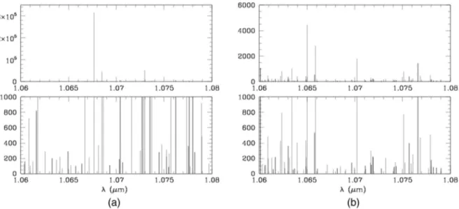
The choice of using a U-Ne HCL was made in order to cal-ibrate our spectrograph. The selection between a Th-Ar or U-Ne HCL is motivated by the number of high intensity lines in the 1.0 to 1.1μm waveband. When looking at Fig. 9, where the spectra from a Th-Ar [Fig. 9(a)29] and a U-Ne [Fig. 9(b)32] HCL are plotted, it can be observed that very strong lines appear in the Th-Ar spectrum between 1060 and 1080 nm, for example. These lines completely outshine many fainter ones whose inten-sities are much lower, as can be seen when zooming onto the lower part of the intensity axis [see Fig.9(a)bottom]. This sit-uation will likely lead to saturation of the detector for the strong-est lines, while leaving the weaker ones badly underexposed. On the other hand, Fig.9(b)reveals the same part of the spectrum as produced by a U-Ne lamp. Though some strong lines are still present, their relative intensities compared to the weaker lines are much less extreme compared to the Th-Ar lamp.
3.2 Flat-Field Calibration
Flatfield calibration consists of correcting astronomical images for the pixel to pixel variation in sensitivity. Illuminating the spectrograph with a known continuum source enables measur-ing those fluctuations.
The required lamp to perform such a calibration must, there-fore, exhibit a continuous spectrum over the considered wave-band of interest, i.e., from 1 to 1.1μm. Typical halogen lamps are used to flat-field near-infrared spectrographs as is the case for the K-band multifield spectrograph currently installed at the VLT.35A halogen lamp is selected as a flat-field calibrator for the proposed spectrograph instrument.
3.3 Practical Implementation
The calibration unit of the instrument is located near the optic fiber entrance and features two illuminated mechanical entrance slits positioned at symmetrical places with respect to a moving fold mirror (see Fig.10). The folded path of light connects the output end of the fiber to the collimator when the mirror stands in its down position. When calibrating, the moving mirror moves upward and the light from the calibration box illuminates the collimator. A beamsplitter is used to collect the light from both lamps and inject it onto the collimating mirror.
To move the folding mirror in and out of the calibration light beam, we first considered a flipping mechanism. The mechani-cal repeatability of this component is, however, not sufficient to achieve the calibration accuracy needed to fulfill the scientific requirements (see Table1). Indeed, a rough repositioning of the mirror after calibration induces a shift in wavelength measure-ment that must be avoided for precise calibration of stellar spec-tra. The comparison of the two components is represented in Fig.11.
Fig. 8 Propagation of the rays from the zeroth diffraction order of the grating. Light is confined at the top left after hitting the walls of the calibration unit compartment and does not reach the detector. Table 4 Comparison between spectrometer specifications obtained with both first resolution criterion and Bingham’s spectrometer method to achieve a resolving power of 29,000.
First resolution criterion Bingham’s spectrometer method
Parameter Value Parameter Value
fcoll 938.136 mm fcoll 905.291 mm Acoll 120 mm Acoll 113.161 mm fcam 888.395 mm fcam 894.251 mm Acam 100 mm Acam 93.151 mm 1∕d 1200 lp∕mm 1∕d 1249.554 lp∕mm L 150 mm L 138.145 mm D 0.79 nm∕mm D 0.603 nm∕mm
Light is first injected through the fiber channel when the moving mirror is settled within its maximum positioning error. Calibration is then performed through the HCL path and the detected wavelength is measured along the entire slit length with the help of the polynomial dispersion relation. The measured wavelength profile over the exit slit height is altered since the HCL and fiber channels are not perfectly superposed. Typically, the entire profile shifts vertically, which induces a wavelength off-set in measurements. Figure11(a)[respectively (b)] illustrates the simulation results when taking into account the accuracy of the flipping mechanism (respectively the translation stage).
The calibration precision specified in the scientific require-ments states a value ofδλ∕20. Figure11(a)immediately proves
that the mechanical repeatability of the flipping component cannot reach such a precision. Indeed, the measured shift in wavelength rises to 2.25 times the requirement, thus the mean detected wavelength does not fall inside the acceptance zone defined by the two horizontal dashed green lines. On the other hand, the translation stage precision leads to a wave-length error of 0.1 times the specified maximum value and the mean detected wavelength, represented by a red line, is located in the tolerated error interval [see Fig.11(b)].
4
Star Positioning System
4.1 Purpose of the Instrument
When collecting the light from a telescope and feeding a spectrographic instrument with the help of a fiber, a perfect alignment of the star image with the fiber core must be achieved in order to maximize the transmitted flux to the instrument. A system must then be developed in order to be able to drive the telescope pointing and align the target image with the fiber core. To do so, both the star and the fiber core images may be visu-alized on a single camera and the alignment process consists of bringing them close together until they superpose.
4.2 Optical Design
The proposed system is made of a beamsplitter, a spherical mir-ror, and a guiding camera (see Fig.12). Moreover, a backillu-minating system of the fiber is included into the spectrometer housing. This way, the fiber can be lit by its spectrograph-side output and inject light toward the telescope. To do so, an LED can be turned on and imaged onto the fiber with the help of an achromatic doublet inside the spectrograph when the fold mirror stands in its up position. The translation stage is, therefore, used for both calibration and star positioning processes.
The selected beam-splitting optical element is an off-the-shelf antireflective window to be used in the near-infrared wave-band. This exotic choice intends to minimize the proportion of useful light, i.e., belonging to the 1- to 1.1-μm waveband that is used for star positioning to the detriment of stellar spectra
Fig. 9 (a) Th-Ar spectrum29between 1060 and 1080 nm and (b) same part of the spectrum obtained from
a U-Ne lamp.32Bottom parts of both figures are zooms from upper ones obtained when limiting the
intensity y-axis.
Fig. 10 Calibration unit optical design. Light coming from the output end of the fiber reaches a moving fold mirror when positioned in its down position and is injected to the collimating mirror during obser-vation (right to the fold mirror, not represented in the figure). When calibrating, the moving mirror moves upward and light from the cali-bration lamps is gathered with a beamsplitter and eventually goes to the collimator.
recording. Indeed, the antireflective coating of the window works fine for near-infrared wavelengths, but quickly loses those characteristics when considering visible light. This part of the spectrum is thus prevented from propagating into the spectrograph and used for guiding purposes. Moreover, this also serves as a first“visible filter” since less luminous visible straylight pollutes the spectrograph.
Due to atmospheric refraction, the near-infrared and the vis-ible images of a star may not overlap exactly. This effect will have to be calibrated during the commissioning phase of the instrument. This problem affects all ground-based observatories and is usually tackled with an atmospheric dispersion compen-sator. Such an instrument is foreseen as a future upgrade to the
spectrograph under development and will be incorporated into the SPS at the telescope focus. The aberration study of such prisms in a converging beam is studied by Wynne and Worswick.36
In the meantime, the aligning strategy will focus on a short waveband centered at 889 nm due to a narrowband methane fil-ter. The differential refraction between the reference targeting and scientific wavelengths of interest can be evaluated with the help of atmospheric dispersion models. According to Szokoly, the most up-to-date atmospheric determination formula belongs to Ciddor calculations and these are used hereafter.37,38 The maximum differential refraction observed at 1.1μm for a zenith distance of 60 deg when aligning at 889 nm amounts to 0.19 arc sec. The near-infrared star image then lies at a maximum dis-tance of 9μm away from the fiber center. Eventually, the inte-gration time required to achieve a signal-to-noise ratio of 100 is estimated to a few seconds considering the entire SPS optical chain efficiency and the filter waveband.
Once the information about the star position is known, the fiber location has to be determined in order to coalign both. This is the utility of the LED located inside the spectrograph housing which illuminates the fiber. This way, visible light is transmitted to the telescope and reaches the antireflective win-dow. This reflected light path is then focused with the help of a spherical mirror through the window onto the camera. The fiber is now imaged onto the camera and the star-to-fiber matching can be performed.
5
Conclusion
A spectrograph instrument was designed to meet the scientific requirements summarized in Table1. Their translation into tech-nical requirements initiated the optimization process that incor-porated a toroidal lens. The purpose of this optical element was to tackle the main aberration of Czerny–Turner spectrographs: astigmatism. The performed photometric budget shows that a slightly lower star magnitude should be observed to fulfill the
Fig. 11 Detected wavelength along the slit length when taking into account the error on the repeatability of (a) the flipping mechanism and (b) of the translation stage. The horizontal red line represents the mean detected wavelength and the two dashed green ones are located at plus and minus the calibrating requirement from the exact injected wavelength.
Fig. 12 Star positioning system. The instrument intends to align the observed target image with the fiber core to maximize the transmitted flux from the telescope to the spectrograph.
requirement on integration time until microlenses are installed for proper fiber coupling with the telescope. The resolution driving criterion and fine analysis were then presented. The optical studies also included a straylight analysis, which led to the design of the instrument mechanical enclosure and internal walls.
Other complementary units were eventually designed to pro-vide the instrument with calibration and telescope guiding abil-ities. On the one hand, specific lamps were identified to perform both spectral and flat-field calibrations. On the other hand, the star positioning system is an instrument complement, which was developed to locate the target image onto the fiber bundle entrance. This way, as much light as possible is transmitted from the telescope to the spectrograph for spectra recording.
As a future task, assembling and tests of the instrument will assess the validity of the previous analyses.
Acknowledgments
This research was funded through an ARC grant for Concerted Research Actions, financed by the French Community of Belgium (Wallonia-Brussels Federation).
References
1. J. M. Vreux and Y. Andrillat,“O stars He II and H lines in the 1 μ region,” Astron. Astrophys. 75, 93–96 (1979).
2. J.-M. Vreux, Y. Andrillat, and E. Biémont,“Near-infrared observations of galactic northern Wolf Rayet stars,” Astron. Astrophys. 238, 207–220 (1990).
3. J. H. Groh, A. Damineli, and F. Jablonski,“Spectral atlas of massive stars around He I 10830 Å,”Astron. Astrophys.465, 993–1002 (2007). 4. I. R. Stevens and I. D. Howarth,“Infrared line-profile variability in Wolf–Rayet binary systems,”Mon. Not. R. Astron. Soc.302, 549–560 (1999).
5. C. I. Short and J. G. Doyle,“Pa-beta as a chromospheric diagnostic in M dwarfs,” Astron. Astrophys. 331, L5–L8 (1998).
6. C. Liefke, A. Reiners, and J. H. M. M. Schmitt,“Magnetic field var-iations and a giant flare multiwavelength observations of CN Leo,” Mem. Soc. Astron. Ital. 78, 258–260 (2007).
7. S. J. Schmidt et al.,“The first detection of time-variable infrared line emission during M dwarf flares,” in American Astronomical Society, AAS Meeting, Vol. 43, 21832604 (2011).
8. D. Choudhary, U. Tejomoortula, and M. J. Penn,“Dynamics of quiet solar chromosphere at the limb,” in American Geophysical Union Fall Meeting, SH23A-1622 (2008).
9. M. Cuntz and D. G. Luttermoser,“Stochastic shock waves as a candi-date mechanism for the formation of the He I 10830-A line in cool giant stars,”Astrophys. J.353, L39–L43 (1990).
10. A. K. Dupree, D. D. Sasselov, and J. B. Lester,“Discovery of a fast wind from a field population II giant star,” Astrophys. J. 387, L85–L88 (1992).
11. J. Kwan, S. Edwards, and W. Fischer,“Modeling T Tauri winds from He Iλ10830 profiles,”Astrophys. J.657, 897–915 (2007).
12. L. Podio, P. J. V. Garcia, and F. Bacciotti,“He I λ 10830 line: a probe of the accretion/ejection activity in RU Lupi,” Mem. Soc. Astron. Ital. 78, 693–694 (2007).
13. J. H. M. M. Schmitt et al.,“TIGRE: a new robotic spectroscopy tele-scope at Guanajuato, Mexico,”Astron. Nachr.335(8), 787–796 (2014). 14. A. Hempelmann,“TIGRE telescope–general information,” Universität Hamburg, 2013,http://www.hs.uni-hamburg.de/EN/Ins/HRT/hrt_general_ info.html(11 May 2016).
15. J. Hearnshaw, Astronomical Spectrographs and Their History, p. 60, Cambridge University Press, Cambridge (2009).
16. M. W. McDowell, “Design of Czerny-Turner spectrographs using divergent grating illumination,”Opt. Acta: Int. J. Opt.22(5), 473–475 (1975).
17. R. E. Bell,“Exploiting a transmission grating spectrometer,”Rev. Sci. Instrum.75(10), 4158–4161 (2004).
18. R. G. Bingham,“Grating spectrometers and spectrographs re-exam-ined,” Q. J. R. Astron. Soc. 20, 395–421 (1979).
19. E. Carrasco and I. R. Parry,“A method for determining the focal ratio degradation of optical fibres for astronomy,”Mon. Not. R. Astron. Soc. 271(1), 1–12 (1994).
20. S. C. Barden,“Fiber optics at Kitt Peak National Observatory,” in Instrumentation for Ground-Based Optical Astronomy, pp. 250–255, Springer, New York (1988).
21. C. D. Allemand,“Coma correction in Czerny-Turner spectrographs,” J. Opt. Soc. Am.58(2), 159–163 (1968).
22. “Application-Specific Optical Design,” 2016,https://optics.synopsys. com/codev/pdfs/ApplicationSpecificDesign.pdf(13 July 2013). 23. Q. Xue, S. Wang, and F. Lu“Aberration-corrected Czerny-Turner
im-aging spectrometer with a wide spectral region,”Appl. Opt.48, 11–16 (2009).
24. A. B. Shafer, L. R. Megill, and L. Droppleman,“Optimization of the Czerny-Turner spectrometer,”J. Opt. Soc. Am.54, 879–887 (1964). 25. Q. Xue,“Astigmatism-corrected Czerny-Turner imaging spectrometer
for broadband spectral simultaneity,” Appl. Opt.50(10), 1338–1344 (2011).
26. D. R. Austin, T. Witting, and I. A. Walmsley,“Broadband astigmatism-free Czerny-Turner imaging spectrometer using spherical mirrors,” Appl. Opt.48(19), 3846–3853 (2009).
27. K. S. Lee, K. P. Thompson, and J. P. Rolland,“Broadband astigmatism-corrected Czerny-Turner spectrometer,”Opt. Express18, 23378–23384 (2010).
28. “ASAP Reference Guide (2014),” http://www.breault.com/knowledge-base/asap-reference-guide-2014(15 August 2014).
29. F. Kerber, G. Nave, and C. J. Sansonetti,“The spectrum of Th-Ar hol-low cathode lamps in the 691–5804 nm region: establishing wavelength standards for the calibration of infrared spectrographs,”Astrophys. J., Suppl. Ser.178(2), 374–381 (2008).
30. R. Engleman, Jr., K. H. Hinkle, and L. Wallace,“The near-infrared spec-trum of a Th/Ar hollow cathode lamp,”J. Quant. Spectrosc. Radiat. Transfer78(1), 1–30 (2003).
31. G. Rossi and N. Omenetto,“Feasibility of using a uranium hollow cathode lamp as primary source in atomic absorption spectroscopy,” European Atomic Energy Community, Ispra, Italy, Joint Nuclear Research Center, No. EUR—3558. e (1967).
32. S. L. Redman et al.,“The infrared spectrum of uranium hollow cathode lamps from 850 nm to 4000 nm: wavenumbers and line identifications from Fourier transform spectra,”Astrophys. J., Suppl. Ser.195(2), 24 (2011).
33. S. L. Redman et al.,“A high-resolution atlas of uranium-neon in the h band,”Astrophys. J., Suppl. Ser.199(1), 2 (2012).
34. L. F. Sarmiento et al.,“Characterizing U-Ne hollow cathode lamps at near-IR wavelengths for the CARMENES survey,”Proc. SPIE9147, 914754 (2014).
35. S. K. Ramsay et al.,“Calibration of the KMOS multi-field imaging spectrometer,” in Proc. 2007 ESO Instrument Calibration Workshop, pp. 319–324 (2008).
36. C. G. Wynne and S. P. Worswick,“Atmospheric dispersion correctors at the Cassegrain focus,” Mon. Not. R. Astron. Soc. 220, 657–670 (1986).
37. G. P. Szokoly,“Optimal slit orientation for long multiobject spectro-scopic exposures,”Astron. Astrophys.443(2), 703–707 (2005). 38. P. E. Ciddor,“Refractive index of air: new equations for the visible and
near infrared,”Appl. Opt.35(9), 1566–1573 (1996).
Christian Kintziger is a PhD student at the Faculty of Applied Sciences of the University of Liège. He received his BS degree in civil engineering and his MS degree in physical engineering from the University of Liège in 2011 and 2013, respectively. He is currently performing his PhD at the Centre Spatial de Liège (CSL) with the goal of developing new instruments to study massive stars. His current research interests focus on spectroscopic instruments. He is a member of SPIE.
Richard Desselle received his master’s degree in physical engineer-ing from the University of Liège in 2013. He is currently doengineer-ing PhD research at the Centre Spatial de Liège in the field of space instru-mentation onboard small satellites for scientific observation of mas-sive stars in the UV domain. He is a member of SPIE.
Jerome Loicq is an associate professor of the University of Liege. He is teaching spectroscopy in astrophysics and space experiment con-ception. He has more than 15 years of experience in space instrument engineering, optical design, integration, and calibration gained mainly through his participation in ESA and NASA programs. He also has developed an expertise in diffractive optics and photonics to be applied to energy conversion and cataract surgery.
Gregor Rauw is a professor for astrophysics at the Astrophysics & Geophysics Department of the University of Liege. He obtained his PhD from Liege University in 1997. He is first author of 40 articles
in refereed journals and has coauthored another 120 refereed papers. His main research field deals with optical and x-ray spectroscopy of massive stars and their surroundings.
Pierre Rochus is a professor at the University of Liège in space instrument design. He received his MS degree in engineering from the University of Liège in 1974 and his PhD in nuclear physics from the University of Liège in 1979. He is the author of more than 100 journal papers and has written two book chapters. His current research interests include space optical instruments and optoelec-tronic systems. He is a member of SPIE.