O
pen
A
rchive
T
OULOUSE
A
rchive
O
uverte (
OATAO
)
OATAO is an open access repository that collects the work of Toulouse researchers and makes it freely available over the web where possible.This is an author-deposited version published in : http://oatao.univ-toulouse.fr/ Eprints ID : 15178
The contribution was presented at DaWaK 2014: http://www.dexa.org/dawak2014
To cite this version : Samulevicius, Saulius and Pitarch, Yoann and Pedersen,
Torben Bach Using Closed n-set Patterns for Spatio-Temporal Classification. (2014) In: 16th International Conference on Data Warehousing and Knowledge Discovery (DaWaK 2014), 1 September 2014 - 5 September 2014 (Munich, Germany).
Any correspondence concerning this service should be sent to the repository administrator: [email protected]
Using Closed n-set Patterns for Spatio-Temporal
Classification
S. Samuleviˇcius1, Y. Pitarch2, and T.B. Pedersen1
1
Department of Computer Science, Aalborg University, Denmark {sauliuss,tbp}@cs.aau.dk
2
Universit´e of Toulouse, CNRS, IRIT UMR5505, F-31071, France [email protected]
Abstract. Today, huge volumes of sensor data are collected from many different sources. One of the most crucial data mining tasks consider-ing this data is the ability to predict and classify data to anticipate trends or failures and take adequate steps. While the initial data might be of limited interest itself, the use of additional information, e.g., latent attributes, spatio-temporal details, etc., can add significant values and interestingness. In this paper we present a classification approach, called Closed n-set Spatio-Temporal Classification (CnSC), which is based on the use of latent attributes, pattern mining, and classification model construction. As the amount of generated patterns is huge, we employ a scalable NoSQL-based graph database for efficient storage and retrieval. By considering hierarchies in the latent attributes, we define pattern and context similarity scores. The classification model for a specific context is constructed by aggregating the most similar patterns. Presented ap-proach CnSC is evaluated with a real dataset and shows competitive results compared with other prediction strategies.
Keywords: Pattern mining, time series, classification, prediction, con-text, latent attributes, hierarchy.
1
Introduction
Huge volumes of sensor data are collected from many different sources. As a result, enormous amounts of time series data are collected constantly. Raw data without post-processing and interpretations has little value, therefore multiple algorithms and strategies have been developed to deal with knowledge and be-havior discovery in the data, i.e., classification, pattern mining, etc. The discov-ered knowledge allows predicting the behavior of the system being monitored,
i.e., identify potential risks or trends, and perform optimization according to
them. When the data distribution is stationary and the values are discrete, this is thus a classification problem. Latent attributes, i.e., attribute values inferred from the raw data, has proven to be a good strategy for enhancing data mining performance. Latent attributes can represent different types of information such as temporal, e.g., day and hour, spatial, e.g., POI, spatio-temporal, e.g., events,
etc. Such attributes form a context for the raw data. Similar raw data records will (typically) have similar contexts.
In this paper we present a spatio-temporal classification approach, called Closed n-set Spatio-Temporal Classification (CnSC) which is based on closed n-set pattern mining in hierarchical contextual data and subsequent aggregation of the selected mined patterns. The proposed approach extends traditional clas-sification approaches in several directions. Firstly, we utilize hierarchies in the latent attributes, i.e., if none of the mined patterns match a specific context, we instead use the most similar (according to the hierarchical level). Secondly, pattern mining operations are the most time-consuming part and require spe-cial treatment. We thus propose persistent pattern storage using a NoSQL graph database (DB) and an effective scheme for mapping the mined patters to graphs. These solutions support efficient pattern storage and retrieval. CnSC is experi-mentally evaluated using the real-world sensor dataset from a mobile broadband network. The evaluations show that properly configured CnSC, outperforms the existing solutions in terms of classification accuracy.
The remainder of the paper is organized as follows. In Section 2 we present the relevant related work. Background and problem definitions are stated in Section 3. In Section 4 we describe CnSC. The graph database solutions and mappings are described in Section 5. We experimentally evaluate CnSC in Section 6 and conclude with our contributions and future work in Section 7.
2
Related Work
Different approaches considering patterns have been analyzed in a number of pa-pers the recent years. The two main application areas where patters have been used are prediction and classification. Spatio-temporal pattern-based predic-tion often analyzes trajectory patterns of the moving user. User profiles defined using historical locations enable estimate future, e.g., places that potentially will be visited in the city [10], opponent actions in games [5], or mobility patterns for personal communication systems [15]. In this paper we analyze the prediction potential using mined patterns.
A survey of recent pattern-based classification papers is presented in [1], where classification strategies are compared considering a) efficient pattern stor-age and operation methods, e.g., use of trees or graphs; b) pattern selection and model construction for classification, e.g., iterative pattern mining for the op-timal model construction. Most of the pattern-based papers address a common problem, i.e., huge amount of mined patterns, which requires efficient pattern op-erations. Rule-based classifiers C4.5 [11] and CMAR [8] store patterns in decision trees for higher efficiency. In CnSC we consider graph database [6], which allows efficiently manipulate mined patterns using SQL like queries. Top-K most simi-lar pattern use for the pattern-based classification is a common strategy [1, 14]. Other strategies, such as, similarity between patterns [2] or emerging patterns [4], are used for the optimal pattern selection. In this paper we define similarity met-ric for pattern and context which incorporates hierarchical attribute structure.
The selected patterns further has to be aggregated into a single classification model [8]. To achieve higher classification results, pattern selection, feature ex-traction, and model construction can be done iteratively [1], i.e., pattern mining is continued until the classification model meets required threshold. In this paper we run non-iterative process and optimize classification results by considering hierarchical structures in the data. Most often classification of the unknown val-ues returns a default class [9] value. In CnSC this problem is solved considering hierarchical structures.
3
Background and Problem Definition
3.1 Data Format
Let S be a set of time series such that each Si in S is on the form Si = (idi, seqi)
where idi is the time series identifier and seqi = hsi,1, . . . , si,Ni is the sequence
of records produced by idi1. Each si,j = (tidi,j, vi,j) conveys information about
the timestamp, tidi,j, and the value, vi,j. The time series identifiers are denoted
by id and the set of timestamps are denoted by tid. Seasonality can often be observed in the time series. However, since we aim at exploiting intra-seasonal patterns to model time series behaviors, this seasonality aspect is disregarded by splitting time series according to an application-dependent temporal interval
T, e.g., one day, one week. This results in a bigger set of shorter time series,
denoted by ST, such that each element is on the form Sk
i = (idki, seqik, sidki)
where sidki is the section identifier of Sik and indicates which part of the original
time series, Si, is represented by it, i.e., sidki = k.
Considering latent attributes in the mining process has often proven to be a good strategy to enhance the result quality [12]. Latent attributes can be
temporal, e.g., the sensor value captured during the night, spatial, e.g., is the
sensor near to some restaurants, or spatio-temporal, e.g., is there any traffic jam
next to a sensor. The set of latent attributes, denoted by A = {A1, . . . , AM},
can be derived from the time series identifier and the timestamp of a record using a function denoted M ap, i.e., M ap : id, tid → A. Latent attributes can
be hierarchical2. The hierarchy associated with the attribute A
i is denoted by
H(Ai) = Ai,0, . . . , Ai,ALLi where Ai,0 is the finest level and Ai,ALLi is the
coars-est level and represents all the values of Ai. Dom(Ai) is the definition domain
of Ai and Dom(Ai,j) is the definition domain of Ai at level Ai,j. An instance
a ∈ Dom(A1) × . . . × Dom(AM) is called a context and it is a low level
con-text if a ∈ Dom(A1,0) × . . . × Dom(AM,0). Some notations are now introduced:
U p(ai, Ai,j) returns the unique generalization (if it exists) of ai at level Ai,j;
Down(ai, Ai,j) provides the set of specializations (if it exists) of ai at level Ai,j3;
N bLeaves(ai) returns the number of specializations of attribute value ai at the
1
For ease of reading and whiteout loss of generality, we assume that each time series has the same length N .
2
No restriction is made on the type of hierarchies.
3
finest level Ai,0; and, given an attribute value ai, Lv(ai) returns its hierarchical
level. Finally, given a context, denoted by a, the function LowLevelContext(a) returns the set of low level contexts which are a specialization of a.
A user-defined discretization function Disc is introduced to map time series
values into a set of L classes, denoted by C = {c1, . . . , cL}. Finally, to provide
the information about how often a context, denoted by a, is associated to a class value, c, we introduce the function Support that is defined as Support(a, c) =
{sidji|∃(tidji,k, vi,kj ) s.t. M ap(Tij, tidji,k) = a and Disc(vi,kj ) = c}. The input
dataset structure is now formally defined.
Definition 1 (Input dataset structure). Let S be a time series dataset, T
be a temporal interval, A be a set of latent attributes, and C be a set of classes derived from the time series value discretization. The input dataset, denoted by
D = {d1, . . .}, is such that each di is on the form di = (ai, ci, Suppi) where ai is
a context, ci ∈ C is a class value, and Suppi = Support(ai, ci).
Example 1. Assuming T = 1, time series S1 and S2 are split in 2 shorter time
series, i.e., S1 into S11 and S12, and S2 into S21 and S22, see Fig.1(a). The set
of latent attributes A = {A, B} with associated hierarchies is shown in Fig.1(b) and Fig.1(c). Generalization of attribute a11 at level A1 is U p(a11, A1) = a1 and
specialization of attribute a1 at level A0 is Down(a1, A0) = {a11, a12}.
b_11 b_12 b_21 b_22 b_1 b_2 ALL A L ALL b_22 2 2 b_21 b b_2 b_12 1 b_11 b b_1
S
1 (1,c )1 (2,c )2 S1 1 (a) (b) (c)S
2 (1,c )2 (2,c )2 S1 2 S2 1 S22 a_11 a_12 a_21 a_22
a_1 a_2 ALL A L ALL a_22 2 a_21 a 2 a_2 a_12 1 a_11 a a_1 B :0 B :ALL B :1 A :0 A :ALL A :1
Fig. 1. (a) Time series splitting strategy with T = 1; (b) Hierarchy associated with the latent attribute A; (c) Hierarchy associated with the latent attribute B
3.2 n − ary Closed Sets
Our classification approach relies on n-ary closed sets which are described here.
Let Ac = Ac1, . . . , Acn be a set of n discrete-valued attributes whose domains
are respectively Dom(Ac
1), . . . , Dom(Acn) and R be a n-ary relation on these
at-tributes, i.e., R ⊆ Dom(Ac
1) × . . . × Dom(Acn). One can straightforwardly
repre-sent this relation as a (hyper-)cube where the measure m associated with the cell
(a1, . . . , an), such that ai ∈ Aci with 1 ≤ i ≤ n, equals 1 when R(a1, . . . , an) holds
and 0 otherwise. Intuitively, a closed n-set can thus be seen as a maximal
is a closed n-set iff (a) all elements of each set Xi are in relation with all the
other elements of the other sets in R, and (b) the Xi sets cannot be enlarged
without violating (a). In [3], the algorithm Data-Peeler has been proposed to efficiently solve the pattern mining problem. In this paper, this approach will be used to mine n-ary closed sets.
We consider Ac as the union of latent attributes and the class attribute. It thus
enables the discovery of patterns that can be seen as a maximal spatio-temporal context having the same class value. Since Data-Peeler does not consider hi-erarchical attributes, only low-level latent attribute values are considered during the mining phase. Moreover, even if n-ary closed patterns do not convey any information about the support of a pattern, it is possible to incorporate it very straightforwardly by considering the Support function as an attribute of A.
Definition 2 (Pattern). A pattern is in the form P = (AP
1, . . . APn, CP, SuppP)
such that AP
i ⊆ Dom(Ai,0), CP ⊆ C and SuppP =
T
Support(a, c) with
a∈ (AP
1 × . . . × APn) and c ∈ CP. The set of patterns is denoted by P.
Finally, Data-Peeler allows to set some thresholds to prune the search space. Among them, the minSetSize parameter is a vector whose length is the number of attributes, and specifies the minimum size of each attribute set that compose a pattern. In this study, this parameter is used to fulfill two goals. First,
mined patterns must include at least one class value, i.e., |CP| > 0 for all P ∈ P.
Second, as shown in our experiment study analysis, it can significantly reduce the number of extracted patterns.
Example 2. Let us assume the following M ap functions: M ap(S1,1) = ({a11,
a21}, {b12, b21}), M ap(S1,2) = ({a21}, {b22}), M ap(S2,1) = ({a12}, {b11, b12}),
and M ap(S2,2) = ({a11, a12}, {b11}). Input for Data-Peeler is shown in Fig. 2
(left). For instance, the first four cells in the left table are associated with
M ap(S1,1). Its class is c1 and after splitting T=1, (1, c1) belongs to S11. Running
Data-Peeler with parameter minSetSize = (1 1 1 1) mines patterns with
minimum one value of each attribute, see in Fig. 2 (right). For instance, P1
means that the context (a12, b11) is associated with the class value c2 in the two
time intervals, i.e., 1 and 2.
S1 S2 {a11}, {b12}, {c1}, {1} {a12}, {b11}, {c2}, {1} {a11}, {b21}, {c1}, {1} {a12}, {b12}, {c2}, {1} {a21}, {b12}, {c1}, {1} {a11}, {b11}, {c2}, {2} {a21}, {b21}, {c1}, {1} {a12}, {b11}, {c2}, {2} {a21}, {b22}, {c2}, {2} P1 = ({a12}, {b11}, {c2}, {1, 2}) P2 = ({a11, a12}, {b11}, {c2}, {2}) P3 = ({a21}, {b22}, {c2}, {2}) P4 = ({a11, a21}, {b12, b21}, {c1}, {1}) P5 = ({a12,{b11, b12}, {c2}, {1})
Fig. 2. (left) The dataset D which serves as input for Data-Peeler ; (right) n-ary closed set extracted from D.
3.3 Problem Definition
Given a set of closed n-sets, P, extracted from D with minSetSize = v and an
evaluation dataset, DE, with unknown class values, our objective is two-fold:
1. Accuracy. Given a context, denoted by a ∈ DE, performing an accurate
classification requires (1) identifying an appropriate subset of P and (2) combining these patterns to associate the correct class to the context a. 2. Efficiency. Pattern mining algorithms often generate a huge amount of
pat-terns. Dealing with up to millions of patterns require efficient storage and fast pattern retrieval techniques.
4
Pattern-Based Classification
We first provide a global overview of CnSC and then detail its two main steps: (1) finding patterns that are similar to the context we would like to predict and (2) combining these patterns to perform the prediction.
4.1 Overview
For each context, denoted by a, the first step is to identify similar patterns. The similarity between a pattern P and a context a is formally defined in Subsection 4.2. In a few words, similarity between P and a will be total if there exists a perfect matching between the context a and the contextual elements of P . Oth-erwise, the similarity will be high if P involves elements that are hierarchically
close to the members of context a, i.e., few generalizations are needed to find the
nearest common ancestors of each ai in a. Searching for these similar patterns
might be particularly tricky when dealing with a huge amount of patterns. We propose an algorithm to efficiently retrieve these patterns. The similar patterns are aggregated to support the final decision according the following principle. Patterns are grouped depending on their class value(s). For each class, a score is calculated based on both the support and similarity of associated patterns. The class with the highest score is then elected.
4.2 Getting the Most Similar Patterns
Our similarity measure relies on the hierarchical nature of latent attributes and makes use of the nearest common ancestor definition.
Definition 3 (Nearest common ancestor). Let ai and a′i be two elements of
Dom(Ai,0). The nearest common ancestor of ai and a′i, denoted by nca(ai, a′i),
is minimum attribute at level Ai,j which generalizes ai and a′i:
nca(ai, a′i) = U p(ai, Ai,j) = U p(a′i, Ai,j) with j = arg min x∈[0,ALLi]
Definition 4 (Similarity measure). Let P = (AP
1, . . . APn, CP, SuppP) be a
pattern and a′ = (a′
1, . . . , a′n) be a low-level context. The similarity between P
and a′, denoted by Sim(a′, P), is defined as:
Sim(a′, P) = Qn 1 i=0 min ai∈APi (|Down(nca(a′ i, ai), Ai,0)|)
Example 3. Consider the hierarchies in Fig.1 and pattern P4 in Fig.2, we
es-timate the similarity between the context a′ = (a
22, b12) and P4. nca(a22, a11) =
AALL, i.e, |Down(AALL, A0)| = 4, nca(a22, a21) = a2, i.e, |Down(a2, A0)| = 2,
and nca(b12, b12) = b12, i.e, |Down(b12, B0)| = 1, thus Sim(a′, P4) = 2∗11 = 0.5.
Searching for these most similar patterns can be problematic when dealing with huge amount of patterns. Interestingly, by analyzing our similarity func-tion behavior, an efficient algorithm can be designed to retrieve the patterns. The most similar patterns are obviously patterns having the same context as the one we are interested in. To avoid cases where no pattern perfectly matches the context, i.e., no classification could be performed, patterns being similar enough are also considered. To this aim, a user-defined numerical threshold, denoted by minSim, is introduced to retain all the patterns having similarity greater or equal than minSim. There are as many choices as the number of la-tent attributes. Since we aim at finding the most similar patterns, it is necessary to minimize the denominator of the similarity function. Thus, the generalization must be performed on the attribute value whose generalization has the smallest number of leafs. This one-by-one generalization process is repeated iteratively until no more similar pattern is found. The set of the extracted most similar patterns is denoted by P(a, minSim). Algorithm 1 formalizes this process.
Algorithm 1: Calculate P(a, minSim)
Data: a = (a1, . . . , an) a context, minSim, and P a set of n-ary closed sets
P(a, minSim) ← {P | context(P ) = a}; currSim← 1;
a′ ← a;
while true do
next← arg min(nbLeaf (U p(a′ i, Lv(a ′ i) + 1))) ; a2 ← (a2 1, . . . , a 2
n) s.t. a2i = Up(a′i, Lv(a′i) + 1) if i = next and a2i = a′i otherwise; foreach a′′
∈ LowLevelContext(a2
) do
currSim← sim(a, P ) with context(P ) = a′′
; if currSim < minSim then
return P(a, minSim); else
P(a, minSim) ← {P | context(P ) = a′′} ;
a′
← a2
4.3 Combining Patterns
Once similar patterns have been found, the classification can be performed. For each class, c ∈ C, a score is calculated based on the patterns associated with c. This score is based on both the support of the pattern and its similarity with the context to classify. Algorithm 2 formalizes this process.
Algorithm 2: Classification
Data: a = (a1, . . . , an) a context and P(a, minSim) similar patterns
foreach c∈ C do Score(c) ← 0 ; foreach P = (AP1, . . . , A P n, C P
, SuppP) ∈ P(a, minSim) do foreach c∈ CP do
Score(c) ← Score(c) + (Sim(a, P ) × |SuppP|);
return arg max
c∈C
(Score(c))
Example 4. Classification process of the context a = (a22, b12) is now illustrated
considering the set of patterns shown in Fig. 2 and minSim = 0.2. Only P4 is
associated with the class value c1. The score associated with this class value is
thus 0.5 × 1, i.e., the product between the similarity between the context and the pattern and the size of the pattern support set size. For class value c2, its score
is 14× 1 = 0.25 (coming from P5) since the others patterns have a similarity with
a being lower than minSim, e.g, Sim(a, P1) = 18 < minSim. The class value c1
will be the one predicted here.
5
Efficient and Compact Pattern Storage
5.1 Requirements
A well-known result in pattern mining, as well as in Data-Peeler , is the gen-eration of a huge amount of patterns, i.e., millions or billions of n-ary closed sets. Such output is definitely non-human-readable and, even worse, it can sig-nificantly reduce its potential for being used in more complex analysis. In this study, two requirements should be met to make CnSC tractable:
– Persistent storage. As stated in the experiment results, Data-Peeler is the most time consuming step within the whole process. For this reason, it is run only once. To avoid pattern recompilation in case of breakdown, it is preferable not to store patterns in main memory but rather persistently. – Fast point-wise pattern query. As detailed in the previous section, the most
critical operation of our method is searching for the most similar patterns of a given context. To do so, Algorithm 1 extensively queries the pattern set using point-wise queries in order to test if a pattern exists. Therefore, the data structure should be optimized for such queries.
5.2 Graph Definition
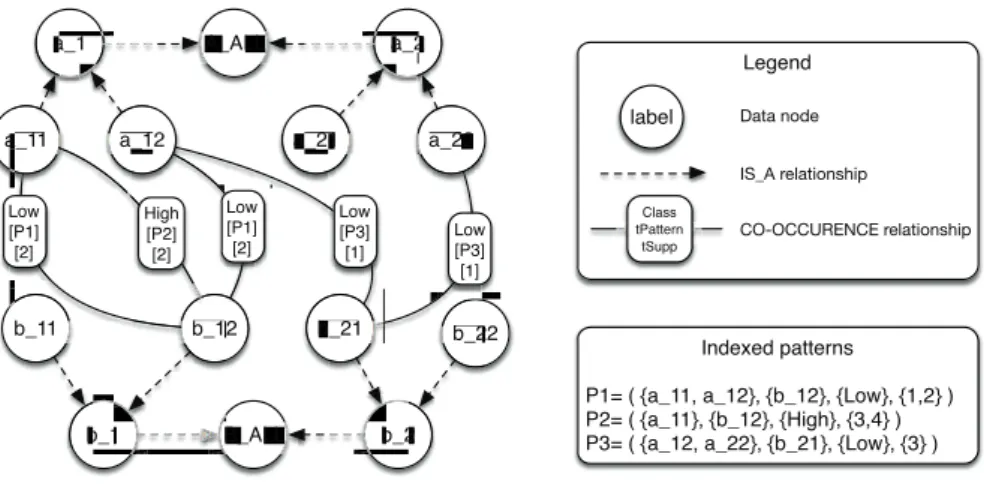
Our method is based on a graph structure for two main reasons. First, hierarchi-cal and membership relationships can be naturally expressed in a graph-based fashion. Second, the rise of NoSQL databases, and especially graph databases, enables a persistent storage of graphs. Such graph databases are particularly of interest in our scenario since we can benefit from indexing techniques, and powerful and efficient SQL-like data manipulation languages. We now detail our model choices.
Vertices are of one single type and represent values of the latent attributes. The set of vertices is denoted V . Given v ∈ V , the function label(v) returns the attribute value represented by v. Two types of relationship co-exist in the graph
structure. First, an arc from v1 to v2 exists if v2 is a direct generalization of v1.
Second, there exists an edge between two data nodes if (1) they do not belong to the same attribute and (2) if there exists at least one pattern where these two nodes co-occur. Some properties are attached to these edges: the class, a list of pattern identifier(s) and a list of pattern support(s). Note that this modeling enables the existence of L edges between two vertices where L is the number of classes. The pattern modeling is less intuitive and will be discussed in Section 5.4. We now formally define these relationship categories.
Definition 5 (The IS A relationship). Let v and v′ be two vertices. There
exists a directed so-called IS A relationship between v and v′, denoted by e =
(v, v′), if Up(label(v), lv(label(v))+1) = label(v’). The set of IS A relationships
is denoted by EI.
Definition 6 (The CO-OCCURING relationship). Let v (resp. v′) be a
vertex with label(v) ∈ Dom(Ai) (resp. label(v′) ∈ Dom(Aj)) and P be a set
of n-ary closed patterns. An undirected so-called CO-OCCURING relationship, denoted by e = (v, v′), exists between v and v′ if a pattern P = (AP
1, . . . , APn, CP,
SuppP) can be found in P such that A
i 6= Aj. Some properties are attached
with such relationships: Class represents one class value associated with P , i.e.,
Class ∈ CP; tP attern is a list of pattern identifiers associated with the class
value Class where v and v′ co-occur; and tSupp is a list that contains the support
of patterns that are stored in tP attern. The set of CO-OCCURING relationships is denoted by EC.
Definition 7 (Graph structure). Let A be a set of attributes and P be a set
of n-ary closed sets. The graph indexing both attribute values and patterns is defined as G = (V, E) with E = EI∪ EC.
Example 5. Figure 3 provides a graphical representation of an example graph
structure considering two dimensions and a given set of n-ary closed sets.
5.3 The Context Matching Operation
The most frequent query that is run to perform classification is to identify
Fig. 3. Graph structure indexing two hierarchical latent attributes and three patterns
the procedure. For ease of reading, it is assumed that we are looking for pat-terns with one specific class i.e., Class = c. The algorithm can, however, be straightforwardly extended to an arbitrary number of classes by repeating this algorithm as many times as the number of class values. Intuitively, the returned set of patterns is the result of the intersection between the edges connecting
every pairs of context attribute values. If there exists ai and aj in a such that
v = (node(ai), node(aj)) is not in VC, it implies that no pattern match the
context a and the algorithm can stop by returning the empty set.
Algorithm 3: Find patterns
Data: a = (a1, . . . , an) a context, c a class value, and G graph structure
patterns← ∅ ; i← 1; F irst← true; while i < n do j ← i + 1 ; while j ≤ n do
if ∃eC = (v, v′)|v = node(ai), v′ = node(aj) and class(eC) = c then
if First then F irst← f alse;
patterns← tP attern(eC) ;
else
patterns← patternsTtP attern(eC) ;
if |patterns| = 0 then return ∅ else return ∅ j ← j + 1; i← i + 1; return patterns
5.4 Discussion
The initial requirements described in Section 5.1 are met for two mains reasons. First, from a technology point of view, graph databases are mature enough to be used as an highly performing replacement solution to relational databases. This choice guarantees persistent storage and an efficient query engine [6]. Second, our model leads to a bounded size and a relatively small number of nodes, i.e., the sum of the latent attribute definition domain size. The number of edges is also relatively small, i.e., a few thousands in our real dataset, compared to the the number of mined n-ary closed sets, i.e., up to some millions. These settings enable Algorithm 3 to perform very efficiently as outlined by our experiment results presented in the next section. Finally, we discuss the non-adoption of another more intuitive graph model. In such an alternative model, patterns would be also represented by vertices and a relationship would exist between a data node and a pattern node if the attribute value represented by the data node belongs to the patterns represented by the pattern node. Despite this alternative model is intuitive, it would significantly increase the time needed to classify a single context. Indeed, in this scenario, the number of vertices in the graph database would be huge. Even if modern servers can deal with such amount of data, this point would be very critical regarding the query phase. Indeed, graph databases are not designed to optimally handle so-called super nodes, i.e., nodes having tens of thousands of relationships. This model has been tried out and most of data nodes were indeed super-nodes, i.e., the density of the graph was closed to 1 (complete graph) leading to very slow (up to some minutes) point-wise query response time. Since the time performance of the approach mainly depends on this query response time, the model has been abandoned.
6
Experimental Evaluation
This section is dedicated to CnSC evaluation. We first detail the adopted protocol and then present and discuss our result.
6.1 Protocol
Dataset. We consider a real dataset from Mobile Broadband Network (MBN). MBN is composed of 600 network nodes (time series producers) which monitor traffic for 5 consecutive weeks at an hourly basis. Traffic load level which repre-sents mobile user activity, allows discretizing nodes into low and high according to traffic level at node. Technical MBN design requires dense node network for
high traffic loads, while during low loads some of the MBN nodes potentially
could be turned off for a temporal period. MBN traffic classification allows es-timating network load at individual network elements and performing network optimization. Three latent attributes and their hierarchical structures are con-sidered: (1) the cell identifier that can be geographically aggregated into sites; (2) the day of the week that is aggregated in either week days or week-end days;
and (3) the hour that is aggregated in periods, i.e., the night, the morning, the afternoon and the evening.
Evaluation Metrics. From an effectiveness point of view, CnSC will be eval-uated using the standard classification measures, the F-measure. From an ef-ficiency point of view, we will study running time and particularly the model building time, i.e., pattern mining and pattern insertion in the graph database, and the average evaluation time per context to classify.
Competitors. CnSC is compared with a previous work, step [13], and the Weka implementation of the Naive Bayes classifier [7].
Evaluated Parameters. We evaluate minSim and minSetSize parameter im-pact on CnSC. minSim is evaluated in the range from 0.1 to 1 with step of
0.1 (0.8 serves as the default value). minSetSize combinations, i.e., vStrong =
(3 5 3 4 1), vN ormal = (2 3 2 3 1), and vSof t = (2 2 2 2 1) (vN ormal serves as
the default value) investigate how the number of mined patters affects results. Implementation and Validation Process. A 10-fold cross validation strat-egy has been used. Results presented in this section are thus averaged. The approach has been implemented in Java 1.7. Data-Peeler software is
imple-mented in C++4. The graph database used in this study is Neo4J (community
release, version 2.0.0)5 as it has been showed in [6] that it offers very good
performances.
6.2 Results
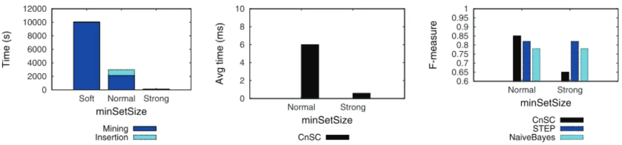
minSetSize Impact. We first evaluate the impact of this parameter on the
model construction time (Fig. 4 (left)). It can be decomposed in two main steps: pattern mining and pattern insertion in the database. The less stringent this constraint, the more important the total time. Most of the time is spent to mine
patterns. Data-Peeler extracts around 40M patterns for vSof t, around 10M
for vN ormal, and only 1K for vStrong. Due to a high number of extracted patterns
with vSof t, the proposed solution failed maintaining the graph structure. For this
reason, setting vSof t is not evaluated in the remaining experiments. The number
of patterns indexed in the graph structure has a big impact on the classification time as stated in Fig. 4 (center). The less patterns, the lower the time to retrieve similar patterns. Moreover, this result shows the great performances of both our algorithms to find similar patterns within the graph and the Neo4j graph databases. Indeed, in the worst case, only 6ms are needed to retrieve patterns with similarity greater than 0.8 within the 10M patterns. From an effectiveness point of view, Fig. 4 (right) shows that the more patterns, the higher the
F-measure. While F-measure is quite low (0.65) with vStrong, it is significantly
better than the two competitors when minSetSize = vN ormal (0.85 against 0.81
for step and 0.78 for the Naive Bayes classifier).
4
It can be downloaded at
http://homepages.dcc.ufmg.br/~lcerf/fr/prototypes.html.
5
0 2000 4000 6000 8000 10000 12000
Soft Normal Strong
Time (s) minSetSize Mining Insertion 0 2 4 6 8 10 Normal Strong Avg time (ms) minSetSize CnSC 0.6 0.65 0.7 0.75 0.8 0.85 0.9 0.95 1 Normal Strong F-measure minSetSize CnSC STEP NaiveBayes
Fig. 4. minSetSizeimpact: decomposition of the running time during the model con-struction (left); average time to classify a single context (center); F-measure (right)
0 10 20 30 40 50 60 70 80 0.1 0.2 0.3 0.4 0.5 0.6 0.7 0.8 0.9 1 Avg time (ms) minSim CnSC 0.6 0.65 0.7 0.75 0.8 0.85 0.9 0.95 1 0.1 0.2 0.3 0.4 0.5 0.6 0.7 0.8 0.9 1 F-measure minSim CnSC STEP NaiveBayes
Fig. 5. minSimimpact: average time to classify a single context(right); F-measure(left)
minSim Impact. The average time required to classify a context is shown in
Fig. 5 (left). Good performances of the average classification time are confirmed. Moreover, as it can be expected, when similarity goes lower, more patterns need to be considered, leading to higher, though acceptable, average classification time. From an effectiveness point of view, two main conclusions can be drawn from Fig. 5 (right). First, when high minSim values are used, too few patterns are considered. This proves the usefulness of taking hierarchies into account to enlarge the context to also include similar ones. Conversely, too low minSim values leads to consider non relevant patterns in the classification process and reduces CnSC accuracy. From Fig. 5 (right) it can be seen that optimal value is
minSim= 0.8. Second, overall performances of CnSC are comparable for most
settings and are significantly better when using the optimal value of minSim.
7
Conclusion
This paper addressed the problems of classifying time series data and presented CnSC, a novel pattern-based approach. Indeed, closed n-ary sets are extracted from latent attributes to serve as maximal context to describe the class value. Hi-erarchical aspect of latent attributes is considered to incorporate similar contexts within the classification process. Use of the graph structure and NoSQL graph database allows a very efficient pattern management and classification time.
With a good parameter setup, i.e., minSim = 0.8 and minSetSize = vN ormal,
Several directions can be taken to extend this work. Among them, we can men-tion automatic estimamen-tion of the best parameter values and concept drift detecmen-tion in the time series distribution to trigger the classification model reconstruction.
References
1. Bringmann, B., Nijssen, S., Zimmermann, A.: Pattern-based classification: A uni-fying perspective. CoRR, abs/1111.6191 (2011)
2. Bringmann, B., Zimmermann, A.: One in a million: picking the right patterns. Knowl. Inf. Syst. 18(1), 61–81 (2009)
3. Cerf, L., Besson, J., Robardet, C., Boulicaut, J.-F.: Closed patterns meet n-ary relations. ACM Trans. Knowl. Discov. Data 3(1), 1–3 (2009)
4. Dong, G., Li, J.: Efficient mining of emerging patterns: Discovering trends and differences. In: Proceedings of the Fifth ACM SIGKDD International Conference on Knowledge Discovery and Data Mining, pp. 43–52 (1999)
5. Gonz´alez, A.B., Ram´ırez Uresti, J.A.: Strategy patterns prediction model (SPPM). In: Batyrshin, I., Sidorov, G. (eds.) MICAI 2011, Part I. LNCS, vol. 7094, pp. 101–112. Springer, Heidelberg (2011)
6. Holzschuher, F., Peinl, R.: Performance of graph query languages: Compari-son of cypher, gremlin and native access in neo4j. In: Proceedings of the Joint EDBT/ICDT 2013 Workshops, pp. 195–204 (2013)
7. John, G.H., Langley, P.: Estimating continuous distributions in bayesian classi-fiers. In: Eleventh Conference on Uncertainty in Artificial Intelligence, pp. 338–345 (1995)
8. Li, W., Han, J., Pei, J.: Cmar: accurate and efficient classification based on multiple class-association rules. In: Proceedings of the 2001 IEEE International Conference on Data Mining, pp. 369–376 (2001)
9. Liu, B., Hsu, W., Ma, Y.: Integrating classification and association rule mining. In: Proceedings of the Fourth International Conference on Knowledge Discovery and Data Mining, pp. 80–86 (1998)
10. Monreale, A., Pinelli, F., Trasarti, R., Giannotti, F.: Wherenext: A location pre-dictor on trajectory pattern mining. In: Proceedings of the 15th ACM SIGKDD International Conference on Knowledge Discovery and Data Mining, pp. 637–646 (2009)
11. Quinlan, J.R.: C4. 5: programs for machine learning, vol. 1. Morgan Kaufmann (1993)
12. Rao, D., Yarowsky, D., Shreevats, A., Gupta, M.: Classifying latent user attributes in twitter. In: Proceedings of the 2nd International Workshop on Search and Mining User-generated Contents, pp. 37–44 (2010)
13. Samulevicius, S., Pitarch, Y., Pedersen, T.B., Sørensen, T.B.: Spatio-temporal en-semble prediction on mobile broadband network data. In: 2013 IEEE 77th Vehicular Technology Conference, pp. 1–5 (2013)
14. Wang, J., Karypis, G.: Harmony: Efficiently mining the best rules for classifica-tion. In: Proceedings of the Fifth SIAM International Conference on Data Mining, pp. 205–216
15. Yavas, G., Katsaros, D., Ulusoy, ¨O., Manolopoulos, Y.: A data mining approach for location prediction in mobile environments. Data Knowl. Eng. 54(2), 121–146 (2005)