Experimental and numerical study of two-phase flows in arrays of cylinders

O

pen

A

rchive

T

OULOUSE

A

rchive

O

uverte (

OATAO

)

OATAO is an open access repository that collects the work of Toulouse researchers and

makes it freely available over the web where possible.

This is an author-deposited version published in :

http://oatao.univ-toulouse.fr/

Eprints ID : 9392

To link to this article : DOI:10.1016/j.ces.2013.08.031

URL :

http://dx.doi.org/10.1016/j.ces.2013.08.031

To cite this version : Horgue, Pierre and Augier, Frédéric and Duru,

Paul and Prat, Marc and Quintard, Michel. Experimental and numerical

study of two-phase flows in arrays of cylinders. (2013). Chemical

Engineering Science, vol. 102. pp. 335-345. ISSN 0009-2509

Any correspondance concerning this service should be sent to the repository

administrator:

staff-oatao@listes-diff.inp-toulouse.fr

Experimental and numerical study of two-phase flows in arrays

of cylinders

Pierre Horgue

a,c,n

, Frédéric Augier

c

, Paul Duru

a

, Marc Prat

a,b

, Michel Quintard

a,b

a_{Université de Toulouse, INPT, UPS, IMFT (Institut de Mécaniques des Fluides de Toulouse), Allée Camille Soula, F-31400 Toulouse, France} b_{CNRS, IMFT, F-31400 Toulouse, France}

c_{IFP Energies Nouvelles, rond-point de l'échangeur de Solaize, BP 3, 69360 Solaize, France}

a b s t r a c t

In this paper we study the spreading of a liquid jet in a periodic array of cylinders with a characteristic size of the passages between solid obstacles equal to 1.5 mm, close to the capillary length. An important outcome of our study is to show that this configuration allows most of the two-phase flow regimes described in the literature about trickle beds to be observed, even with no gas injection. Different aspects of the flow phenomenology have been studied, such as bubble creation and transport. As direct numerical methods for tracking interfaces would require too much computation time, especially in three-dimensional cases, we propose to simulate the two-phase flows observed experimentally with two-dimensional simulations corresponding to the spreading of a liquid jet in an array of disks. We show that this numerical approach allows the phenomenology observed experimentally to be reproduced satisfactorily. Hence, numerical simulations can be used subsequently to study the effects of specific parameters without setting up a new experimental procedure. As an example, the stabilizing effect of gas injection on the flow pattern is studied numerically.

1. Introduction

Gas–liquid downward flows are common in chemical reactors (Lee and Pang Tsui, 1999). When a stationary solid phase is involved, different hydrodynamic regimes can occur depending on the flow rate and properties of each phase. This is the case in fixed bed catalytic reactors (Larachi et al., 1991) commonly used in the refining industry for the hydroprocessing of petroleum cuts. In such reactors, spherical or extrudate catalyst particles of 1–4 mm of diameters are generally used. Following previous studies (Charpentier and Favier, 1975; Ng and Chu, 1987), 4 different

regimes are identified, but the most common regime is the trickling one. Despite simple flow characteristics in Trickle Bed Reactors (TBRs), hydrodynamic behavior of such reactors has been the object of many studies (Al-Dahhan et al., 1997). This is partly due to the high sensitivity of local flow patterns to physical properties of the fluids and solid phases, in addition to interface properties as contact angles and surface tensions (Baussaron et al., 2007; Julcour-Lebigue et al., 2009). In particular, exact position of transitions between well characterized regimes as trickling, bubbly or pulsed regimes are not exactly known. Moreover, physical mechanisms responsible of regime modifications and transitions are not completely understood and modeled. Maldistributions in TBRs are known to be very difficult to avoid completely while being responsible of important losses of reaction efficiency (Strasser, 2010). They can be generated by poor homogeneity in either the loading of catalyst particles, the distributors at the top of

n

Corresponding author at: Université de Toulouse, INPT, UPS, IMFT (Institut de Mécaniques des Fluides de Toulouse), Allée Camille Soula, F-31400 Toulouse, France. Tel.: þ33 534 322 855.

reactors, or both. In either case, complex flow redistribution mechanisms are involved. Non-invasive experimental techniques have been successfully applied to investigate TBRs, such as

γ

"tomography (Reinecke and Mewes, 1997; Schubert et al.,

2008), ECT (Matusiak et al., 2010) or collecting devices at the bottom of columns (Marcandelli et al., 2000), but they are generally limited to analysis scales larger than catalyst particle length.

Pursuing the main objective of modeling flows inside TBRs, a first step consists in the study of the trickling flow in a quasi 2-dimensional configuration of an array of cylinders. The flow generated inside this configuration is appropriate to observe transition mechanisms that are also present inside complex 3-dimensional flows, like bridges between trickling liquid films. As the 2D setup is easy to investigate using optical techniques, this presents a good case to validate numerical modeling approaches that may be further used to simulate downward gas/liquid flows in 3-dimensional fixed bed of solid particles. The chosen configura-tion is reminiscent of the case of tube bundles and it is therefore interesting to examine the literature on this subject.

Two-phase flows in tube bundles, from microchemical reactors to heat exchangers, have been extensively studied because of the many industrial processes that are based on this geometry. Each process features specificities depending on the operating condi-tions such as the pressure, the temperature or the characteristic size of the system. In microfluidic devices, with a much smaller gap between solid obstacles than the capillary length, the capillary forces are dominant when compared to the gravity force. On the contrary, if we consider a heat exchanger composed of a tube bundle with a characteristic gap of about 1 cm, the capillary forces may be neglected compared to the gravitational force and often compared to inertial effects as well. The flow regimes, their properties, and the transitions between them, have been the purpose of many studies (Kondo and Nakajima, 1980; Ulbrich and Mewes, 1994; Xu et al., 1998; Noghrehkar et al., 1999) but remain poorly understood in the case of tube bundles. The major objective of any modeling attempt is to determine pressure drops and phase fractions which are intimately associated with the observed flow pattern.

The characterization of the flow patterns and their transitions has been studied experimentally by previous authors for different flow conditions, upward or downward, and for different tube arrangements, in-line or staggered. Flow regime maps have been plotted first for upward flow in staggered tube bundles (Kondo and Nakajima, 1980), then for an in-line arrangement (Ulbrich and Mewes, 1994). Xu et al. (1998) studied up and down-flow in an in-line tube bundle and Noghrehkar et al. (1999) studied the effect of the arrangement by performing experiments on both in-line and staggered tube bundles. Melli et al. (1990) draw flow regime maps in “two-dimensional” packed beds composed of a staggered arrangement of O-ring solids placed between two plates. The objective of that study was to simultaneously observe regime transition at the microscale, i.e. the scale of the passage between two solids, and in the O-ring bundle at the macro-scale,. More recently, Krishnamurthy and Peles (2007) studied the flow pat-terns for two-phase flows through a staggered bank of micro-pillars and highlighted the differences with previous studies at a larger scale. We must note that the flow maps, plotted in different experimental conditions and at different scales, have the same trends. However, phenomena related to flow regime changes at the scale of a tube bundle remain too poorly understood to develop general regime change laws.

Due to the various flow patterns that can exist in tube bundles, the influences of which are not fully assessed, modeling approaches to predict pressure drop and void fraction are generally empirical. Most of them are based on an adaptation of

existing models, for instance in-tube two-phase flow models. The most commonly used approach is based on the Lockhart–Marti-nelli model (Lockhart and MartiLockhart–Marti-nelli, 1949) which relates the two-phase pressure drop to the one-two-phase pressure drop, through specific correlations. This approach was first developed for two-phase flow in pipes and then used for more complex geometries, including tube bundles. Such models have been used successfully for vertical up and down flows across horizontal tube bundles (Xu et al., 1998) and for gas–liquid flows across a bank of micropillars (Krishnamurthy and Peles, 2007). The effect of the pitch-to-diameter ratio (the pitch is the distance between the centers of two neighboring tubes in the tube bundle) was also studied for staggered and in-line tube bundles (Dowlati et al., 1992). Recently, Bamardouf and McNeil (2009) performed a comparison between various correlations available in the literature and found that the most accurate prediction in terms of void fraction is given by Feenstra et al. (2000) correlation and that Ishihara et al. (1980) correlation is the best way to predict the pressure drop.

Some numerical studies concerning the flow modeling at the pore scale, i.e. the scale of the passage between tubes, have been performed in an effort to understand more accurately the origin and transitions of the different regimes. The two-phase flow modeling at low Reynolds numbers, in which interfaces play an important role and need to be explicitly tracked, is a complex case due to numerical issues. Direct numerical methods for tracking interfaces, such as the “Volume-of-Fluid” method (Hirt and Nichols, 1981), have been successfully used to simulate two-phase flow in tubes (Gupta et al., 2009). However, even with a significant reduction of the computation time due to the axial symmetry of the problem, simulations still requires significant computation time. More recently, the Volume-Of-Fluid method has been validated in a three-dimensional case, the trickling flow on a stack of a few particles (Augier et al., 2010). However, this was possible for a small number of “grains” only and required long computation times (around one week on 2 processors for 1 s of physical time). The numerical simulation of two-phase flows at the scale of a tube bundle requires too much computation time under these conditions, which explains the lack of numerical simulations.

The experimental configuration used in this work is first presented in Section 2.1. It is based on the use of micromodels consisting in arrays of cylinders maintained within a Hele Shaw cell. The characteristic lengths of the system (cell thickness and minimum spacing between neighboring cylinders) are 1.5 mm, close to the capillary length for most fluids, which allows for an interesting competition between capillary, gravity, and inertial effects. Considering that the experimental device can be seen as a two-dimensional medium, two-dimensional numerical simula-tions on array of disks were performed using a numerical interface tracking method, namely the “Volume-Of-Fluid” method,

imple-mented in the OpenFOAMs_{software, as described in Section 2.2.}

As already mentioned, direct numerical simulations are very time consuming, particularly in three-dimensions, which prevent the possibility to simulate the two-phase flow in the real geometry of the experiment with reasonable computation times. The constitu-tive equations of the present 2D numerical model have therefore been modified by adding terms which account for the three-dimensional effects present in the experimental device using simplifying assumptions. The visualization of spreading of a liquid jet injected in the micromodels led to the observation of different flow regimes, similar to those usually observed in trickle beds or in tube bundle flows, which were dependent on the injection flow rate. Both regime transitions and flow patterns properties are described in Section 3. The numerical results presented in Section 4 compare favorably with the experimental results, which confirm the ability to simulate the experimental phenomenology with a

purely two-dimensional approach. The 2D numerical model is then used to study the effect of gas injection on the spreading of the liquid jet, a study that would have been more involved to set up experimentally. Conclusions are drawn in Section 5.

2. Experimental and numerical methods

In this section, we describe the experimental setup and the associated mathematical problem we solved using numerical

procedures implemented in OpenFOAMs

. 2.1. Experimental setup

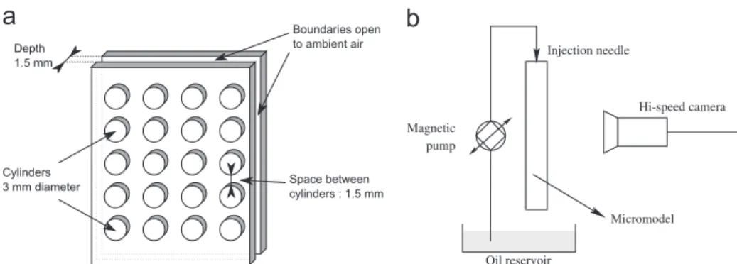
The experimental setup is schematically represented in Fig. 1. The micromodels used consist of in-line arrays of cylinders, each cylinder having a diameter of 3 mm and a height of 1.5 mm. Each micromodel was made of polydimethylsiloxane (PDMS, Silicon Elastomer, Sylgard): the textured layer was first obtained by pouring liquid PDMS in a machined plexiglas negative mould, baking it in an oven (1 h, 65 1C) and then removing it from the mould. It was then placed on top of another flat layer of PDMS that was previously partially cured (20–30 min at 65 1C). The two assembled layers were then cured for another 30 min at 65 1C to obtain a definitive bonding. Note that the lateral boundaries of the transparent micromodel thus obtained are open to ambient air.

The fluid used is a silicon oil (Silicon M5, Roth), with mass

density

ρ

¼ 0:92 $ 103kg m"3 _{and dynamic viscosity}

_μ

_{¼ 5$}

10"3_{Pa s. The oil–air surface tension is s ¼ 0:032 N m}"1_{. The oil}

is perfectly wetting on the PDMS surface. The experimental device is held vertically and oil is injected on top of a cylinder using a flat needle. Liquid flow rates through the needle are controlled using a laboratory gear pump (BVP-Z, Ismatec) in a range from 1 to

40 cm3_min"1_{(see Fig. 1b).}

The Bond number is defined as Bo ¼

ρ

gL2=s where the length L

is taken as the micromodel thickness (L ¼ 1:5 mm). For the present

experiment, Bo ¼ 0:63. The capillary number is defined as

μ

VSL=s

where VSLis the interfacial fluid velocity, defined as the flow rate

divided by 2 $ 1:5 $ 1:5 mm2 _{(see Section 3). Capillary numbers}

are in the range 5:8 $ 10"4_{to0:022. Reynolds numbers, Re ¼}

ρ

VSL

L=

μ

, are in the range 1–40.

Visualizations are done using a high-speed camera (Dimax,

PCO) with a 2048 $ 2048 pixels2 CMOS sensor, the system being

backlighted with a white LED panel (Phlox). The frame acquisition rate was typically set to 200 frames per seconds with an exposure time set to 1/200 s.

2.2. Numerical approach

Interface tracking methods have been extensively developed recently in parallel with the improvement of computational

capabilities. Two main approaches may be considered to predict interface displacements for two-phase flows. The Lagrangian methods, which discretize explicitly the interface and track the node displacements, and the Eulerian methods, which transport a volume fraction scalar representing the proportion of each fluid in a cell of a fixed mesh. The method chosen for this study is an Eulerian diffuse-interface method, the Volume-Of-Fluid (VOF) method, which is more suitable that Lagrangian methods to simulate dramatic changes in the interface configuration, espe-cially coalescence and snap-off. This ability to handle interface appearance or disappearance will be particularly useful to simu-late the coalescence of liquid films occurring during the spreading of the liquid jet. We first present the VOF model as implemented

in the OpenFOAMs

software. Then, we introduce a modified VOF formulation, including additional terms which take into account the three-dimensional effects of the experimental device in two-dimensional numerical simulations. In the VOF method, the flow of two immiscible fluids is governed by a single set of Navier– Stokes ∂ ∂tð

ρ

vÞ þ ∇ ' ð

ρ

vvÞ ¼ "∇p þ∇ ' ½

μ

ð∇v þ ∇v T_{Þ) þ}

_ρ

_{g þ F} vol; ð1Þ ∇_{' v ¼ 0: ð2Þ}

The Fvol term in Eq. (1) represents the effect of the interfacial

tension taken into account using a continuum formulation (Brackbill et al., 1992)

Fvol¼ s

κ

∇

α

; ð3Þ

where s is the interfacial tension between the two fluids and

κ

the

curvature at the interface, defined in terms of the divergence of

the unit normal to the interface ni

κ

¼ ∇ ' ni: ð4Þ

The fluid properties are calculated within each cell using the

volume fraction,

α

ρ

¼

αρ

_liquidþ ð1"

α

Þ

ρ

_gas; ð5Þ

μ

¼

αμ

_liquidþ ð1"

α

Þ

μ

_gas: ð6Þ

The volume fraction

α

is transported using the VOF equation

∂

_α

∂tþ ∇ ' ð

α

uÞ þ ∇ ' ð

α

ð1"

α

ÞurÞ ¼ 0; ð7Þ

where is u the fluid velocity. ∇ ' ð

α

ð1"

α

ÞurÞ is an artificial

com-pression term used to prevent the numerical diffusion which tends to smear the interface sharpness (see Rusche, 2002). In this model,

the formulation of the compression velocity ur is based on the

maximum velocity magnitude in the transition region.

In order to capture accurately, with interface-diffuse methods, some two-phase phenomena such as liquid films along the cylinders, it is necessary to refine the mesh significantly. Fig. 1. Experimental setup. (a) Micromodel, (b) Schematic representation of the setup.

A previous study (Horgue et al., 2012) has shown that accurate simulations of liquid film flow required at least two grid cells in the film. As we are interested in the simulation of different flow regimes, interfaces can be located anywhere in the domain and, therefore, it is quite impossible to decide where to refine locally the mesh. As a consequence, we used an unstructured mesh with a

characteristic cell size about 50

μ

m for the simulations presented

in this paper. The 2D grid mesh representing the experimental

device is composed by about 105_{cells and one second of}

physical-time simulation requires between 20 and 40 h of computation time (with 8 processors at 2.4 GHz). Simulating the experiment in three dimensions with an equivalent characteristic cell size would induce computation times at least 30 times greater.

For this reason, it is interesting to simulate the two-phase flow in the micromodel with a purely two-dimensional numerical model taking into account three-dimensional effects occurring in the experimental device. It has been demonstrated for Hele-Shaw cells that a 2D model involving cross-section averaged quantities may be used to that end (Park and Homsy, 1984). Here, the impact of the no-slip condition along the micromodel front and back plates and the impact of the interface curvature in the plane perpendicular to the flow are considered. The no-slip condition effects are taken into account by modifying the momentum equation of the 2D VOF model (1) as follows:

∂ ∂tð

ρ

vÞ þ∇ ' ð

ρ

vvÞ þ

μ

Kv ¼ "∇p þ ∇ ' ½

μ

ð∇v þ ∇v T_{Þ) þ}

ρ

g þFvol; ð8Þ

where

μ

=Kv is an additional term, inherited from a porous medium formulation, and classically used in Hele Shaw modeling. This approximation is acceptable for a sufficiently low Reynolds number and a position within the Hele-Shaw cell far enough from the meniscus or obstacles. In this case, the velocity profile between the plates follows a Poiseuille law and we can express the equivalent permeability K as:

K ¼h 2

12; ð9Þ

where h is the Hele-Shaw gap between the two plates.

The modifications of the 2D model due to the impact of the meniscus curvature were studied by Park and Homsy (1984), using matched asymptotic developments. In the experimental device,

the local interface curvature is the sum of two main curvatures:

κ

xy

in the 2D simulation plane and

κ

zin the plane perpendicular to the

flow. Considering that the interface is at equilibrium for the

κ

z"plane and that the PDMS is perfectly wetted by the oil phase,

the curvature in this plane can be formulated as a function of the Hele-Shaw gap h. With these assumptions, the interface curvature

in the 2D model can be expressed as follows:

κ

¼

κ

xyþ

κ

z¼ ∇ ' niþ

2

h ð10Þ

It is important to understand at this point that the modified 2D model is only an approximation of the 3D real situation, and that some complex 3D flows near the meniscus, or in the neighborhood of the obstacles, are not exactly reproduced. We will come back to this point later.

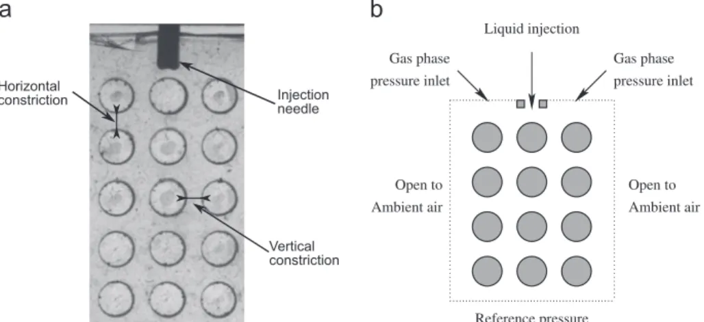
The simulation conditions are summarized in Fig. 2b, with at the bottom, an atmospheric reference pressure, and, at the top, a velocity inlet condition for the central oil injection. Top and lateral boundaries for the gas phase are open to ambient air.

3. Experimental results: characterization of flow regimes Several experiments were performed at various flow rates: four different flow regimes were observed depending on the liquid flow rate. The observed two-phase flow patterns correspond qualitatively to those usually described in the literature on trickle beds. Three of these regimes are steady-state regimes: the trickling, bridged and flooded regimes; while one is unsteady (the pulsing regime).

In order to illustrate these findings, we focus in the following on the spreading of the liquid jet on three columns of the array of cylinders considered in the present study. The liquid is injected on top of the central, up cylinder and flows downward in the right and left “channels” delimited by the central column of cylinders and the two lateral ones. Consequently, the liquid superficial

velocity VSLused to quantify the transitions between the different

flow regimes is defined as the injection flow rate divided by twice the section of a channel (at the level of a constriction), that is

2 $ 1:5 $ 1:5 mm2_.

In the following, a distinction is made between the experi-ments performed with a “dry” micromodel, i.e., a micromodel not previously used and those performed with a “pre-wetted” micro-model, i.e., the internal surface of which has been already exposed to the perfectly wetting silicon oil. In this case, the experimental device which has been flooded by oil once is let to drain under gravity for several minutes before a new experiment is started. The experimental device is not manipulated between “dry” and “pre-wetted” experiments, and the observed differences are exclusively related to the presence or the absence of liquid films in the micromodel.

3.1. Flow regimes in a dry micromodel

With a dry micromodel, for the lowest liquid flow rates, the flow regime is characterized by the trickling of the liquid as a film

along the central column of cylinders (see Fig. 3a, VSL¼

0:011 m s"1_{). The trickling liquid film thickens symmetrically when}

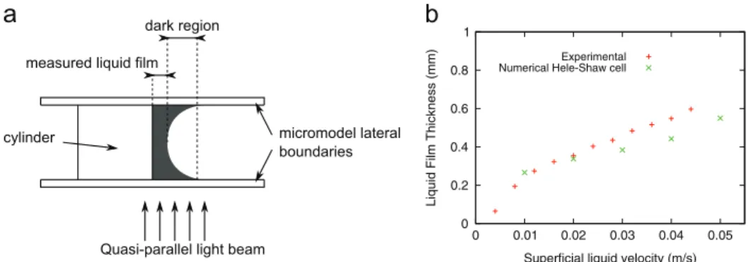
the flow rate is increased (before any transition to another flow regime, see below) and the film thickness can be measured as the distance between a given cylinder edge (at a constriction) and the side of the dark region on the image that is the closest to the considered cylinder, the dark region being optically caused by the deviation of the quasi-parallel light beam from the led panel by the meniscus between the liquid film and the micromodel walls, see the side view sketch in Fig. 4a. Fig. 4b shows the liquid film thickness as a function of the liquid superficial velocity.

When the flow rate is increased, some static liquid bridges can appear between two cylinders belonging to neighboring columns and the channel between the two columns is hence in a bridged regime

(Fig. 3, right channel for VSLbetween 0:051 m s"1and 0:106 m s"1).

During the liquid bridge formation, a local instability can make the liquid films in an horizontal constriction between two cylinders coalesce, thus trapping a gas bubble which eventually moves down through the channel. The liquid films in the con-striction where the first bubble was generated remain unsteady, generating a regular bubble train flowing down. The flow regime

in this column is then called a pulsing regime. The same kind of liquid bridge destabilization can also be observed from an estab-lished liquid bridge, for a sufficiently high flow rate. For instance, the left column of cylinders in Fig. 3a reaches directly the pulsing

regime at VSL40:051 m s"1 while the right column is in the

bridged regime for VSL in the range 0:051–0:106 m s"1 before

transiting to a pulsing regime as soon as VSL40:106 m s"1(see

Fig. 3b). In the pulsing regime, the bubble formation is periodic: successive images illustrating a single liquid bridge pinch-off leading to a bubble formation are shown in Fig. 5a. It is found that, once the pulsing regime is established in a given channel between two columns, the bubbles size decreases when increasing the liquid flow rate above the threshold for the transition observed for this particular channel. A “large” bubble must deform signifi-cantly in order to pass the constriction (see Fig. 6a, left). This

interface deformation involves different behaviors of the

bubble velocity profiles of the front and the rear of the bubble, as depicted in Fig. 6. The bubble front and rear velocities were measured from images recorded at 200 fps (note that velocity variations observed at the front of the bubble are then much smaller than those of the back). When the bubble diameter is smaller than the constriction diameter (at higher flow rates), the bubbles accelerate when they move through a constriction between two cylinders, while deforming very slightly, as can be seen in Fig. 6b.

Fig. 3. (a) Flow regimes visualizations in a dry micromodel, as a function of the superficial velocity VSL. (b) Flow regime map for the left and right channels. The flow in the micromodel is unsteady (grey area on the figure) when at least one column is in the pulsing regime.

Once the pulsing regime is reached in a column, increasing the liquid flow rate reduces the bubble sizes and finally leads to a flooded regime, as illustrated in Fig. 3a (flooded regime between

the left and central columns of cylinders as soon as

VSL40:071 m s"1 and between the right and central columns of

cylinders for VSL40:150 m s"1). It is worth noticing that we did

not observe in the present experiments a transition from the pulsing regime to the bridged regime when the flow rate is decreased (from a situation where the pulsing effect is estab-lished). Actually, the interface instability generating the gas bubbles persists even when decreasing the liquid injection flow rate below the threshold found for the transition from the bridged to the pulsing regime in the channel considered. The flow regime transition then observed while decreasing the flow rate is always from the pulsing to the trickling regime. This hysteresis effect on the regime transitions is probably due to the presence of a persistent liquid film along the wall and at the corners that substantially alters the wettability effect.

In Fig. 3b, the flow regime thresholds observed for the experi-ments for which the focus was on three columns of cylinders only are summed up as a function of the liquid superficial velocity. These transition thresholds were found to vary by less than 5%

when performing four times the experiments using four different dry micromodels.

3.2. Flow regimes in a pre-wetted micromodel

In the case of a pre-wetted micromodel, capillarity-trapped, static, thin liquid films around the cylinders can be observed prior to liquid injection. This has a huge impact on the transitions between the flow regime, which is a well-recognized fact in the trickle bed literature (Ng and Chu, 1987; Saroha and Nigam, 1996; Ranade et al., 2011). As for the experiment in the previous case (dry micromodel), the observed configurations for various velocities are represented in Fig. 7a, and the regime transitions, depending on the liquid superficial velocities, are presented in Fig. 7b. For the lowest liquid superficial velocities

(VSLo0:01 m s"1), we observe the trickling regime around the central

column of disks. Then, when increasing the liquid injection, the static liquid films around the cylinders, remaining after the drainage process, cause the creation of liquid bridges at very low liquid superficial

velocities compared to the dry case (around VSL¼ 0:01 m s"1 to be

compared to VSL¼ 0:051 m s"1 for a dry micromodel). For a low

injection rate, VSL¼ 0:014 m s"1, the system becomes unsteady for

the observed two channels (pulsing flow regime). This corresponds to Fig. 4. (a) Definition of the trickling film thickness: side view sketch. (b) Liquid film thickness in the trickling regime as a function of VSL.

Fig. 5. Pinch-off mechanism leading to the formation of a bubble for various times: (a) Experimental visualizations, (b) Numerical simulations (liquid phase in red and gas phase in blue). (For interpretation of the references to color in this figure caption, the reader is referred to the web version of this paper.)

a much lower transition than for the dry experiments. Similarly to what is observed in the dry case, increasing the liquid superficial velocities tends to reduce the sizes of the bubbles, before reaching a steady, flooded regime for the same velocity as in the dry case

(VSL¼ 0:150 m s"1).

4. Direct numerical simulations (DNS) results

The objective of this section is to evaluate the ability of the 2D numerical model to reproduce the phenomenology observed experimentally. First, results comparing the DNS to the experi-mental observations are presented. Then, DNS is used to model a situation not studied experimentally, when gas is injected along-side with the liquid.

4.1. Comparison with experiments

By increasing progressively the liquid flow rate, we qualita-tively obtain flow regimes which are similar to those observed experimentally, as illustrated in Fig. 8 and detailed below.

For the lowest liquid injection rate, a trickling film regime is obtained. The shapes of the interfaces obtained with the 2D simula-tions are similar to those observed in the dry experimental device

(compare Fig. 3a, for VSL¼ 0:011 m s"1, and Fig. 8a). Moreover, the

liquid film thickness obtained numerically is in good agreement with

the experimental measurements for VSLo0:025 m s"1, see Fig. 4b. For

larger superficial velocities, the agreement deteriorates as VSLincreases

but the discrepancy remains less than 25%.

The formation of the first liquid bridges arises for a superficial

liquid velocity close to 0:10 m s"1_{(to be compared with the dry}

experimental threshold, VSL¼ 0:05 m s"1). It can be noticed that

the liquid bridges in the 2D simulations are not static but “fall down” to the bottom of the simulated numerical domain.

As observed in the experimental case, a further increase in the liquid flow rate causes a transition to a periodic pulsing regime in each channel, with traveling bubbles sizes decreasing when increasing the flow rate beyond transition (see Fig. 8, at

VSL¼ 0:15 m s"1 and at VSL¼ 0:20 m s"1). Note that the pulsing

regime occurs directly in the two channels in DNS, as observed experimentally in the pre-wetted micromodel. As shown in Fig. 5b, the present two-dimensional simulations correctly capture the bubble creation process which occurs at the top of the cylinder array. Similarly, bubble deformation and front and rear interface periodic velocity variations, are similar to those observed in the experiment for small and large bubbles, see Fig. 6.

At VSL¼ 0:22 m s"1 (Fig. 8), one column is flooded while the

other column stays in a pulsing regime. A similar situation was previously observed in the experiments for a liquid superficial

velocity VSL* 0:11 m s"1. Finally, the totally flooded regime

occurs at VSL¼ 0:25 m s"1in numerical simulations and at VSL¼

0:15 m s"1_{for the experimental cases.}

To recap this comparison between the present DNS results and the experimental ones, we can first say that the flow patterns observed are similar in both cases (with the notable exception that falling liquid bridges are obtained only numerically). The main differences observed concern the precise values for the thresholds for transitions from one flow regime to another. The trickling regime is notably observed for a

much larger VSL range. The transition to a pulsing regime occurs

Fig. 6. Bubble flow through the micromodel. (a) Case of a large bubble. Left: experimental and numerical visualizations, Center and Right: experimental ðVSL¼ 0:111 m s"1Þ and numerical (VSL¼ 0:180 m s"1) bubble front and rear interfaces velocities observed when the bubble is flowing down in between two columns of cylinders. (b) Case of a small bubble. Left: experimental and numerical visualizations, Center and Right: experimental ðVSL¼ 0:126 m s"1Þ and numerical (VSL¼ 0:220 m s"1) bubble front and rear interfaces velocities observed when the bubble is flowing down in between two columns of cylinders. The bubble velocity is made dimensionless by dividing by the average bubble velocity.

simultaneously in the two channels for the DNS case, which may be a reflection of the perfectly regular simulated flow geometry by opposition to the experimental case.

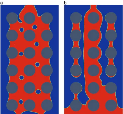
We believe that the differences between DNS and experi-ments are due to the fact that the proposed 3D corrections to the present 2D VOF approach may not incorporate all 3D effects. This is emphasized by the fact that, even if the 3D corrections do not catch all 3D effects, they do have an impact. Indeed, Fig. 9 shows the influence of the 3D effects in the simulations by comparing numerical simulations with the purely 2D VOF model and the modified formulation taking into account (approximately) 3D

effects (see Section 2.2), for VSL¼ 0:20 m s"1. The latter case is in

much better agreement with the experimental observations showing the critical nature of the 3D corrections proposed. The correction proposed in Eq. (10) only takes into account additional

curvature effects when

κ

xyis small compared to h"1. Additional

3D effects not taken into account by this correction are listed below:

+

_{dynamic films already presents or developing during the flow,}

+

vortices near the meniscus,

+

complex menisci arising near the obstacles,…

A formal quantitative analysis of these effects is beyond the scope of this paper and would require to develop higher order correc-tions for the 2D VOF model (a difficult task for flows around

menisci or obstacles), or perform 3D simulations (which is difficult because of the required mesh size, as explained earlier in this paper).

To conclude, the global agreement between the experiments and the 2D simulations remains nonetheless satisfactorily, so that the numerical approach may be used with some confidence to study and understand more precisely the physical phenomena involved in the present situation. To illustrate this point, we present below some results concerning the impact of gas injection on the pulsing flow regime.

4.2. Influence of gas injection

To illustrate the possibilities offered by the numerical approach, we performed direct numerical simulations with a small pressure drop imposed for the gas phase to qualitatively observe the influence of the resulting gas flow on the liquid jet, for a single

fluid interfacial velocity VSL¼ 0:15 m s"1 (pulsing regime, see

Fig. 8). For these simulations, lateral boundary conditions were set to solid walls, placed on both sides of the right and left cylinders column, 1.5 mm away from the cylinders external edge. As far as the spreading of the liquid jet is concerned, no effects are found as far as the gas pressure drop is smaller than 30 Pa

(which correspond to gas superficial velocities less than 1 m s"1_).

For higher pressure drops, gas injection hinders the bubble creation process in the left channel: an elongated gas slug Fig. 7. (a) Flow regimes visualizations in a pre-wetted micromodel as a function of the superficial velocity VSL. (b) Flow regime map for the left and right channels. The flow in the micromodel is unsteady (grey area on the figure) when at least one column is in the pulsing regime.

progressively forms in the channel and extends until a trickling regime is established on the left side of the cylinders of the central column while some static liquid bridge remains in between the cylinders of the left column (see Fig. 10). Similarly, it is found that, starting with a flooded regime, gas injection provokes, at suffi-ciently high pressure drops, the disconnection of the two external cylinders column from the central one, around which a trickling film subsists (data not shown).

5. Conclusion

The spreading of a liquid jet across in-line arrays of cylinders was experimentally and numerically studied in the case of a micro-model. The characteristic length of the passages between cylinders was chosen to be close to the capillary length. The combination of gravity and capillary effects in this case allowed most of the flow regimes described in the trickle bed literature to be observed, even with no gas injection. Once this representative-ness of the “2D trickle bed” is established, this is interesting to take advantage of the possibility of closer and better observations to understand more deeply the different mechanisms occurring in

such situations. For instance, the hysteresis effect of pre-wetting the experimental device on the flow regime transitions has been observed in details.

We also have shown that it is possible to simulate the flow phenomenology observed during the experiment with two-dimensional simulations, with some differences in time and space scales due to the difficulty in incorporating all 3D effects in the 2D model. Bearing in mind these quantitative differences, this is nonetheless particularly interesting to look at these results, since a numerical approach presents many advantages. It can be used to observe the influence of one particular parameter without having to set up a new experimental procedure. For each simulation, we have at our disposal, for interpretation purposes, the internal fields (pressure, velocity, interface positions), which are difficult to measure experimentally. We observed, for example, the stabilizing effect of air injection in the cylinder bundle with the help of these numerical simulations. In conclusion, since direct numerical simu-lations of the real problem in three dimensions would require too much computation time, we suggest to use instead the 2D averaged model, since we have established that these 2D simula-tions reproduce most of the features required to better understand trickle bed physics. Moreover, such a numerical approach may be Fig. 8. Flow regimes observed with the Volume-Of-Fluid method.

used as a development basis to simulate more complex multiphase flows, including, for example, multicomponent mass transfer, heat transfer or phase change.

References

Al-Dahhan, M.H., Larachi, F., Dudukovic, M.P., Laurent, A., 1997. High-pressure trickle-bed reactors a review. Industrial & Engineering Chemistry Research 36 (8), 3292–3314.

Augier, F., Koudil, A., Royon-Lebeaud, A., Muszynski, L., Yanouri, Q., 2010. Numerical approach to predict wetting and catalyst efficiencies inside trickle bed reactors. Chemical Engineering Science 65, 255–260.

Bamardouf, K., McNeil, D.A., 2009. Experimental and numerical investigation of two-phase pressure drop in vertical cross-flow over a horizontal tube bundle. Applied Thermal Engineering 29 (7), 1356–1365.

Baussaron, L., Julcour-Lebigue, C., Wilhelm, A.-M., Delmas, H., Boyer, C., 2007. Wetting topology in trickle bed reactors. AIChE Journal 53 (7), 1850–1860. Brackbill, J.U., Kothe, D.B., Zemach, C., 1992. A continuum method for modeling

surface tension. Journal of Computational Physics 100, 335–354.

Charpentier, J.-C., Favier, M., 1975. Some liquid holdup experimental data in trickle-bed reactors for foaming and nonfoaming hydrocarbons. AIChE Journal 21 (6), 1213–1218.

Dowlati, R., Chan, A.M.C., Kawaji, M., 1992. Hydrodynamics of two-phase flow across horizontal in-line and staggered rod bundles. Journal of Fluids Engineer-ing, Transactions of the ASME 114 (3), 450–456.

Feenstra, P., Weaver, D., Judd, R., 2000. An improved void fraction model for two-phase cross-flow in horizontal tube bundles. International Journal of Multi-phase Flow 26, 1851–1873.

Gupta, R., Fletcher, D.F., Haynes, B.S., 2009. On the CFD modelling of taylor flow in microchannels. Chemical Engineering Science 64, 2941–2950.

Hirt, C.W., Nichols, B.D., 1981. Volume-of-fluid method for the dynamics of free boundaries. Journal of Computational Physics 39, 201–225.

Horgue, P., Augier, F., Quintard, M., Prat, M., 2012. A suitable parametrization to simulate slug flows with the volume-of-fluid method. Comptes Rendus Méca-nique 340 (6), 411–419.

Ishihara, K., Palen, J.W., Taborek, J., 1980. Critical review of correlations for predicting two-phase flow pressure drop across tube banks. Heat Transfer Engineering 1 (3), 23–32.

Julcour-Lebigue, C., Augier, F., Maffre, H., Wilhelm, A.-M., Delmas, H., 2009. Measurements and modeling of wetting efficiency in trickle-bed reactors: liquid viscosity and bed packing effects. Industrial & Engineering Chemistry Research 48 (14), 6811–6819.

Fig. 9. Comparison of two VOF method for VSL¼ 0:20 m s"1: (a) 2D VOF model with Hele-Shaw corrections, (b) Usual 2D VOF.

Kondo, M., Nakajima, K., 1980. Experimental investigation of air-water two phase upflow across horizontal tube bundles: part 1, flow pattern and void fraction. Bulletin of JSME 23 (177), 385–393.

Krishnamurthy, S., Peles, Y., 2007. Gas–liquid two-phase flow across a bank of micropillars. Physics of Fluids 19 (4), 043302–043302-14.

Larachi, F., Laurent, A., Wild, G., Midoux, N., 1991. Some experimental liquid saturation results in fixed-bed reactors operated under elevated pressure in cocurrent upflow and downflow of the gas and the liquid. Industrial & Engineering Chemistry Research 30 (11), 2404–2410.

Lee, S.-Y., Pang Tsui, Y., 1999. Succeed at gas/liquid contacting. Chemical Engineer-ing Progress 95 (7), 23–49.

Lockhart, R.W., Martinelli, R.C., Proposed correlation of data for isothermal two-phase, two-component flow in pipes 45 (1949) 39–48.

Marcandelli, C., Lamine, A.S., Bernard, J.R., Wild, G., 2000. Liquid distribution in trickle-bed reactor. Oil & Gas Science and Technology 55 (4), 407–415. Matusiak, B., da Silva, M.J., Hampel, U., Romanowski, A., 2010. Measurement of

dynamic liquid distributions in a fixed bed using electrical capacitance tomography and capacitance wire-mesh sensor. Industrial & Engineering Chemistry Research 49 (5), 2070–2077.

Melli, T.R., de Santos, J.M., Kolb, W.B., Scriven, L.E., 1990. Cocurrent downflow in networks of passages. Microscale roots of macroscale flow regimes. Industrial & Engineering Chemistry Research 29, 2367–2379.

Ng, K., Chu, C., 1987. Trickle bed reactors. Chemical Engineering Progress 83, 56–63. Noghrehkar, G., Kawaji, M., Chan, A., 1999. Investigation of two-phase flow regimes in tube bundles under cross-flow conditions. International Journal of Multi-phase Flow 25 (5), 857–874.

Park, C.-W., Homsy, G.M., 1984. Two-phase displacement in Hele Shaw cells: theory. Journal of Fluid Mechanics 139, 291–308.

Ranade, V.V., Chaudhari, R., Gunjal, P.R., 2011. Trickle Bed Reactors: Reactor Engineering & Applications. Elsevier.

Reinecke, N., Mewes, D., 1997. Investigation of the two-phase flow in trickle-bed reactors using capacitance tomography. Chemical Engineering Science 52 (13), 2111–2127.

Rusche, H., 2002. Computational Fluid Dynamics of Dispersed Two-phase Flows at High Phase Fractions. Ph.D. Thesis, University of London.

Saroha, A.K., Nigam, K., 1996. Trickle bed reactors. Reviews in Chemical Engineering 12 (3–4), 207–347.

Schubert, M., Hessel, G., Zippe, C., Lange, R., Hampel, U., 2008. Liquid flow texture analysis in trickle bed reactors using high-resolution gamma ray tomography. Chemical Engineering Journal 140 (1–3), 332–340.

Strasser, W., 2010. CFD study of an evaporative trickle bed reactor: mal-distribution and thermal runaway induced by feed disturbances. Chemical Engineering Journal 161 (1–2), 257–268.

Ulbrich, R., Mewes, D., 1994. Vertical, upward gas–liquid two-phase flow across a tube bundle. International Journal of Heat and Mass Transfer 20 (2), 249–272. Xu, G., Tso, C., Tou, K., 1998. Hydrodynamics of two-phase flow in vertical up and down-flow across a horizontal tube bundle. International Journal of Multiphase Flow 24, 1317–1342.