Pépite | Convection turbulente et changement de phase, avec applications à la modélisation des mares de fonte arctiques

Texte intégral

(1)Thèse de Babak Rabbanipour Esfahani, Université de Lille, 2018. Ecole Doctorale Sciences Pour l’Ingénieur. Spécialité Mécanique, Génie Civil, Energétique, Matériaux. Université Lille 1 - Sciences et Technologies . Unité de Mécanique de Lille, EA 7512. Convection turbulente et changement de phase, avec applications à la modélisation des mares de fonte arctiques. Thèse de doctorat présentée par Babak RABBANIPOUR ESFAHANI. Soutenue publiquement le 23 Mars 2018 devant le jury composé de:. Rapporteurs. Dominique GOBIN. Directeur de recherche CNRS, Laboratoire EM2C, Paris . Daniel HENRY. Directeur de recherche CNRS,. Examinateurs. Anne SERGENT . MdC, LIMSI, Sorbonne Université . Invité. Martin VANCOPPENOLLE. Chercheur CNRS, LOCEAN-IPSL. Directeur de thèse. Mohamed-Najib OUARZAZI PR, UML, Université de Lille. Co-encadrant. Enrico CALZAVARINI. MdC, UML, Université de Lille. Silvia HIRATA. MdC , UML, Université de Lille. LMFA, Université de Lyon. © 2018 Tous droits réservés.. lilliad.univ-lille.fr.

(2) Thèse de Babak Rabbanipour Esfahani, Université de Lille, 2018. © 2018 Tous droits réservés.. lilliad.univ-lille.fr.

(3) Thèse de Babak Rabbanipour Esfahani, Université de Lille, 2018. Doctoral School SPI – Sciences for Engineer Mechanics, Civil Engineering, Energy, Materials. Lille University of Science and Technology . Lille Mechanics Unit, EA 7512. Turbulent convection and melting process with applications to sea ice melt ponds. PhD dissertation presented by Babak RABBANIPOUR ESFAHANI. Publicly defended in March 23rd, 2018 in the presence of the thesis jury members:. Reviewers. Dominique GOBIN . Daniel HENRY. CNRS Research Director, EM2C, Paris CNRS Research Director, LMFA, University of Lyon. Examiners. Anne SERGENT. Assoc. Prof, LIMSI, Sorbonne. Invited. Martin VANCOPPENOLLE. CNRS Researcher, LOCEAN-IPSL. Director. Mohamed-Najib OUARZAZI . Prof, ULM, University of Lille. Co-directors. Enrico CALZAVARINI. Asst. Prof, ULM, University of Lille. Silvia HIRATA. Asst. Prof, ULM, University of Lille. University of Paris. © 2018 Tous droits réservés.. lilliad.univ-lille.fr.


(5) Thèse de Babak Rabbanipour Esfahani, Université de Lille, 2018. Abstract Melting and solidification coupled with convective flows are fundamental processes in the geophysical context. Convective melting is thought to have played a major role in Earth’s mantle formation and is commonly observed in magma chambers, lava lakes, and particularly the interest of this thesis, Arctic melt-ponds. All these systems are characterized by the presence of unsteady, chaotic and often turbulent flows. A key question related to these phenomena is the prediction of the evolution of the melting-rate, a quantity that is tightly connected to the heat-flux dynamics at the liquid-solid interface. This is, however, a complex problem because it couples the highly non-linear motion of fluid flow with a time evolving interface. Therefore in this regime, it is difficult to predict the exact dynamics, but what can be predicted is its average dynamics through scaling laws. In order to shed light on this process and in particular on its scaling laws, we study here the stages of the dynamics of a simplified model system. This thesis begins with an overview of melt pond phenomenology and modeling from large to small scale. The idealized setup we consider, named convective melting system (CM), consists of a fluid layer heated from below and in contact with a solid-toliquid melting interface on the top-side. Similar to the Rayleigh-Bénard (RB) system, for sufficiently large vertical temperature gaps a convective instability develops and the resulting flow exhibits a rich dynamics as the Rayleigh (Ra) number is increased, ultimately reaching a turbulent state. In the present case however, the interface melts at the pace of the local heat flux across the fluid layer, the resulting shape of the lead in turn modifies the organization of flow structures with a feedback on the heat transport. We investigate such a model system by means of numerical tools. We perform Direct Numerical Simulations via a enthalpy based Lattice Boltzmann algorithm to address the long time dynamics, or equivalently the high Rayleigh number regime, both in twoand three-dimensional setups. We focus on the scaling of global quantities, Nusselt and Reynolds numbers, and on the characterization of geometrical properties of the melting interface. We observe that the system self-organizes in convective cells that tend to have unit aspect-ratio and a vanishing corrugation as the convection intensity is increased. Furthermore, we show that the coupled convection and melting process only weakly enhances heat flux and the mixing in the system as compared to the RB setting. The observed differences in the 2D- and 3D-simulations follow similar trends as the ones already observed in the RB system and tend to vanish in the highly Rayleigh regime, beyond Ra ∼ 107 . Moreover, we show that the variation of the Stefan (St ) number, which accounts for the material properties, has only a mild effect on the intensity and scaling of global quantities and on the geometrical features of the fluid-solid interface in the high-Ra regime. As an extension to the CM system, two different setups are considered in this work. In the first configuration, we consider the effect of introducing a moving boundary, in or-. v © 2018 Tous droits réservés.. lilliad.univ-lille.fr.

(6) Thèse de Babak Rabbanipour Esfahani, Université de Lille, 2018. vi. Abstract. der to mimic wind effects on melt-ponds. We observe the onset of convection is delayed as the wall velocity increases. This observation is consistent with similar systems without melting condition, as the thermal Couette flow. Moreover, depending on the intensity of the wall velocity, the formation of convective rolls and consequently morphology of the solid-liquid interface undertakes significant changes. For the second configuration, we consider the effect of internally heating the CM system, representing bulk heating through solar radiation. Similar to the analysis of pure melting system, we consider heat budget and morphology of the solid-liquid interface. Finally, we discuss possible implications of our study for more refined parametrization of melt-ponds in large-scale models and possible extensions of the current work. Keywords: Turbulent convection, Phase-change, Stefan problem, Melt ponds, Lattice Boltzmann method. © 2018 Tous droits réservés.. lilliad.univ-lille.fr.

(7) Thèse de Babak Rabbanipour Esfahani, Université de Lille, 2018. Résumé La fusion et la solidification, couplées à des écoulements convectifs sont des processus fondamentaux dans le contexte géophysique, par exemple dans la formation des marées arctiques. Ce système se caractérise par la présence d’écoulements instationnaires, chaotiques et souvent turbulents. Ce travail est motivé par des observations indiquant une réduction de la glace de mer Arctique que le modèle global actuel n’était pas en mesure de prédire. Le but de ce travail est de fournir des informations sur les paramètres pertinents affectant la fusion/solidification dans les étangs de fonte des glaces de mer. La configuration idéalisée que nous considérerons consiste en une couche de fluide chauffée par le bas et en contact avec une interface de fusion solide-liquide du côté supérieur. Nous étudierons un tel système modèle grâce à des outils numériques. Nous effectuerons des simulations numériques directes par un algorithme Lattice Boltzmann basé sur l’enthalpie pour traiter la dynamique à long terme, ou de manière équivalente le régime à nombre élevé de Rayleigh, à la fois dans des configurations en deux et en trois dimensions. Nous montrerons que le processus de convection et de fusion couplé n’améliore que faiblement le flux de chaleur et le mélange dans le système par rapport au réglage de Rayleigh-Bénard. Nous considérerons l’effet de l’application de la vitesse sur la section liquide du système de fusion et l’effet de chauffage interne du système de fusion comme deux extensions au système de fusion.. vii © 2018 Tous droits réservés.. lilliad.univ-lille.fr.


(9) Thèse de Babak Rabbanipour Esfahani, Université de Lille, 2018. Acknowledgements Throughout these three years as a PhD student, there have been many people who have aided me in various ways. For this I am deeply grateful. I would have had a much harder time early on if Kalyan Shrestha had not spent many hours helping me to understand the lattice Boltzmann method. Similarly, my later work would have been much more difficult if not for the occasional comment from Hamidreza Ardeshiri. His deep insight and help has been invaluable to my personal life and my work. There are many other researchers with whom I have had interesting and useful discussions on a wide variety of scientific topics. I would especially like to thank Himani Garg, Jin Zhang, Xiaodan Cao, Sricharan Srinath, and Ilkay Solak. Thanks to them, whose non-scientific aspects of companionship delighted my three years of working at L.M.L. Many thanks to Jean Marc Foucaut, Jean-Philippe Laval and Thomas Gomez who scientifically helped me understand fundamentals of fluid mechanics and turbulence by allowing me participate in their international master program. I am grateful to Mohamed-Najib Ouarzazi and Stefano Berti for enlightening discussions, comments and suggestions in various occasions. Their deep insight has been invaluable to me and my work. Finally, I would like to express all my gratitude to Enrico Calzavarini and Silvia Hirata who have not only been advisers any student could hope to have, but friends who supervised the present work with their kind supports in all the moments. I would like to thank them for being patient and for all the scientific discussions we had during the last three years. To all of you: Thank you. Hereby, I acknowledge the research leading to these results has received funding from the French National Agency for Research (ANR) under the grant SEAS (ANR-13-JS090010) and from European COST Action MP1305. Babak Rabbanipour Esfahani Lille, March 2018. ix © 2018 Tous droits réservés.. lilliad.univ-lille.fr.


(11) Thèse de Babak Rabbanipour Esfahani, Université de Lille, 2018. Contents Abstract. v. Résumé. vii. Acknowledgements. ix. Abbreviations. xv. Symbols. xvii. 1 Introduction 1.1 Objectives of the present work . . . . . . . . . . . . . . . . . . . . . . . 1.2 Structure of the present work . . . . . . . . . . . . . . . . . . . . . . . . References . . . . . . . . . . . . . . . . . . . . . . . . . . . . . . . . . . . . 2 Overview on sea ice melt ponds in the Arctic 2.1 Albedo and melt-pond evolution . . . . 2.1.1 Melting processes on sea ice . . . 2.2 Representing ponds in climate models . 2.2.1 Large-scale models . . . . . . . 2.2.2 Small scale models . . . . . . . . 2.3 Summary and open issues . . . . . . . References . . . . . . . . . . . . . . . . . .. . . . . . . .. . . . . . . .. . . . . . . .. . . . . . . .. . . . . . . .. . . . . . . .. . . . . . . .. . . . . . . .. . . . . . . .. . . . . . . .. . . . . . . .. . . . . . . .. 3 Evolution equations for conduction, convection and phase-change 3.1 The mathematical model system . . . . . . . . . . . . . . . . 3.2 Conductive melting . . . . . . . . . . . . . . . . . . . . . . . 3.2.1 One dimensional Stefan problem . . . . . . . . . . . . 3.2.2 The Stefan condition . . . . . . . . . . . . . . . . . . . 3.2.3 One dimensional melting problem. . . . . . . . . . . . 3.2.4 Similarity Solution . . . . . . . . . . . . . . . . . . . . 3.3 Melting with an external moving boundary . . . . . . . . . . . 3.3.1 Analytical solution for the velocity field . . . . . . . . . 3.4 Rayleigh-Bénard convection . . . . . . . . . . . . . . . . . . 3.4.1 Governing equations. . . . . . . . . . . . . . . . . . . 3.4.2 Non-dimensionalization . . . . . . . . . . . . . . . . . 3.4.3 Nusselt number . . . . . . . . . . . . . . . . . . . . . 3.4.4 Reynolds number . . . . . . . . . . . . . . . . . . . . 3.4.5 Scaling theories for global heat flux . . . . . . . . . . . 3.4.6 Convection with a uniform volumetric heating . . . . .. . . . . . . . . . . . . . . . . . . . . . .. . . . . . . . . . . . . . . . . . . . . . .. . . . . . . . . . . . . . . . . . . . . . .. . . . . . . . . . . . . . . . . . . . . . .. . . . . . . . . . . . . . . . . . . . . . .. 1 4 5 6. . . . . . . .. 9 9 11 13 13 19 20 21. . . . . . . . . . . . . . . .. 25 25 27 28 29 31 31 33 33 36 37 38 39 40 40 42. xi © 2018 Tous droits réservés.. lilliad.univ-lille.fr.

(12) Thèse de Babak Rabbanipour Esfahani, Université de Lille, 2018. xii. 3.5 Natural convection coupled with phase-change 3.5.1 Enthalpy formulation for phase-change . 3.5.2 Nusselt number in system melting . . . . 3.6 Summary . . . . . . . . . . . . . . . . . . . . References . . . . . . . . . . . . . . . . . . . . . .. Contents . . . . .. . . . . .. . . . . .. . . . . .. . . . . .. . . . . .. . . . . .. . . . . .. . . . . .. . . . . .. . . . . .. . . . . .. . . . . .. 4 Numerical simulation of convection coupled to melting process 4.1 The Lattice Boltzmann method . . . . . . . . . . . . . . . . . . . . . . 4.1.1 Lattice Boltzmann model . . . . . . . . . . . . . . . . . . . . . 4.1.2 Advection-diffusion equation for the temperature field with the LB method . . . . . . . . . . . . . . . . . . . . . . . . . . . . . . 4.1.3 Boussinesq equation system with the LB method . . . . . . . . . 4.1.4 Boundary conditions. . . . . . . . . . . . . . . . . . . . . . . . 4.2 Validation . . . . . . . . . . . . . . . . . . . . . . . . . . . . . . . . . 4.2.1 Melting in conductive condition . . . . . . . . . . . . . . . . . . 4.2.2 Rayleigh-Bénard convection . . . . . . . . . . . . . . . . . . . . 4.2.3 Conductive Rayleigh-Bénard system with internal heating. . . . . 4.2.4 Melting due to thermal convection. . . . . . . . . . . . . . . . . 4.3 Summary . . . . . . . . . . . . . . . . . . . . . . . . . . . . . . . . . References . . . . . . . . . . . . . . . . . . . . . . . . . . . . . . . . . . . 5 Convective melting system 5.1 Introduction . . . . . . . . . . . . . . . . . . . . . . . . . 5.2 The horizontal convective melting system . . . . . . . . . . 5.2.1 Equations of motion for the convective melting system 5.3 Heat-flux . . . . . . . . . . . . . . . . . . . . . . . . . . . 5.3.1 Global heat-flux balance . . . . . . . . . . . . . . . . 5.3.2 Scaling relations for the heat flux and melting rate . . . 5.4 Discussion . . . . . . . . . . . . . . . . . . . . . . . . . . 5.5 Qualitative description of system dynamics . . . . . . . . . 5.6 Scaling in the 2D system . . . . . . . . . . . . . . . . . . . 5.7 Scaling in the 3D system . . . . . . . . . . . . . . . . . . . 5.8 Morphology of the phase-change interface . . . . . . . . . . 5.9 Effect of Stefan number . . . . . . . . . . . . . . . . . . . . 5.10 Effect of aspect ratio . . . . . . . . . . . . . . . . . . . . . 5.11 Conclusion . . . . . . . . . . . . . . . . . . . . . . . . . . References . . . . . . . . . . . . . . . . . . . . . . . . . . . . .. . . . . . . . . . . . . . . .. . . . . . . . . . . . . . . .. . . . . . . . . . . . . . . .. . . . . . . . . . . . . . . .. . . . . . . . . . . . . . . .. . . . . . . . . . . . . . . .. 6 Convective melting system with a moving boundary 6.1 Convective melting system with a moving boundary . . . . . . . . . . . 6.1.1 Equation of motion for the phase-change problem: moving boundary formulation . . . . . . . . . . . . . . . . . . . . . . . . . . 6.2 Discussion . . . . . . . . . . . . . . . . . . . . . . . . . . . . . . . . 6.2.1 Results on global quantities . . . . . . . . . . . . . . . . . . . . 6.2.2 Morphology of the interface . . . . . . . . . . . . . . . . . . . . 6.3 Conclusion . . . . . . . . . . . . . . . . . . . . . . . . . . . . . . . . References . . . . . . . . . . . . . . . . . . . . . . . . . . . . . . . . . . .. © 2018 Tous droits réservés.. . . . . .. 43 43 45 45 45. 49 . 50 . 50 . . . . . . . . . .. 52 53 54 57 58 59 60 61 62 63. . . . . . . . . . . . . . . .. 67 67 68 68 71 71 73 74 75 76 79 82 86 90 91 92. 95 . 95 . . . . . .. 95 96 97 102 105 105. lilliad.univ-lille.fr.

(13) Thèse de Babak Rabbanipour Esfahani, Université de Lille, 2018. xiii. Contents 7 Convective melting with volumetric heat source 7.1 Convective melting system with volumetric heat source 7.1.1 Equations of motion . . . . . . . . . . . . . . . 7.1.2 Global heat-flux balance . . . . . . . . . . . . . 7.2 Discussion . . . . . . . . . . . . . . . . . . . . . . . 7.2.1 Results on global quantities . . . . . . . . . . . 7.2.2 Morphology of the interface . . . . . . . . . . . 7.3 Conclusion . . . . . . . . . . . . . . . . . . . . . . . References . . . . . . . . . . . . . . . . . . . . . . . . . .. . . . . . . . .. . . . . . . . .. . . . . . . . .. . . . . . . . .. . . . . . . . .. . . . . . . . .. . . . . . . . .. . . . . . . . .. . . . . . . . .. . . . . . . . .. 107 109 109 110 111 113 116 118 119. 8 Conclusion and perspectives 121 8.1 Future perspectives . . . . . . . . . . . . . . . . . . . . . . . . . . . . . 125 References . . . . . . . . . . . . . . . . . . . . . . . . . . . . . . . . . . . . 127 A About the author. © 2018 Tous droits réservés.. 129. lilliad.univ-lille.fr.


(15) Thèse de Babak Rabbanipour Esfahani, Université de Lille, 2018. Abbreviations. DNS LB RB LBM BGK RBS CM NS RMS LES RANS FDM FVM FEM PDE FFT IFFT ODE PDF. Direct Numerical Simulation Lattice Boltzmann Rayleigh Bénard Lattice Boltzmann Method Bhatnagar Gross Krook Rayleigh Bénard System Convective Melting Navier-Stokes Root Mean Square Large Eddy Simulation Reynolds Averaged Navier Stokes Finite Difference Method Finite Volume Method Finite Element Method Partial Differential Equation Fast Fourier Transform Inverse Fast Fourier Transform Ordinary Differential Equation Probability Density Function. xv © 2018 Tous droits réservés.. lilliad.univ-lille.fr.


(17) Thèse de Babak Rabbanipour Esfahani, Université de Lille, 2018. Symbols α β Γ κ Λ µ ν φl ρ σ. Absorption coefficient Volumetric thermal expansion coefficient Aspect ratio Thermal diffusivity Thermal conductivity Dynamic viscosity Kinematic viscosity Liquid fraction Mass density Standard deviation. cp F F −1 g Hmax I0 k x &k y L Lc L p q t T ∆T u u r ms. Specific heat capacity Fourier operator Inverse Fourier operator Gravitational acceleration Total height of system Irradiance Wavenumbers Physical length scale Correlation length Latent heat Pressure Power per unit volume Time Temperature Temperature difference velocity Field root mean square velocity. Pr Ra Re St. Prandtl number Rayleigh number Reynolds number Stefan number. m−1 K−1 m2 s−1 W m−1 K−1 kg s−1 m−1 m2 s−1 kg m−3. kg m2 K−1 s−2. m s−2 m W m−2 m m kJ kg−1 kg m−1 s−2 W m−3 s K K m s−1 m s−1. xvii © 2018 Tous droits réservés.. lilliad.univ-lille.fr.


(19) Thèse de Babak Rabbanipour Esfahani, Université de Lille, 2018. To my parents and love of my life, Annemieke.. xix © 2018 Tous droits réservés.. lilliad.univ-lille.fr.


(21) Thèse de Babak Rabbanipour Esfahani, Université de Lille, 2018. 1 Introduction Since satellite observations started in 1979, the summer Arctic sea ice extent has declined by 12% per decade. As announced by the US National Snow and Ice Data Center (NSIDC), 2012 has marked the lowest on record. Arctic sea ice extent for December 2017 averaged 11.75 million square kilometers, the second lowest in the 1979 to 2017 satellite record. This was 1.09 million square kilometers below the 1981 to 2010 average and 280,000 square kilometers above the low-December-extent recorded in 2016 (Fig. 1.1). Moreover, the ice cover is also thinning, making it more vulnerable to warmer temperatures. Finally, the long-lived multi-year ice is progressively replaced by first-year ice due to the intensified summer melt. Most of the projections performed with Global Climate Models (GCMs) in the framework of the Intergovernmental Panel on Climate Change (IPCC), do not reliably predict the observed rapid sea ice retreat [1]. This shortcoming suggests a need for model improvements. Global warming is intensified in polar regions mostly due to the albedo feedback mechanism [2]. Albedo is the measure of diffusive reflection of solar radiation out of the total solar radiation received by a body, for example a planetary body such as Earth. It is dimensionless and measured on a scale from zero (corresponding to a black body that absorbs all incident radiation) to one (corresponding to a body that reflects all incident radiation). When spring comes to the Arctic, the breakup of the cold winter ice sheets starts at the surface with the formation of melt ponds. These pools of melted snow and ice darken the surface of the ice, increasing the amount of solar energy the ice sheet absorbs and accelerating melt, a mechanism known as positive feedback of albedo. The presently more prevalent first-year ice transmits more light to the upper ocean than multi-year ice due a larger pond coverage. Therefore, the melt rate beneath pondcovered ice can be 2 to 3 times greater than that of bare ice [3] and should be more intense today than in the past, due to the greater present pond coverage. The albedo of pond-covered ice (measured in the field) ranges from 0.1 to 0.5 (e.g. [4]), and is principally determined by the optical properties and electromagnetic properties of water (that absorbs much more than ice) and by the pond geometry (depth of water layer and its surface extension). These albedo values are much lower than bare ice and snow covered ice, which range from 0.52 to 0.87.. 1 © 2018 Tous droits réservés.. lilliad.univ-lille.fr.

(22) Thèse de Babak Rabbanipour Esfahani, Université de Lille, 2018. 2. 1. Introduction. 1. Figure 1.1 – The graph above shows Arctic sea ice extent as of January 2, 2018, along with daily ice extent data for five previous years. 2017 to 2018 is shown in blue, 2016 to 2017 in green, 2015 to 2016 in orange, 2014 to 2015 in brown, 2013 to 2014 in purple, and 2013 to 2012 in dotted brown. The 1981 to 2010 median is in dark gray. The gray areas around the median line show the interquartile and interdecile ranges of the data. Credit: National Snow and Ice Data Center, University of Colorado Boulder. A good estimation of the area of the sea ice surface covered with melt ponds is needed to determine the large-scale albedo of the ice cover. However, the fractional pond coverage is a highly variable quantity, with values ranging from 5 to 80% depending upon various factors: time elapsed since the beginning of the melt season, surface roughness, snow cover, floe size, among others. In the melt season, melt ponds on average cover up to 60% of the sea ice surface [3]. Several field experiments and ship observations have been conducted on different locations in the Arctic Ocean to study albedo and spectral behaviour of melt ponds, as well as distribution and size of the ponds. Field observations, such as the Surface Heat Budget of the Arctic (SHEBA), provided informations on how ponds form and evolve throughout the melt season, until they freeze over in autumn. Melt ponds are typically 5 to 10m wide and 15 to 50cm deep. The evolution of the melt pond cover, even on a particular floe, is highly variable since it is controlled by a number of competing factors. Based upon observations, Eicken et al. [5] divided the evolution of the melt pond cover into four main stages, revised by Polashenski et al. [6]: • Ponds initially quickly expand following melt onset due to the rapid accumulation of snow meltwater in existing depressions and cracks. Meltwater accumulation is promoted by the generally low sea ice floe-scale permeability. • Pond coverage then decreases due to drainage. This occurs for two reasons: an increase in floe-scale ice permeability due to the formation of meltwater chan-. © 2018 Tous droits réservés.. lilliad.univ-lille.fr.

(23) Thèse de Babak Rabbanipour Esfahani, Université de Lille, 2018. 3. nels; and an increasing static pressure head due to the rising ponds, promoted by continued meltwater production. The pond areal decrease slows down as the meltwater approaches sea level and reduces the pressure head.. 1. • A second, slower increase in pond fraction occurs due to water supply from below. This occurs when the decrease in ice freeboard due to sea ice melt exposes new topographic local minima to water from below. • Finally, melt ponds quickly disappear due to freezing at their top in early fall. Observations indicate that accurate representation of the ice-albedo feedback is highly dependent on predicting the melt pond coverage and applying the correct pond albedo for each phase of the pond evolution. GCM simulations are still not able to properly represent melt ponds on the surface of sea ice. A comparison of observed pond coverage and GCM pond parametrizations is shown in Figure 1.2.. Figure 1.2 – Comparison of observed pond coverage and GCM pond parameterizations, taken from [7].. One example of a large-scale sea ice model is the Louvain-la-Neuve sea ice model (LIM)1 , designed for climate studies and operational oceanography. It is coupled to the ocean general circulation model OPA (Ocean Parallélisé) and is part of NEMO2 . LIM is used in several GCMs contributing to the assessment reports of the IPCC3 (Intergovernmental Panel on Climate Change) and in the operational oceanography system MERCA1 http://www.climate.be/lim/ 2 http://www.nemo-ocean.eu/ 3 http://www.ipcc.ch/. © 2018 Tous droits réservés.. lilliad.univ-lille.fr.

(24) Thèse de Babak Rabbanipour Esfahani, Université de Lille, 2018. 4. 1. 1. Introduction. TOR4 . A one-dimensional version (LIM1D5 ) has also been developed for process studies. LIM3 [8] is the most recent version of LIM. LIM model is able to reproduce the large-scale evolution of sea ice characteristics in reasonable agreement with field observations. However, presently the effect of melt ponds is not accounted for in LIM, and there are ongoing attempts to include such a parametrization. Ensuring realistic prediction of albedo requires the incorporation of the mechanisms that drive pond coverage into models. A substantial effort is already being undertaken to do this by improving both small and medium scale models of melt pond coverage6 and incorporating explicit melt pond parameterizations into albedo calculations of GCMs [9]. In the absence of basin wide pond observations and long-term data sets, supporting these efforts to create computationally efficient, yet physically representative models, requires further advances in our understanding of the small-scale mechanisms driving the seasonal evolution of melt ponds.. 1.1. Objectives of the present work Features related to water ponds forming over melted ice are too small to be directly accounted for in large-scale sea ice and global climate models. How does the heat transfer occur in the ponds and to what an extent is fluid-dynamics involved into the process? How does the melt progresses on the bottom and on the lateral walls of the ponds? How does the topography of the ponds, their surface and depth, evolve in the course of the summer season? All the above questions have been overlooked in the present models. Presently, the main challenge in sea ice climate science is to physically improve the models in order to refine their predictive power. This thesis, based on a funding from Agence Nationale de la Recherche (ANR), addresses the problem of the growth process of ice melt ponds in the Arctic during the summer season by focusing on the small-scale (∼ few meters) mechanisms controlling the evolution of the basin topography of a single melt pond. In particular we study the phenomenology of the thermal convective flow in the pond, which is known unsteady or even turbulent [10], and its interaction with the phase-change mechanisms at the pond boundaries. The goal of the funded project is to reach a sound understanding on how fluid dynamics and phase-change processes contribute in determining the pond growth in order to provide useful guidelines for parametrizations in large-scale ice models. The overall aim of the present thesis work is to propose a more realistic, physicallybased model for the evolution of a melt pond. Such small-scale model, based on the conservation laws of fluid mechanics, will allow us to investigate the evolution of pond shape and size. Previous studies considering melt ponds either neglect the turbulent convection of water in the pond, or make simplifying approximations in order to calculate average fluxes and/or melt rates. To the author’s knowledge, this is the first study which adopts direct numerical simulation of a melt pond representing convection and phase-change within the ponds. Furthermore, in contrast with the large majority of the available stud4 http://www.mercator-ocean.fr/ 5 http://www.elic.ucl.ac.be/lim/index.php?id=50/ 6 Reader is advised to refer to chapter 2 for the information about the existing models.. © 2018 Tous droits réservés.. lilliad.univ-lille.fr.

(25) Thèse de Babak Rabbanipour Esfahani, Université de Lille, 2018. 1.2. Structure of the present work. 5. ies, a three-dimensional melt pond is considered. Some intermediate goals are described below. We aim at providing information on the relevant parameters affecting the melting/solidification in sea ice melt ponds.. 1. • Investigation of internal dynamics of melt-pond and the ice topography by considering two- and three-dimensional direct numerical simulation of melting system. • Investigation of the influence of wind stress on the dynamics of melt-pond and the morphology of solid-liquid interface. • Investigation of the influence of solar heat fluxes and better understanding of the transport of solar heat within melt ponds.. 1.2. Structure of the present work In Chapter 2, the phenomenology of melt pond will be described, together with the most used models for these phenomena, which we denote as state-of-the-art on melt pond modeling. Most of the models, presented in this chapter, address the distribution of melt-pond and its effect on total albedo in large scale. However, particular interests of this thesis are the aspect related to the internal dynamics of melt-ponds, in other words the processes connected to heat transfer through a fluid layer and the phase change process of the bottom of ponds. The process of melting, from internal dynamics point of view, undertakes two stages of conduction and convection.In Chapter 3 we address the mathematical aspects of melting system with different configurations. This chapter starts with describing the mathematical equation of melting under the effect of thermal conduction, which is known as the Stefan problem[11]. The analytical solution for the Stefan problem is known and is described in detail in first part of the Chapter 3. The mathematical solution of the Stefan problem is a good starting point for validation of numerical computation, which is why we start our discussion with relatively simple case of conductive melting. We continue the discussion of conductive melting by applying one more constraint on the flow: a moving boundary. A moving boundary in the configuration of melt pond can be seen as having wind draft on the water-air boundary (top of melt pond). Similar to merely conductive melting, solutions of melting system couple with moving boundary in conductive regime is also analytically computable, and can be used to validate more complicated numerical solutions. When the depth of liquid layer is large enough, the buoyancy force plays distinct role in the internal dynamics of melting system. Due to density differences, that stems from temperature differences of near top warm water and cold water near the ice, the liquid part of the melting system shows convection. Through this convective behaviour, the heat-budget exchange in the liquid part will increase and more heat will reach the icy bottom of the melt pond. Consequently, one can expect difference in the rate of melting in convective regime. Due to the nature of equations describing the system of melting, analytical solution for the convective melting system does not exist. However, one can estimate the solution trough numerical simulations. Consequently, in order to step in the direct numerical. © 2018 Tous droits réservés.. lilliad.univ-lille.fr.

(26) Thèse de Babak Rabbanipour Esfahani, Université de Lille, 2018. 6. 1. References. simulation, we continue the discussion of the chapter 3 by introducing the governing equations of system of melting. In order to investigate the dynamics of convective melting system, numerical tool is needed. Thus, in Chapter 4, we describe the Lattice Boltzmann method, which is used in the direct numerical simulations performed in the present work. We chose the Lattice Boltzmann method for several reasons. First of all it is relatively easier to implement in parallel environment, which makes it much time-efficient for our large computation. Secondly, there are well-known methods to implement simulation of phasechange (solid-liquid interface) which are suitable with the Lattice Boltzmann method. The results of simulations in two- and three-dimensional systems are presented and discussed in Chapter 5. Initially, we qualitatively describe the dynamics of system, and interpret and rationalize the observed trends in the scaling of the global quantities, such as Nusselt and Reynolds number. We specialize the discussion on the dimensional effect by analyzing the morphology of the melting front. Moreover, the effect of the Stefan control parameter on the rate of melting is studied. Finally, we study the effect of aspect ratio on the dynamical behaviour of system of melting. In order to complete the discussion about melting system, we process in 6 and 7 with two different setups that are common in the process of melting in the Arctic; effect of moving boundary (shear velocity) and volumetric bulk heating. In Chapter 6, we address the behaviour of two-dimensional system of melting with existence of moving boundary, which represents the effect of wind draft on Arctic meltpond. Similar to Chapter 5, we try to rationalize the behaviour of scaling of global parameters for different intensity of wall velocities, which we address by properly specified dimensionless parameter. Moreover, we discuss the morphology of solid-liquid interface and its dimensional effect on the dynamics of melting-system coupled with moving boundary. In Chapter 7, we investigate the two-dimensional system of melting heated internally through volumetric bulk heating, which can be seen as a simple modeling of warming the system by radiation. As the solar radiation hits the melted pond, it penetrates the surface of the pond. Therefore, through gradual absorption of radiation the liquid layer warms up internally. Similar to the trend of previous chapters, we interpret the dynamics of the system by considering scaling of global parameters for different intensity of volumetric heating. Finally, we address the morphology of the interface and its behaviour with existence of bulk-heating in the system of melting. Finally, in Chapter 8, we conclude the present work by critically reviewing the results of the Chapters 5, 6 and 7 thoroughly, and state future prospective.. References [1] J. C. Stroeve, M. C. Serreze, M. M. Holland, J. E. Kay, J. Malanik, and A. P. Barrett, The arctic’s rapidly shrinking sea ice cover: a research synthesis, Climatic Change 110, 1005 (2012). [2] G. A. Meehl, T. F. Stocker, W. D. Collins, P. Friedlingstein, T. Gaye, J. M. Gregory, A. Kitoh, R. Knutti, J. M. Murphy, A. Noda, et al., Global climate projections, (Cambridge, UK, Cambridge University Press, 2007).. © 2018 Tous droits réservés.. lilliad.univ-lille.fr.

(27) Thèse de Babak Rabbanipour Esfahani, Université de Lille, 2018. References. 7. [3] F. Fetterer and N. Untersteiner, Observations of melt ponds on arctic sea ice, Journal of Geophysical Research: Oceans 103, 24821 (1998). [4] T. C. Grenfell and G. A. Maykut, The optical properties of ice and snow in the arctic basin, Journal of Glaciology 18, 445 (1977). [5] H. Eicken, H. Krouse, D. Kadko, and D. Perovich, Tracer studies of pathways and rates of meltwater transport through arctic summer sea ice, Journal of Geophysical Research: Oceans 107 (2002). [6] C. Polashenski, D. K. Perovich, and Z. Courville, The mechanisms of sea ice melt pond formation and evolution, Journal of Geophysical Research 117 (2012), doi:10.1029/2011JC007231. [7] D. K. Perovich and C. Polashenski, Albedo evolution of seasonal arctic sea ice, Geophysical Research Letters 39 (2012). [8] M. Vancoppenolle, T. Fichefet, H. Goosse, S. Bouillon, G. Madec, and M. A. M. Maqueda, Simulating the mass balance and salinity of Arctic and Antarctic sea ice. 1. model description and validation, Ocean Modelling 27, 33 (2009). [9] D. Flocco, D. L. Feltham, and A. K. Turner, Incorporation of a physically based melt pond scheme into the sea ice component of a climate model, Journal of Geophysical Research: Oceans 115 (2010). [10] P. D. Taylor and D. L. Feltham, A model of melt pond evolution on sea ice, Journal of Geophysical Research: Oceans 109, (2004), c12007. [11] J. Stefan, Über die theorie der eisbildung, insbesondere über die eisbildung im polarmeere, Annalen der Physik 278, 269 (1891).. © 2018 Tous droits réservés.. 1. lilliad.univ-lille.fr.


(29) Thèse de Babak Rabbanipour Esfahani, Université de Lille, 2018. 2 Overview on sea ice melt ponds in the Arctic Due to the dynamic nature of the ocean, sea ice does not simply grow and melt in a single place. Instead, sea ice is constantly moving and changing location. One way of investigating the behaviour of sea ice and the process of melting is through modeling. In the simplest sense, when the temperature of the ocean reaches the freezing point, ice begins to grow [1]. When the temperature rises above the freezing point, ice begins to melt. In reality, however, the amount and rates of growth and melt depend on the way heat is exchanged within the sea ice, as well as between the top (ice-atmosphere) and bottom (ice-ocean) of the ice. In the present chapter, we look into phenomenology of melt-ponds, and the efforts that have been made to scientifically model the process of melting in melt-pond, and quantify distribution of melt-ponds on the Arctic sea-ice.. 2.1. Albedo and melt-pond evolution Sea ice is a composite of small fractionated areas of melt ponds, leads, snow fields, and ridges on a scale of meters over tens of meters to hundreds of meters. This results in a very inhomogeneous surface (see Fig. 2.1). Additionally, sea ice is composed of first-year and multi-year ice. Multi-year ice has survived at least one melt season. The optical properties of ice and snow are a strong function of the wavelength of the incident solar radiation as shown in Fig.2.2. Highest spectral albedo values (> 0.9) appear in short wavelength ranges from 400 to 600nm for dry snow. The spectral albedo decreases toward longer wavelengths at a rate which seems to be related to the liquid–water content of the surface layer [2]. At 500nm melt ponds have albedo values that can range between 0.6 for young and shallow ponds and 0.25 for matured ponds on multi-year ice. The variety of albedo values for ponds is caused by differences in depths and underlying surfaces (see Figs. 2.3). The albedo is correlated to the amount of air bubbles and brine1 inclusions in the 1 When frazil ice crystals form, salt accumulates into droplets called brine, which are typically ex-. pelled back into the ocean. This raises the salinity of the near-surface water. Some brine droplets become trapped in pockets between the ice crystals.. 9 © 2018 Tous droits réservés.. lilliad.univ-lille.fr.

(30) Thèse de Babak Rabbanipour Esfahani, Université de Lille, 2018. 10. 2. Overview on sea ice melt ponds in the Arctic. 2. Figure 2.1 – Arctic sea ice surface covered with melt ponds displaying various characteristics. The photo was taken from a helicopter during the Polarstern cruise ARK-XXII/2 in 2007. Photo: Stefan Kern. Figure 2.2 – Spectral albedo values for different surface types on Arctic sea ice: (a) snow-covered ice (dry snow), (b) cold bare ice, (c) wet snow, (d) melting first year ice, (e) young melt pond, (f ) and (g) two types of mature melt ponds, and (h) open water. The figure is taken from T.Grenfell et al. [2] with some modifications.. sea ice. Hence, we can distinguish between albedo values of first-year ice and multi-year ice [3] the albedo of first-year ice is generally higher than the albedo of multi-year ice. In literature many spectral and total albedo values for different surface types are. © 2018 Tous droits réservés.. lilliad.univ-lille.fr.

(31) Thèse de Babak Rabbanipour Esfahani, Université de Lille, 2018. 11. 2.1. Albedo and melt-pond evolution. 2. Figure 2.3 – Arctic sea ice surface covered with light blue shallow melt ponds (black star) and dark color deep melt ponds (white star). This photo shows a temporal ice station on a floe for measuring ice thickness. The photo is melt ponds on Arctic sea ice, copyright NASA Goddard Space Flight Center. Melting Snow. Windpacked Snow. New Snow. 0.77. 0.81. 0.87. Frozen White Ice 0.68 0.70. Melting White Ice. Bare (1st yr) 0.56. 0.52. Mature Pond 0.29. Refrozen Melt Pond. Ponded (1st yr) 0.21. 0.40. Old Melt Pond 0.15. Melting Blue Ice. Open Water. 0. 0.06. Bulk Albedo. 1.00. Figure 2.4 – Wavelength-integrated albedos for different surface types on Arctic sea ice.[3]. given [2–7]. Figure 2.4 shows some total albedo values published by Perovich [3]. The values are ranging from 0.06 for open water over 0.29 for mature melt ponds to 0.87 for new snow.. 2.1.1. Melting processes on sea ice To understand the evolution of sea ice throughout the melting season, it is necessary to distinguish between five distinct phases in the albedo evolution: dry snow, melting snow, pond formation, pond evolution, and refreezing [8]. In winter, most of the ice surface is covered with a dry snow layer of variable depth, building a more or less homogeneous surface with a high total albedo between 0.8 and 0.9 [8]. With onset of the summer melt season, the sea ice cover is subject to profound changes in its physical state and optical properties. The point in time when the melting process begins, strongly depends on the amount of solar energy absorbed before and during the melt season. It should be noted that early melt onset allows an earlier devel-. © 2018 Tous droits réservés.. lilliad.univ-lille.fr.

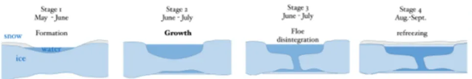
(32) Thèse de Babak Rabbanipour Esfahani, Université de Lille, 2018. 12. 2. 2. Overview on sea ice melt ponds in the Arctic. opment of open water areas, which then again enhance the ice-albedo feedback [9]. A trend to an earlier melt onset and a later freeze-up date in the entire Arctic region for the last three decades is described in literature [10]. The resulting longer melting periods are again a positive factor to the ice-albedo feedback mechanism. Starting in April in sub-Arctic regions, dry snow wettens and begins to melt. Snow grains2 transform and grain size generally increases [11]. Even these first melting processes can reduce the albedo of snowy surfaces by about 10 ∼ 20%. Snow melting processes depend on the properties of the snow cover, mainly on the snow depth. The variability of Arctic snow cover depth ranges from none to several meters in leeward sides of ridges or other obstacles. In the Central Arctic, snow cover usually disappears by the end of June [12]. Melt water of snow and ice accumulates in surface depressions and other surface deformation features. Compared to the much more irregular surface topography of multi-year ice; plane and flat surfaces of first-year ice have the potential to host large and extended melt pond areas [12, 13]. They can reach a coverage of over 50% of the total sea ice area [11]. On a flat topography of first-year level ice and in an early melt stage; the melt pond fraction can even rise up to 90% [14]. As melting develops, pond water drains through porous ice and cracks [15]. The pond properties and distribution on multi-year ice are described as smaller, deeper, and more numerous than on first-year ice [16]. The heat transfer due to convection in water exceeds the one of ice. Additionally, the lower albedo of ponded ice allows a higher penetration of heat into the ice. Both factors yield to a two to three times higher melt rate beneath ponds compared to the melt rate of bare ice [12]. Hence, the ponds deepen and can even melt through the ice layer. With the increasing depth of the ponds, also the diameter decreases [12]. On the one hand, spectral as well as total albedo of bare ice are fairly constant during the melting period. On the other hand, albedo of ponded ice depends on the pond depth and varies throughout the melting period [4]. Melt ponds are nearly salt free and the density maximum of the ponded water lies well above the freezing point [12]. Consequently, radiative heating favors convection within the pond: due to the density anomalies of water, the warmer water will sink down and thus causes further melting. Convection and mixing of the water is additionally enhanced by wind [15]. In late summer, melt ponds tend to melt down to sea level and drain towards the ocean. Mature ponds are effective traps for the first drifting snow. Through the capillar effect, the water level of the pond rises. Therefore, it is less likely that this particular area will be pond covered in the next melting season [12]. Freeze-up starts in late August or early September, caused by low air temperatures. This results in a decreasing melt pond fraction. A snowfall event after freeze-up will cover the melt ponds, resulting in a higher surface albedo. The process of formation of melt-ponds is summarized in Fig (2.5). The large inter-annual variability of the melt pond coverage can be caused by several factors: year-to-year variations of weather (mainly clouds and radiation), amount of melt water availability from snow, variable surface topography, floe size distribution, 2 Snow grains are a form of precipitation. Snow grains are characterized as very small (< 1mm),. white, opaque grains of ice that are fairly flat or elongated. Unlike snow pellets, snow grains do not bounce or break up on impact.. © 2018 Tous droits réservés.. lilliad.univ-lille.fr.

(33) Thèse de Babak Rabbanipour Esfahani, Université de Lille, 2018. 2.2. Representing ponds in climate models. 13. and their effect on runoff-pattern [12, 17].. 2 Figure 2.5 – Summary of melting and refreezing cycle of melt ponds in Arctic in one snapshot.. 2.2. Representing ponds in climate models In this section, we review most used models introduced over the last two decades. There was no pond parameterization in the early sea-ice thermodynamic models [18, 19]. However, observation of rapid reduction of summer Arctic sea ice suggested dynamic effects of melt ponds in the rate of melting of sea-ice. The models, presented here, are described briefly together with the methods used to model melt ponds. In order to complete the discussion, we conclude by describing strengths and weaknesses of each model. These models are mainly about distribution of melt ponds, and internal dynamics of melt pond has been rarely taken into account. The order of introduction of models is from large-scale models to small-scale ones, and finally the models describing dynamics of single melt pond.. 2.2.1. Large-scale models Taylor and Feltham: Melt pond model Taylor and Feltham [20] introduced a one-dimensional, thermodynamic melt-pond model that is based on two-stream radiation model3 instead of commonly used Beer-Lambert law4 representation of radiative transmission in sea ice. This model is advantageous in that the albedo can be calculated from the optical properties and ice thickness, whereas for Beer’s law formulations, albedo is specified as an external parameter. In the presence of melt ponds, a parameterization is used to simulate the variation of optical properties caused by morphological changes to the sea ice during summer. The governing equation for temperature is based upon the equation describing conservation of heat in a mushy layer. Mushy layers describe binary alloys, and consist of a solid matrix surrounded by its melt. For sea ice the solid matrix is composed of effectively pure ice, and the melt is brine. The melt-pond model is primarily focused on Arctic sea ice, because the forcing data describe Arctic conditions; however, it is also applicable to melt ponds in the Antarctic. 3 Two-stream radiation model allows albedo to be determined from bulk optical properties, and a. parameterization of the summertime evolution of optical properties. 4 The Beer-Lambert law is the linear relationship between absorbance and concentration of an. absorbing species. The general Beer-Lambert law is usually written as A = a(λ)bc, where A is the measured absorbance, a(λ) is a wavelength-dependent absorptivity coefficient, b is the path length, and c is the analyte concentration.. © 2018 Tous droits réservés.. lilliad.univ-lille.fr.

(34) Thèse de Babak Rabbanipour Esfahani, Université de Lille, 2018. 14. 2. Overview on sea ice melt ponds in the Arctic long-wave radiation FLW  T 4. sensible and latent heat. Fsens Flat. short-wave radiation FSW FSW. snow. 2. Refrozen. ice layer. Fluid. melt pond. sea ice (mushy layer). Upwelling and Downwelling Streams. Porous. brine drainage. 2-stream radiation model. ocean heat flux. Figure 2.6 – One-dimensional melt pond-sea ice model of Taylor and Feltham [20]. With some straightforward modifications, the model could also be applied to other geophysical surface melt processes such as surface melting of glaciers. As shown in Fig. 2.6, the model uses a three-layer, two-stream radiation model following Perovich [21], where the layers correspond to the melt pond, underlying sea ice and (where it exists) a layer of refrozen sea ice on top of the melt pond. The two-stream radiation model describes the radiation field in terms of an upwelling and downwelling stream. The advantage of this model is that albedo can be explicitly determined, although it suffers from the assumption that the instantaneous radiation is uniform and scattering is isotropic. However Taylor and Feltham argue that as during summer, there is a high percentage of cloud cover [22], thus the assumption of diffuse incident radiation is approximately valid [21]. For computational convenience this model does not use spectral variation of the solar radiation or vertical variation of the optical properties in each layer, and it parameterizes the optical properties in the presence of melt ponds to obtain more accurate summertime temporal variation of albedo. Using wavelength integrated properties should not significantly affect the qualitative results, since most of the radiative energy in the sea ice is absorbed near the surface and this can be well represented using a single-band model [23]. This model consists of many features; for instance, heat transport within sea ice, melt pond and internal region, and snow layer, and finally drainage of ponds. However, the problem with this model is considering constant rate of melting for ice (in which the solid-liquid interface grows with a constant velocity), and independence of liquid layer height.. © 2018 Tous droits réservés.. lilliad.univ-lille.fr.

(35) Thèse de Babak Rabbanipour Esfahani, Université de Lille, 2018. 2.2. Representing ponds in climate models. 15. Melt ponds evolution coupled with CICE model The Los Alamos CICE5 model is based on sea ice conditions and topology of the surface sea ice and was introduced by Flocco et al [24]. When meltwater forms due to snow and surface ice melt, it runs downhill under the influence of gravity. Thus, the topography of the ice cover plays a crucial role in determining the melt pond cover (e.g., [13, 25, 26]). CICE uses a discretized ice thickness distribution function [27] with five ice categories in the reference configuration. In this model it is assumed that each sea ice thickness category is in hydrostatic equilibrium at the beginning of the melt season, so that the sea ice thickness distribution function can be split into a surface height and basal depth distribution. For melt pond parameterization, the model calculates the position of sea level assuming that the ice in the whole grid cell is rigid and in hydrostatic equilibrium. The principle for meltwater distribution within a given grid cell and time step is, then, to take the volume of meltwater and cover the ice thickness categories in order of increasing surface height [28]. In general, the climatology of the reference CICE simulation with this melt pond scheme is in good agreement with observed ice extent and concentration and in reasonable agreement with observed ice thickness. The largest discrepancies occur in the Fram Strait, where the ice is too thin and drifts too fast, and in the Barents Sea. But these regions are of minor importance for studying the impact of melt ponds. The impact of this melt pond scheme can be understood through comparison with three different melt pond approaches. First, artificially pond area and volume is set to zero. Second, this model applies the CCSM3 (Community Climate System Model [29]) radiation scheme instead of the Delta-Eddington radiation scheme [30]. Melt ponds are not explicitly accounted for, but the albedo is adjusted to observations (e.g., SHEBA experiment [31]) that include ponds. Third, this model applies the semi-empirical Bailey scheme [32] in which pond area and depth are parameterized as a function of the volume of meltwater and the change of meltwater volume as a function of surface temperature [28]. Apart from effectiveness of this model on well predicting the behaviour of Arctic seaice, this model does not deal with physical behaviour of ponds, and therefore, further investigation for understanding the dynamics of ponds is needed.. 2. Lüthje: Modeling sea ice ponds Lüthje et al. [25] developed a mathematical model to help understand the relative importance of melting and drainage processes to the summer evolution of the sea-ice cover. Different topographies, unponded ice melt rates, melt rates beneath melt ponds, vertical drainage rates, and horizontal permeabilities were tested. Despite the simplicity of the model physics, the model is able to quantitatively capture the main features of melt-pond formation, spreading and drainage. 5 The Los Alamos sea ice model (CICE) is the result of an effort to develop a computationally ef-. ficient sea ice component for use in fully coupled, atmosphere-ice-ocean-land global circulation models, and it was originally developed to be compatible with the Parallel Ocean Program (POP). The name CICE is derived from "sea ice" and further information about it can be found at. http://oceans11.lanl.gov/trac/CICE. © 2018 Tous droits réservés.. lilliad.univ-lille.fr.

(36) Thèse de Babak Rabbanipour Esfahani, Université de Lille, 2018. 16. 2. 2. Overview on sea ice melt ponds in the Arctic. The model consists of a volume element containing part of the surface of the seaice cover. The volume element is in the shape of a square prism with horizontal edges parallel to the axes of a Cartesian coordinate system fixed in space. The upper surface of the sea ice is given with respect to a fixed plane (for instance z = 0) and the depth of the layer of meltwater on top of the sea ice is denoted initially. Initially, the surface topography is given together with the depth of the sea ice. The surface of the melt pond will lower after a time interval owing to vertical seepage, and the upper surface of the sea ice will lower owing to melting. The horizontal fluxes of meltwater into or out of the volume element per unit cross-sectional area are measured and used to compute volumetric changes of simulated melt ponds. As vertical seepage occurs more rapidly than horizontal redistribution through the surface layer, in each time step of the numerical calculations, the model apply the horizontal flux of meltwater into, or out of, a grid cell only if there is meltwater left after vertical seepage has taken place. Calculations using their model give new insight into processes important for melt pond development. In particular, topography, vertical seepage rate, and unponded ice melt rate turned out to be the most important unknowns in determining the total summertime surface ablation of sea ice. However, the treatment of meltwater flow was relatively crude and the model does not explicitly treat a snow cover. The role of snow and the importance of hydrodynamic processes to determining melt pond evolution is described by Eicken et al. [13, 15]. On this basis, one can speculate about the typical role of snow in a model of melt pond evolution. In particular, as the snow cover melts before the ice beneath it, the distribution of snow will largely determine the initial source of meltwater at the beginning of the melt season. Since, at this time, the sea ice is relatively cold and therefore relatively impermeable, one would expect lateral spreading of melt ponds to dominate vertical drainage into the underlying ocean. This is especially true of flatter, first-year sea ice as the meltwater is not trapped in depressions. The lateral spread of melt ponds might be expected to lead to enhanced melt at the peak in solar radiation, leading to entire melt through of sea ice in places, draining meltwater from a surrounding catchment area. The net effect of this may well be to reduce total ablation as predicted by this model. Although, this model considers the drainage of melt pond in the process of formation, however, the dynamics of melt pond is not taken into account. Moreover, the model can simulate physical area of order 100 meters which compared to the area of Arctic sea ice is quite small. Continuum model of melt pond evolution This model is chosen to determine a model of the melt pond cover through a consideration of the physical processes that have been observed to determine pond evolution [33]. It make use of the sea ice thickness distribution function of Thorndike et al. [27], which was in use until recently in the latest generation of climate models, for example, HadGEM (the UK climate model), the Community Climate System Model (CCSM) at the US National Center for Atmospheric Research, and the Los Alamos CICE sea ice model component. In the sea ice component of climate models, the thickness distribution function is. © 2018 Tous droits réservés.. lilliad.univ-lille.fr.

(37) Thèse de Babak Rabbanipour Esfahani, Université de Lille, 2018. 2.2. Representing ponds in climate models. 17. discretized, so that the area fractions of a small number of thickness classes are calculated and the evolution equation is solved in stages, using operator decomposition [34]. When solving the thermodynamic part of the evolution equation, the presence of melt ponds on the ice should be taken into account because the melt ponds significantly increase the melting rate of the ice they cover during the melt season and provide a store of latent heat that retards freezing during fall and winter. The basic continuum hypothesis, in this model, is that within the horizontal grid cell of a sea ice model, ice of varying thickness is distributed uniformly, with relative abundance determined by the thickness distribution function. In particular, ice with different surface heights are distributed uniformly with relative abundance. This model uses the surface height distribution function to determine the redistribution of meltwater: at the beginning of a time step in numerical model, meltwater is generated and, at the end of the same time step, this meltwater is distributed so that it first covers ice of lowest surface height, and subsequently covers ice of increasing surface height. The meltwater is distributed such that the pond surface height is the same on all pond-covered surface ice height classes. Since the hypothesis is that sea ice of different surface heights are distributed uniformly over the grid cell, the meltwater does not need to travel far horizontally in order to accumulate on the lower ice surface. One of the drawbacks of this model is the inability to explicitly model horizontal transport of meltwater upon or within sea ice in the model because generally the topography of the ice surface is unknown. For the same reason, this model is unable to distinguish between one large pond or a collection of ponds with the same total area and volume. Another disadvantage of this model is that it does not explicitly treat the heat balance in the model. However, it uses a simple parameterization for the melting rate of ponded ice, with constant surface melting rate for bare ice and constant basal melting rate. These assumptions were made to simplify the calculations and isolate the physics of the pond formation and evolution. Using this model, calculations have revealed that during the early part of the melt season, the pond coverage is dominated by snowmelt and accumulation of water with a positive hydraulic head. However, by about day 10 into the simulation, the ice cover becomes sufficiently porous that the pond surface drains to sea level within a few hours. The model is based on many necessary assumptions. However, the model provides a realistic simulation of the fraction of the ice surface covered melt-ponds and maximum pond depth.. 2. Ising model for melt To address the fundamental problem of the evolution of the melt ponds in polar climate science, this model introduces a two dimensional random field Ising model 6 for melt 6 The Ising model, named after the physicist Ernst Ising, is a mathematical model of ferromag-. netism in statistical mechanics. The model consists of discrete variables that represent magnetic dipole moments of atomic spins that can be in one of two states (+1 or −1). The spins are arranged in a graph, usually a lattice, allowing each spin to interact with its neighbors. The model allows the identification of phase transitions, as a simplified model of reality. The twodimensional square-lattice Ising model is one of the simplest statistical models to show a phase. © 2018 Tous droits réservés.. lilliad.univ-lille.fr.

(38) Thèse de Babak Rabbanipour Esfahani, Université de Lille, 2018. 18. 2. Overview on sea ice melt ponds in the Arctic. 2 Figure 2.7 – Melt ponds as metastable islands of like spins in a random field Ising model.[35]. ponds [35]. The ponds are identified as metastable states [36–38] of the system, where the binary spin variable corresponds to the presence of melt water or ice on the sea ice surface. With only a minimal set of physical parameters, the model predictions agree very closely with observed power law scaling of the pond size distribution [8] and critical length scale where melt ponds undergo a transition in fractal geometry [39]. To describe nontrivial spin clustering at zero temperature, the Hi and/or J i j are chosen as random variables; the resulting models are collectively known as disordered Ising models [40]. In particular, one recovers the classical random field Ising model (RFIM) if the Hi are independent random variables and the J i j = J are constant. At zero temperature, the system is usually assumed to follow Glauber single spin-flip dynamics [41] at each update step, the flip is accepted if H decreases and rejected if H increases. The system eventually converges to a local minimum of H , known as a metastable state. Metastable states are especially relevant to physical systems near phase transitions, including supercooled liquids [42] and atmospheric aerosol particles [43]. For disordered Ising models they have been realized experimentally in, for example, doped manganites [44] and colossal magnetoresistive manganites [45]. Despite their importance, metastable states are not completely understood theoretically [41], with analytical results largely restricted to 1D [46] and many intricate issues remaining in 2D [47]. The key factor controlling melt pond configurations is the pre-melt ice topography, represented by random variables h i . In the spirit of creating order from disorder, these variables are assumed to be independent Gaussian with zero mean and unit variance. The lattice constant a = 0.85m is specified as the length scale above which important spatially correlated fluctuations occur in the power spectrum of sea ice topography. The model uses the following update rule for Glauber dynamics, depending on whether there is a majority among the four neighbors of a chosen site. If a majority exists, the site is updated to align with the majority because of heat diffusion between neighboring sites. Otherwise, a tiebreaker rule is introduced that describes the tendency for water to fill troughs: the chosen site is updated to ice if its pre-melt ice height is positive, and water otherwise; see Fig. 2.7. Note that this update rule does not depend on any parameters other than h i . Minimal models such as the RFIM necessarily have limitations. In particular, the RFIM has a percolation threshold very close to 0.5 at H = 0. This threshold decreases transition.. © 2018 Tous droits réservés.. lilliad.univ-lille.fr.

(39) Thèse de Babak Rabbanipour Esfahani, Université de Lille, 2018. 2.2. Representing ponds in climate models. 19. as H decreases, but likely always exceeds the value for real melt ponds. This discrepancy may be attributed to unresolved processes at smaller scales, and/or the observed pre-melt ice topography being spatially correlated rather than completely random. This can be anticipated that, based on a significant amount of observational data, a detailed scheme for choosing the initial spin configuration and update sequence may be formulated. The interpretation of complex Arctic melt ponds in terms of a simple disordered system may well advance the ability to model the future trajectory of the Arctic sea ice pack, e.g., through parameterizations in global climate models [28].. 2. 2.2.2. Small scale models Single melt pond model Skyllingstad et al. [48] investigate the thermodynamic behaviour of melt ponds using two modeling approaches. First approach addresses the heat budget of a melt pond using a large-eddy simulation (LES) model that can directly simulate the motion of water within a melt pond. Use of the LES model allows to estimate the importance of windforcing and heat transport within the pond. However, because of the high computational cost of LES, they could only examine the heat transport processes over periods of a few hours. In addition, three basic pond configurations were considered in the LES experiments, each designed to test the importance of the pond horizontal area versus perimeter. (Fig. 2.8). Figure 2.8 – Horizontal velocity for 4 − m pond with different configurations. Courtesy of Skyllingstad et al. [48]. To examine longer-term pond behaviour, a less complicated bulk model is developed, which concentrates on the radiative heating within the pond. The bulk model simulates pond growth by treating the pond as well mixed and tracks the width, length, and depth of the pond as a function of time. This method differs from previous bulk models by considering the pond size and applying the pond budget equation with a depth-dependent solar flux. The model provides a useful tool that can bridge the gap between expensive, high-resolution LES and single layer ice models as described by Taylor and Feltham [20]. In both the LES and bulk models, they do not account for fluxes of heat and water from lateral transport through porous ice. These factors require a more complete ice model and surface process model. In their model, they address the uncertainties in modeling melt ponds in quantify-. © 2018 Tous droits réservés.. lilliad.univ-lille.fr.

(40) Thèse de Babak Rabbanipour Esfahani, Université de Lille, 2018. 20. 2. 2. Overview on sea ice melt ponds in the Arctic. ing how solar heat is transferred. To estimate the relative importance of side versus edge melting, they apply an LES model that directly simulates the motion of water throughout the pond and the transport of heat from the pond interior to the bottom and sides. The LES model is based on the filtered nonhydrostatic, Navier-Stokes equations with a subgrid-scale closure provided by Ducros et al. [49]. Pond boundaries are simulated using a volume of fluid approach following Steppler et al. [50] and Adcroft et al. [51]. The equations of motion are defined using an enstrophy conserving scheme following Tripoli [52]. Results from the LES pond model indicate that ponds are very likely to develop wellmixed conditions even when ponds begin with significant stratification. Simulations show that very light winds (2 ∼ 3m/s) are able to move pond water vertically, causing transport of heat throughout the pond system. When stratified with a 4 psu salinity gradient, the model predicts a delay in pond mixing of several hours, but still develops a well-mixed equilibrium state. Well-mixed conditions in ponds suggest that heat will transfer equally to the side and bottom of the pond. For the most part, their experiments support this hypothesis; however, pond shape does limit the movement of water even when well mixed. Simulations with a variety of pond shapes and sizes show that the basic ratio of sidewall area to bottom area, can be used to characterize most ponds. For example, as pond size increases, the bottom area increases in relation to the side area. Consequently, relatively small ponds have a larger lateral growth rate from melting in comparison with large ponds. The drawback of this model is that the experiments performed by the model are only able to give estimates of the pond melting rates and do not address pond evolution forced by water inflow and outflow from the surrounding ice. Clearly, these aspects of pond behaviour are also a key element in controlling the ice-albedo feedback. Moreover, the sizes of experiments are independent of internal dynamics of the simulation, i.e. time independent. In addition, the rate of melting is considered constant and set to that suggested by McPhee et al. [53]. Considering the present model, the necessity of investigating the internal dynamics of melt-pond is undeniable. Therefore, in our model we consider the problem of melting through simulation of complete melting process. Similarly, we consider different aspects, e.g. moving boundary and volumetric bulk heating.. 2.3. Summary and open issues Melt ponds are pools of open water that form on sea ice in the warmer months of spring and summer. The ponds are also found on glacial ice and ice shelves. Ponds of melted water can also develop under the ice. Melt ponds are usually darker than the surrounding ice, and their distribution and size is highly variable. They absorb solar radiation rather than reflecting it as ice does and, thereby, have a significant influence on Earth’s radiation balance. This differential, which had not been scientifically investigated until recently, has a large effect on the rate of ice melting and the extent of ice cover. Through this chapter, we described the mechanism that involves formation of melt ponds. Furthermore, we talked about albedo (a measure for reflectance or optical brightness), and effect of melt ponds in reduction of surface albedo of sea ice, which in advance. © 2018 Tous droits réservés.. lilliad.univ-lille.fr.

(41) Thèse de Babak Rabbanipour Esfahani, Université de Lille, 2018. References. 21. results in absorption of more solar radiation and consequently warmer environment. Several models have been developed over last two decades to simulate the distribution of melt ponds in sea ice, and investigate the mechanism of growth of melt pond at large scale, that we briefly mentioned in this chapter. However, there are several questions that still needed to be answered:. 2. i) What are the processes involved in the dynamics of a melt pond, and how do melt ponds evolve? ii) What is heat flux intensity behaviour with respect to the geometry of melt pond, and how it is linked with the melt rate? iii) How can one characterize the corrugation and morphology of bottom melt pond (ice-water) interface ? iv) How solid liquid interface does interact with internal dynamics of melt pond? v) What effects do other constrains, such as internal heating and moving boundary, have on the rate of melting and total heat budget? In the next part, we try to answer these questions and understand the internal dynamics of melt ponds through the numerical simulation of the melting system. Furthermore, the micro-scale study performed here can be used to parametrize the influence of melt pond in large scale.. References [1] O. I. Mamayev, Temperature-salinity analysis of world ocean waters, Vol. 11 (Elsevier, 2010). [2] T. C. Grenfell and G. A. Maykut, The optical properties of ice and snow in the arctic basin, Journal of Glaciology 18, 445 (1977). [3] D. K. Perovich, The optical properties of sea ice., Tech. Rep. (COLD REGIONS RESEARCH AND ENGINEERING LAB HANOVER NH, 1996). [4] D. Perovich, T. Grenfell, B. Light, and P. Hobbs, Seasonal evolution of the albedo of multiyear arctic sea ice, Journal of Geophysical Research: Oceans 107 (2002). [5] R. E. Brandt, S. G. Warren, A. P. Worby, and T. C. Grenfell, Surface albedo of the antarctic sea ice zone, Journal of Climate 18, 3606 (2005). [6] T. C. Grenfell and D. K. Perovich, Spectral albedos of sea ice and incident solar irradiance in the southern beaufort sea, Journal of Geophysical Research: Oceans 89, 3573 (1984). [7] S. G. Warren, Optical properties of snow, Reviews of Geophysics 20, 67 (1982). [8] D. Perovich, W. Tucker, and K. Ligett, Aerial observations of the evolution of ice surface conditions during summer, Journal of Geophysical Research: Oceans 107 (2002). [9] D. K. Perovich, B. Light, H. Eicken, K. F. Jones, K. Runciman, and S. V. Nghiem, Increasing solar heating of the arctic ocean and adjacent seas, 1979–2005: Attribution and role in the ice-albedo feedback, Geophysical Research Letters 34 (2007).. © 2018 Tous droits réservés.. lilliad.univ-lille.fr.