HAL Id: tel-01253164
https://tel.archives-ouvertes.fr/tel-01253164
Submitted on 11 Jan 2016HAL is a multi-disciplinary open access archive for the deposit and dissemination of sci-entific research documents, whether they are pub-lished or not. The documents may come from teaching and research institutions in France or abroad, or from public or private research centers.
L’archive ouverte pluridisciplinaire HAL, est destinée au dépôt et à la diffusion de documents scientifiques de niveau recherche, publiés ou non, émanant des établissements d’enseignement et de recherche français ou étrangers, des laboratoires publics ou privés.
A statistical and multi-wavelength study of star
formation in galaxies
Corentin Schreiber
To cite this version:
Corentin Schreiber. A statistical and multi-wavelength study of star formation in galaxies. Cosmol-ogy and Extra-Galactic Astrophysics [astro-ph.CO]. Université Paris-Saclay, 2015. English. �NNT : 2015SACLS015�. �tel-01253164�
Contents
Acknowledgments / remerciements 1
1 Introduction 5
1.1 Studying star formation in galaxies: a problem of scales . . . 5
1.2 The main questions . . . 7
1.2.1 Are star formation histories smooth or irregular? . . . 7
1.2.2 Why are some galaxies forming much more stars than others? . . . 10
1.2.3 Does the interstellar dust hide a significant portion of the star formation activity in the Universe? . . . 14
1.2.4 Why do galaxies stop forming stars? . . . 18
2 Summary of the work done in this thesis 25 3 The Main Sequence of star-forming galaxies as seen by Herschel 33 3.1 Introduction . . . 33
3.2 Sample and observations . . . 36
3.2.1 GOODS–North . . . 36
3.2.2 GOODS–South, UDS, & COSMOS CANDELS . . . 37
3.2.3 COSMOS UltraVISTA . . . 38
3.2.4 Photometric redshifts and stellar masses . . . 39
3.2.5 Rest-frame luminosities and star formation rates . . . 40
3.2.6 A mass-complete sample of star-forming galaxies . . . 40
3.2.7 Completeness and mass functions . . . 43
3.3 Deriving statistical properties of star-forming galaxies . . . 45
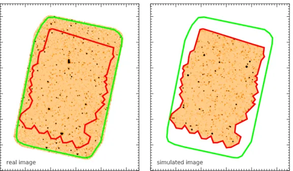
3.3.1 Simulated images . . . 46
3.3.2 The stacking procedure . . . 46
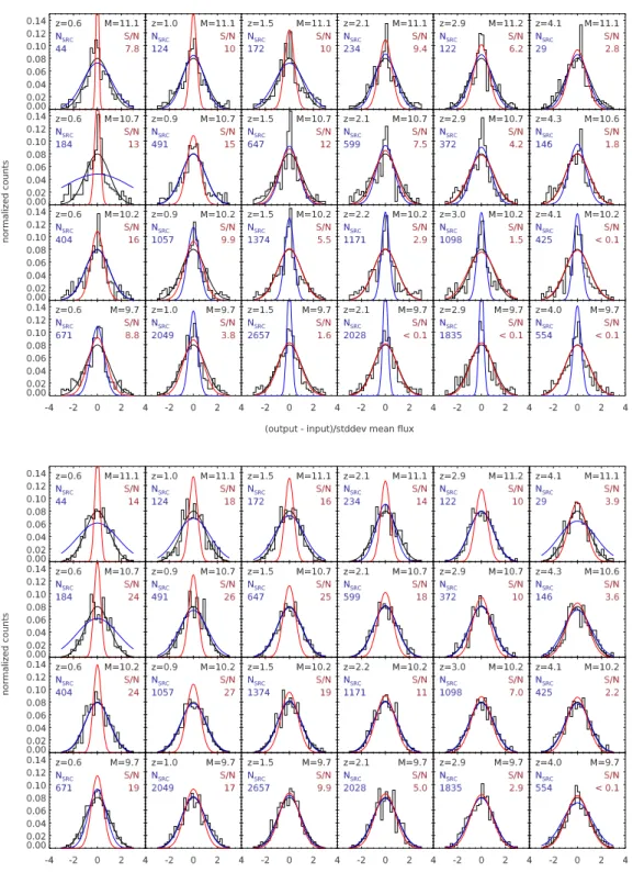
3.3.3 Measuring flux dispersion with scatter stacking . . . 50
3.3.4 SFR dispersion from scatter stacking . . . 52
3.4 Results . . . 53
3.4.1 The SFR of main-sequence galaxies . . . 53
3.4.2 Redshift evolution of the sSFR: the importance of sample selection and dust correction . . . 55
3.4.3 Mass evolution of the SFR and varying slope of the Main Sequence . . 55
3.4.4 Mass evolution of the SFR dispersion around the Main Sequence . . . 56
3.4.5 Contribution of the Main Sequence to the cosmic SFR density . . . 59
3.4.6 Quantification of the role of starburst galaxies and the surprising ab-sence of evolution of the population . . . 59
3.5 Discussion . . . 65
3.5.1 Connection of the main-sequence dispersion with feedback processes . 65 3.5.2 Connection between starbursts and mergers . . . 65
3.6 Conclusions . . . 66
3.8 Appendix: Tests of our methods on simulated images . . . 67
3.8.1 Mean and median stacked fluxes . . . 69
3.8.2 Clustering correction . . . 71
3.8.3 Error estimates . . . 72
4 Modelling the integrated IR photometry of star-forming galaxies 77 4.1 Introduction . . . 77
4.2 A new far infrared template library . . . 78
4.2.1 Calibration on stacked photometry . . . 81
4.2.2 Calibration on individual detections . . . 82
4.3 On the redshift and stellar-mass dependence of fPAH . . . 84
4.4 Appendix: Recipe for optimal FIR SED fitting . . . 85
5 gencat: an empirical simulation of the observable Universe 87 5.1 Introduction . . . 87
5.2 Sample description . . . 88
5.2.1 Multi-wavelength photometry . . . 88
5.2.2 Redshifts and stellar masses . . . 88
5.3 Stellar properties . . . 89
5.3.1 Redshift and stellar mass . . . 89
5.3.2 Star formation rate and obscuration . . . 91
5.3.3 Optical morphology . . . 92
5.3.4 Optical spectral energy distribution . . . 94
5.3.5 Sky position . . . 96
5.4 Dust properties . . . 98
5.5 Generating a light cone . . . 99
5.6 Results . . . 99
5.6.1 Comparison to the observed GOODS–South field . . . 99
5.6.2 Comparison to the measured cosmic backgrounds . . . 102
5.7 Appendix: Efficiency of monochromatic FIR measurements . . . 103
6 The downfall of massive star-forming galaxies during the last 10 Gyr 107 6.1 Introduction . . . 108
6.2 Sample selection and galaxy properties . . . 110
6.2.1 Multi-wavelength photometry . . . 110
6.2.2 Redshifts, stellar masses and star formation rates . . . 111
6.2.3 CANDELS sample for the gas mass measurements at z = 1 . . . 111
6.2.4 HRS sample for the gas mass measurements in the Local Universe . . 112
6.2.5 CANDELS sample for the morphological decompositions at z = 1 . . . 112
6.2.6 Cleaning the 24 µm catalogs . . . 113
6.3 Measuring disk masses in distant galaxies . . . 115
6.3.1 The bulge to disk decomposition . . . 115
6.3.2 Simulated galaxies . . . 117
6.3.3 Estimating the disk mass . . . 118
6.4 Measuring gas masses . . . 120
6.4.1 Dust masses . . . 120
6.4.2 Gas masses . . . 122
6.5 Results . . . 124
6.5.1 The SFR–Mdiskrelation at z = 1 . . . 124
6.5.2 Gas fraction and star formation efficiency at z = 1 . . . 126
6.5.3 A progressive decrease of the SFE with time . . . 129
6.6 Discussion . . . 130
6.6.2 Identifying the actors that regulate the SFE and the gas content . . . 131
6.7 Conclusions . . . 132
6.8 Appendix: Impact of the UV J selection . . . 133
7 Reaching the distant Universe with ALMA 137 7.1 Introduction . . . 137
7.2 Sample selection . . . 138
7.3 Description of the observations and data . . . 138
7.3.1 Notes on interferometric imaging . . . 138
7.3.2 General properties of our data . . . 140
7.4 Data reduction . . . 142
7.5 Flux measurement and detection rate . . . 143
7.6 The z = 4 Main Sequence . . . 145
7.6.1 Calibration of the SFR . . . 145
7.6.2 The SFR–M∗relation . . . 147
7.7 Other galaxies in the field of view . . . 149
7.8 A massive z = 3 galaxy hidden behind a bright star . . . 149
7.9 Discovery of two new high-redshift dusty galaxies . . . 153
7.9.1 Optical to NIR photometry . . . 153
7.9.2 MIR to FIR photometry . . . 155
7.9.3 A first estimate of their physical properties . . . 156
7.9.4 Measuring the redshift with ALMA . . . 158
7.9.5 Potential scientific outcome . . . 160
8 Conclusions and perspectives 163 9 List of publications 167 Bibliography 169 Index 177 List of abbreviations 179 List of symbols 181 Appendix A phy++: a C++ library for numerical analysis 183 A.1 Introduction . . . 183
A.1.1 A brief overview . . . 183
A.1.2 Why write something new? . . . 183
A.1.3 Why C++? . . . 185
A.1.4 Documentation . . . 186
A.2 Application: pixfit and gfit . . . 186
Appendix B Published and submitted papers 193 The Herschel view of the dominant mode of galaxy growth from z = 4 to the present day . . . 195
Observational evidence of a slow downfall of massive star-forming galaxies during the last 10 Gyr . . . 226
Appendix C Approved observing proposals 245 Unveiling a population of massive, dark ALMA galaxies at z = 6 . . . 247
Acknowledgments / remerciements
Ces trois années de thèse ont été pour moi la source de nombreuses émotions. Tout a commencé le 11 juin 2012 par une joie immense : David, mon directeur de thèse, m’annonce que le sujet de ma thèse sera bel et bien financé. C’est le début d’une aventure... Je rencontre alors Mau-rilio. Lui et David seront mes maîtres Jedi tout au long de ma thèse, et le resteront sans doute bien au-delà. Chacun m’enseignera le métier de chercheur de manière différente et souvent contradictoire, me donnant parfois l’impression d’être un disciple du côté Clair et Obscur de la Force à la fois. Quand l’un prône la rigueur et la patience, l’autre met en valeur la visibilité et l’efficacité. Quand l’un ne jure que par les observations, l’autre fait venir un théoricien. Cette constante opposition me donnera fréquemment la migraine, et me fera rire aussi souvent, mais s’avérera surtout être extrêmement utile et formatrice. David et Maurilio, je pense pouvoir dire aujourd’hui que vous m’avez appris une chose importante : avoir confiance en soi n’implique pas de tout savoir sur tout, mais de savoir que l’on n’a pas plus tort que les autres. Évidemment, je ne parlerai pas des autres choses importantes que vous m’avez fait connaître – le limoncello du plateau, le Baba parisien (qui mérite bien une majuscule), les cannoli de Sicile, la zuppa d’orzo de Sesto, le calamar grillé de Crète, le mezze de Chypre, la cantine de l’ESTEC (heu, non), ... Plutôt, je vais juste vous remercier pour tout ce que vous m’avez apporté, et pour tout ce que l’on a pu partager ensemble. À vous deux, vous étiez le directeur de thèse ultime, je n’aurais sans doute pas pu trouver mieux. Merci de m’avoir donné cette chance !
Mon passage à Saclay a aussi été pour moi l’opportunité de rencontrer un solide groupe de chercheurs, permanents, doctorants et post-doctorants. Que ce soit pour parler de résul-tats scientifiques, de la manière de faire de la recherche, des ragots du labo, de politique, ou encore du dernier Gardiens de la Galaxie, vous m’avez été d’une grande aide à chaque fois que je me suis retrouvé confronté à un mur dans mes recherches, ou simplement quand j’avais un coup de mou. Je veux donc remercier, dans le désordre, Matthieu1, Florent, Kata-rina2, Raphaël3 (Rapha), Marc, Anna, Vera, Koryo, Stéphanie, Jared, Pierre-Alain, Frédéric, Emanuele, Émeric, Hervé, Ronin, Aurélie, Maëlle, Tugdual, François, Min-Young4, Em-manuel5 (Manu), Oriane, Fred, Emin, Xinwen, Tao, Anita, Francesco, Jérémy, Daezhong, Chieh An (Linc), Yu-Yen, Kyle et Laure. Je voudrais remercier tout particulièrement Florent, avec qui j’ai partagé de nombreuses pauses thé, accompagnées chaque fois d’innombrables discussions intéressantes, en particulier sur la ségrégation de masse dans les amas globulaires (tu m’as interdit de le mentionner dans les remerciements de mon premier papier, alors je me rattrape ici). Enfin, je voudrais aussi remercier Tao, avec qui j’ai partagé mon bureau pen-dant l’essentiel de ma thèse (je ne traduirai pas ce passage en anglais, ça te fera un exercice pour améliorer ton français), et qui m’a appris tant de choses à la fois sur l’astrophysique et la culture chinoise. À tous, j’attends avec impatience de vous croiser à nouveau, que ce soit au CEA ou en conférence ; vous me manquez déjà. Je ne pourrais pas terminer avec l’équipe du CEA sans exprimer ma gratitude auprès de Jérôme Rodriguez, Pierre Olivier Lagage, Michel Talvard, Anne de Courchelle et Pascale Delbourgo qui s’assurent (ou se sont assurés) chaque 1Merci pour tout ce que tu m’as appris sur le stacking.
2Je rigole encore de ta blague sur Liszt ! 3Ta balle rebondissante ne me manque pas. 4Je t’entends soupirer d’ici.
année de la qualité de vie des doctorants au sein du CEA.
Ailleurs sur le globe, je veux saluer el caballero del Chile, Roger Leiton, ancien doctorant de David, avec qui j’ai régulièrement collaboré durant ma thèse pour mettre en place des projets d’observation sur les grands télescopes de l’ESO (le VLT et ALMA). On ne s’est malheureuse-ment pas beaucoup croisés, mais c’était chaque fois un grand plaisir. Un peu plus proches de la douce France, Mark Dickinson (Tucson, Arizona, un autre fan de Baba) et Adriano Fontana (Rome, plus grappa que Baba) ont joué un rôle tout aussi important durant ma thèse en écrivant de trop nombreuses lettres de recommandation lorsque j’étais à la recherche d’un post-doc. Pour l’instant (et j’espère que ça durera), je ne peux qu’imaginer à quel point c’est un ex-ercice difficile et non moins pénible, ainsi je voudrais vous remercier sincèrement d’y avoir consacré un peu de votre temps. Adriano est également l’investigateur principal de la collabo-ration Astrodeep, qui regroupe plusieurs équipes de recherche en Italie (Rome), en Angleterre (Édimbourg) et en France (CEA & Strasbourg). Comme David est responsable de la section CEA, nous nous sommes rencontrés plusieurs fois et travaillons sur des projets communs. J’en profite donc pour exprimer mon amitié envers les autres membres actifs de cette collaboration: Sébastien, Jim, Nathan, Victoria, Fernando, Fergus, Konstantina, Emiliano, Marco, Paola, Nico et Ricardo. À très bientôt, à Édimbourg et/ou Sesto !
Mes remerciements vont maintenant aux deux rapporteurs, Alberto Franceschini et Dave Alexander, qui ont eu pour lourde tâche de lire le présent manuscrit et d’en valider la pertinence. J’ai été très touché par vos rapports respectifs (en particulier celui de D. Alexander), et je suis très heureux que mon travail vous ait plu à ce point. Le jour de la soutenance, Guillaume Pineau des Forêts, Véronique Buat et Ivo Labbé ont complété le jury. J’ai été très honoré par votre présence (sans doute aussi un peu intimidé), et je vous remercie tous de vous être déplacés et d’avoir posé un regard critique sur mon travail. Je voudrais également en profiter pour remercier une seconde fois Ivo, qui a sélectionné ma candidature pour travailler avec lui à Leiden (Pays Bas) pendant les trois prochaines années. Une nouvelle page se tourne, et j’ose espérer qu’elle sera aussi pleine d’émotions que la précédente !
À ce stade, je suppose que certain(e)s doivent penser : “L’ingrat! Il m’a oublié!” C’est peut-être vrai. Malheureusement, ma mémoire des prénoms me joue trop souvent des tours, et je suis tristement connu pour ma grande maladresse... Dans le doute, je vous remercie aussi ! En revanche, si vous faites partie de mes amis proches ou de ma famille, alors c’est normal. Je vous fait juste poireauter un peu. Bon. Allez, c’est votre tour.
Ces trois années de thèse et ma dernière année de Master n’auraient pas été les mêmes sans toute la “clique de Massy”6: Astrid7, Cédric8, Hanna9, Harold10, Laetitia11, Lucien12, Mathias, Nicolas, Pierre13, Pierre14 et Thomas15. Nos parties de tarot infinies me man-quent cruellement ! Je rajouterai aussi à la liste les contributeurs irréguliers qu’ont été Benoît, Matthieu16, Pierre17et Yunfeng.
Malheureusement, mon temps libre était finalement plutôt limité, et je ne suis pas revenu dans le pays Nantais aussi souvent que je l’aurais voulu. Il n’empêche, les rares fois où j’ai pu vous voir, j’ai été très ému de rencontrer Audray, Emma & Romain, Maël, ainsi que Méla 6À ce jour, plus personne n’habite là-bas, la moitié vit à l’étranger, mais Massy restera toujours l’épicentre de notre
mouvement.
7Ma dulcinée.
8Il y a les gens, et il y a lui.
9Qui m’aura fait connaître l’alcool de sapin et les karjalanpiirakka (Google m’a un peu aidé). 10Chevalier Jésus à ses heures perdues.
11Dont j’ai, pour une fois, bien orthographié le prénom. 12Le gauchiste <3. Tu t’y attendais.
13Strange. 14Charm.
15Qui aura essayé, avec beaucoup de courage mais moins de succès, de m’enseigner la culture de la musique
classique.
16Ooooh. Aaaah. 17Beauty ?
& Ben. Ludo et Audrey m’ont fait le plaisir de venir habiter sur Paris, ce qui a rendu les choses plus simples. Par contre j’ai toujours raté Guilhem (aka. les ch’veux), et je m’en veux. Le temps est loin, maintenant, où on effectuait des missions tard le soir (aux heures paires, toujours), et je repense à tout ça avec beaucoup de nostalgie. Vous m’avez appris à déconner, et il se trouve que c’est une aptitude très utile quand on fait de la recherche (surtout quand on travaille avec David). J’espère tous vous revoir bientôt.
De manière un peu plus régulière, et surtout pour le nouvel an, j’ai pu rendre visite à Romain, Rémi, Anne, Guillaume et Benjamin. Que de souvenirs de chaise qui roule et de trou normand. Que de bon films vus ensemble, et que de navets aussi. Pendant tant d’années vous êtes restés une constante dans ma vie, Romain sans doute plus que les autres vu que je te connais depuis près de quinze ans (ne sois donc pas jaloux Rémi). Merci à vous d’avoir été là. Oh je n’ai pas mentionné tout le monde, et pourtant vous le mériteriez sûrement. Peut-être que je n’ai pas pu vous voir durant les dernières années, mais je voulais tout de même dire un mot de gentillesse aux individus suivants. Vous avez tous un peu contribué à faire de moi qui je suis aujourd’hui. Dans le désordre le plus total, merci à Marco A., Alexis C., Benjamin P., Quentin G., Florian G., Antoine C., Zacharie N., Fabien B., Hugo S., Fred B., un autre Fred B. et sa Mathilde R., Kévin G., Thomas M., Tim C., Arnaud P., Onethenk B., Amaury L., Virginie T., Sylvain B., Justine D., Alexandre R., Sarah G., Thomas F., Rachel K., Annabelle P., Sylvestre P., David E. et Sylvain S. Et merci aussi à Mylène.
On garde toujours le meilleur pour la fin, paraît-il. Il ne me reste plus qu’à remercier ceux qui me sont les plus proches et sans qui je ne serais rien : ma famille. Pour faire honneur aux anciens, je vais commencer par mes deux grands mères, Élise et Françoise. Vous avez toujours su donner de votre amour de façon inconditionnelle à vos petits enfants, quand bien même, dans ces deux familles, exprimer son affection n’est pas une tâche aisée. Ç’a toujours été pour moi un grand plaisir de venir vous voir, et ça le restera. Françoise, ta visite surprise le jour de ma soutenance m’a énormément touché. À toutes deux, votre gentillesse et votre sagesse me guideront tout au long de ma vie. Merci. Viennent alors mes grands pères. Malheureusement, vous aviez déjà quitté ce monde avant le début de ma thèse. La peine est ancienne, mais votre absence reste aujourd’hui gravée en filigrane dans mon esprit. À Henry et Maurice, je dédie ce manuscrit.
Sur une note plus légère, je voudrais maintenant remercier mes oncles et tantes : Laurence & Éric, Alain, Éric R., Christine, Myriam, Mary & René, Philippe & Catherine, Thierry & Catherine, Étienne & Pascale, Valérie & Gérard. C’est toujours avec bonheur que je vous revois pendant les réunions de famille, et je pense avoir eu beaucoup de chance de vous connaître tous et de faire partie d’une famille si vaste. Durant ma jeunesse, vous avez été comme de seconds pères et mères, m’influençant chacun à votre manière, et l’homme que je suis aujourd’hui est le produit de toutes ces interactions. Aujourd’hui je peux voir le monde sous tant d’angles différents grâce à vous. Je voudrais au passage remercier tout particulièrement Myriam qui m’aura nourri et logé sur Paris durant mes deux années de Master, et également Christine pour avoir organisé tant de vacances d’été ! Bien sûr, qui dit oncles et tantes dit cousins et cousines. À vous aussi je voudrais dire merci: Théo, Éliott, Adrien, Noëllie (son Matthieu et la petite Louane !), Jean, Vincent, Lucien, Marine, Romain, Marion et Pauline. Là, mes remerciements vont d’abord aux plus anciens, Adrien et Noëllie, qui ont été des modèles durant toute ma jeunesse18. À Adrien, encore, pour tout le temps qu’on a passé ensemble à jouer, à bronzer, à surfer, à découvrir le monde et les filles.
J’en arrive à la fin. Nicolas, papa, Nathalie, maman, Morgane, sœur. Merci. Vous savez pourquoi. Je vous aime.
Leiden, le 15/10/2015 Corentin 18Mais plus maintenant, je suis un grand !
Chapter 1
Introduction
1.1
Studying star formation in galaxies: a problem of scales
When I first met David, a couple of months before I started working on this thesis, I was sur-prised to see how little is presently known about how galaxies and stars are born, evolve, and then fade away. My field of expertise at that time was theoretical physics (quantum mechanics, general relativity, quantum gravity) and to me it felt natural that progress in these sub-branches of physics has always been slow. Indeed, these are pioneering theoretical works, often address-ing questions that are hard, if not impossible, to connect to the observable world. Extra-galactic astrophysics, on the other hand, deals with objects that, however complex in their structure, are composed of well known elementary bricks: galaxies are made of dust, gas and stars, and each of these components is itself composed of different kinds of atoms, in different proportions and different thermodynamical states. We know how these atoms interact with each other through gravity, electromagnetism, and even quantum mechanics and general relativity, when they mat-ter. Furthermore, these systems are easy to observe: galaxies are found everywhere in the sky, and they evolve on time scales large enough that we can in principle observe even the most distant and faint ones, should we invest enough telescope time. How comes, then, that there are still so many unanswered questions?
I soon realized how wrong my perspective was.
First, this naive picture already starts to break apart if we consider what modern cosmology brings to the game: dark matter and dark energy. While the impact of the latter on individ-ual galaxies is probably negligible, it is nowadays thought that all galaxies live in dark matter “halos” (Blumenthal et al.1984). These are the descendants of the quantum fluctuations that were amplified during the inflation (Press & Schechter 1974; Peebles 1982), and whose im-print can be seen today on the cosmic microwave background (CMB). The nature of this dark matter, let alone its very existence (e.g., Milgrom1983), is a matter of debate. However, it is generally assumed that these exotic particles, whatever they are, only interact with ordinary (or “baryonic”) matter, i.e., what you and I are made of, through gravity. Since the standard model of cosmology predicts that about 84% of the mass in the Universe is made of this dark mat-ter (e.g., Planck Collaboration et al. 2013), this invisible component is expected to dominate completely the gravitational potential at the largest scales, i.e., above tens of kiloparsecs (kpc) where baryonic processes (e.g., hydrodynamics of the gas, stellar winds, etc.) play little role. For this reason, most people believe that it is the dark matter that shapes the large-scale struc-tures, the so-called “cosmological context” in which the individual galaxies evolve. The best example of this is probably the web-like structure that was found in the spatial distribution of galaxies around our Milky Way (e.g., Peacock et al.2001). This dark matter can be of crucial importance, since the accretion of dark matter halos and the baryonic matter they contain can provide a regular flow of cold gas onto a galaxy, replenishing its gas reservoirs and allowing it to sustain relatively high levels of star formation activity over long periods of time (Dekel et al.
Second, even if we knew that dark matter existed and if we understood all its properties, it would still be a challenge to predict accurately the birth and evolution of a whole galaxy. Indeed, and contrary to theoretical physics, the complexity of the problem does not arise from unknown interactions, or unknown constituents: it is a problem of scales. It is easy to forget this fact, especially since we all work with logarithmic units, but studying galaxy evolution requires dealing with scales that span more than ten orders of magnitude (e.g., going from a star to a galaxy1). At the time of writing, the best numerical simulations attempting to describe a whole galaxy are only able to span about six orders of magnitude in spacial scales, reaching a resolution of about 0.1 pc (e.g., Renaud et al.2013). Below this minimum scale, “sub-grid” recipes are used to emulate the complex physics that is supposed to take place: cooling the gas by interaction with dust grains, then collapsing this gas to form new stars, generating stellar winds, and eventually creating super-novae. On the other hand, other numerical simulations can tackle the aforementioned processes by using better resolution in smaller volumes, but then they lack the global context of the whole galaxy, i.e., the gas flows and the associated turbulence coming from the larger scales.
Third, scales are also a problem observationally. Not so much spatial scales as time scales. It is very convenient that galaxies evolve on long time scales, typically of the order of millions of years, because we can re-observe the same region of the sky in intervals of several years with different instruments, and still consider that we observe the same system. But this is also a huge issue: once we observe a galaxy in a given state, we can predict what its future could be, but we will never be able to see this future and confirm our prediction. Or at least not in a human lifetime. It is as if a detective had to solve a crime from a single photograph, shot possibly long after the criminal was gone. While that can be an interesting source of inspiration, it is not scientifically pertinent to ask ourselves what will become of a particular galaxy, because that is not an observable. The only way we can constrain the evolution of galaxies is therefore by studying populations of objects, and establish probable causality links. Thanks to the fact that the speed of light is finite, we can also observe the Universe at various epochs and link together populations of galaxies in terms of progenitors and descendants. We can also make the link between two properties of a given galaxy population, for example the star formation rate as a function of the stellar mass, and use models to see what we can learn from these observed relations. All of our work is therefore based on such statistical arguments.
A philosophical inconvenience emerging from this issue of scales is that we cannot make experimentsin the scientific sense. We cannot “take” two galaxies and make them collide to see what happens. Or capture a galaxy and compress it to see if it suddenly forms more stars. Worse, we only have one Universe to study. If one day we observe the whole sky, and probe the entirety of the observable Universe, we will probably be able to find several complex enough models that will reproduce all these observations2. Having no additional data to rule them out, we will not be able to learn anything more. Fortunately, this is not going to happen any time soon. But still, strictly speaking, and much like cosmology, it can be argued that extra-galactic astrophysics is not a science.
Does it mean that it is not worth spending time and money on these issues? Of course not. In a way, astrophysics is very close to archeology, in that we try to understand our past from what we see today. The fact that we cannot really manipulate or reproduce anything does not prevent us from learning much about how our Galaxy and our world came to be. And it goes even beyond this: it is through astrophysical observations that we have made among the most exciting breakthroughs of the last century. Not only by confirming the predictions of theories, with the existence of super massive black holes or gravitational lenses, but also with 1One could push as far down in scales as the size of a dust grain, a fraction of microns, and up to the size of a galaxy
cluster, a couple of mega-parsecs (Mpc), to span about thirty orders of magnitude. Fortunately, not all these scales are coupled, so it is possible to study them separately to some extent.
2Much like there is always an infinity of functions that fit exactly to a finite number of points. Or much like, and
this is an intended pun to my particle physicist friends, we can always explain any observations at the LHC by adding new particles to the standard model of particle physics.
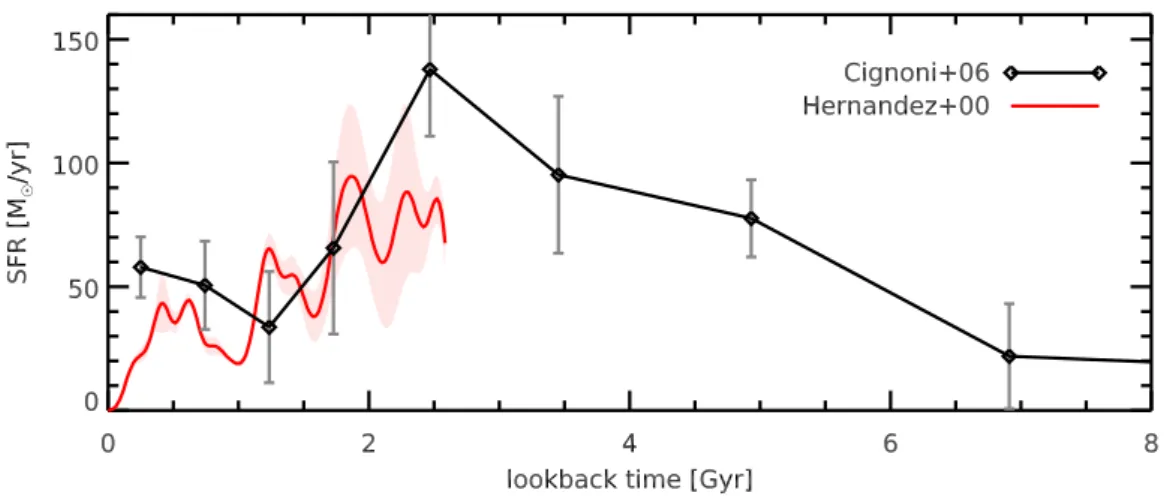
Figure 1.1 – Estimated star formation history (SFH) of the Milky Way (MW). On the y axis is the MW’s star formation rate (SFR), in units of solar masses per year (M⊙/yr), and on the x axis is the lookback time in bilion years, i.e., today is on the left, and the Big Bang is on the right of the plot. The black solid line shows data from Cignoni et al. (2006), which cover a large time window with a poor resolution, and the red line comes from Hernandez et al. (2000), which focus on the last 3 Gyr with a significantly higher time resolution. Both data sets were published in arbitrary units, and are here renormalized to a common reference. The SFH of Cignoni et al. (2006) is rescaled so that integrating it over time yields a total stellar mass of 6.1 × 10¹¹M
⊙(Flynn et al.2006), assuming no mass loss and no merger. The data of Hernandez et al. (2000) are rescaled so that the integral over time between 0 and 3 Gyr matches that of Cignoni et al. (2006). This simple approach is roughly consistent with the MW’s present-day SFR of 4 M⊙/yr, as measured by Diehl et al. (2006).
completely unexpected discoveries, for example with the cosmic microwave background, the expansion of the Universe, or the need for dark matter, dark energy and/or modified gravity. Astrophysics allows us to look at ourselves in a wider context, with a broader perspective. It brings ingredients to physics that, without looking up at the sky, we would have never thought about.
These are the reasons that motivated me during the last three years, and that, hopefully, will keep on amazing me for the years to come.
1.2
The main questions
In this section, I introduce the specific questions I address in this thesis, what we have learned from previous studies, and what they left as unknown. I intentionally do not reveal my own results here, and instead describe the state of the art as it was before the work I have done in Saclay was published. Since this is not an epistemological study, I will not attempt to follow a chronologically rigorous path, nor to report all the previous dead ends that were explored and later abandoned. In the process, I will overlook a number of studies and be unfair to many researchers, all for the sake of clarity. For this, I hope they will accept my apologies.
1.2.1 Are star formation histories smooth or irregular?
One of the major goals of our field is to learn about the star formation history (SFH) of galaxies, or, in other words, the variations over time of the star formation rate (SFR), the rate at which each galaxy is forming new stars.
For example, it is known from detailed study of the properties of stars in our neighborhood that the Milky Way has experienced frequent variations of its star formation rate in the past, about every 500 Myr (Hernandez et al. 2000). These “bursts” seem to happen on top of a
slowly varying, continuous activity that showed a peak about 3 Gyr ago (Cignoni et al.2006), as shown in Fig.1.1. One can also refer to the review of Wyse (2009) for further details. The mechanisms that shape this SFH are still poorly understood today. The regular bursts could be associated with merging events, i.e., the accretion of other smaller galaxies (“dwarf” satellites) on our Milky Way. Not only will these galaxies bring additional stars, they will also briefly destabilize the gas of the Galactic disk and allow it to collapse and form stars more efficiently (this process is discussed further in Section1.2.2). Another explanation which is put forward in Hernandez et al. (2000) is that, since this SFH is estimated from the solar neighborhood only, i.e., a relatively small region compared to the whole Milky Way, these bursts could correspond to the regular passage of the spiral arms. Somewhat surprisingly, the spiral arms are nothing but density waves inside the disk: they are not representative of the motion of individual stars, but emergent patterns caused by different orbits around the Galactic center (Lindblad 1960). When this density wave reaches a given region of the disk, it creates local variations of the gravitational potential and also destabilizes the gas, perhaps in a less efficient way than mergers. This means that, if we were to estimate the SFH from a larger sample of stars not limited to the solar neighborhood (something that Gaïa will soon provide), these variations would vanish, and the SFH of the whole Galaxy would appear much smoother. However, a feature that is expected to remain would be the larger peak that happened 3 Gyr ago. This enhancement of star formation may instead be caused by a major merger, the collision of the Milky Way with another galaxy of similar mass, or by a more intense flow of gas coming from the intergalactic medium (IGM), through a process called “infall” (see, e.g., the discussion in Kennicutt1983). Indeed, our Galaxy must have received large quantities of gas from outside in its past, and probably does so even today. Its present-day star formation rate is currently estimated around SFR = 4 M⊙/yr (Diehl et al.2006), while the mass of gas available to form stars is of the order of Mgas = 2 × 10⁹M⊙ (van den Bergh 1999). Therefore, at this rate the Milky Way would consume all its gas within 500 Myr (see van den Bergh 1957, where this problem was first reported). This latter quantity is known as the depletion timescale, tdep. Such short timescale is not specific to the Milky Way: except for a few exceptions which are not representative of star-forming galaxies (e.g., M31 with tdep = 5 Gyr, Pflamm-Altenburg & Kroupa 2009), the depletion timescales in the majority of galaxies is typically no more than 1 Gyr (see, e.g., Saintonge et al. 2011). This is probably the best evidence that galaxies routinely receive gas from the intergalactic medium.
The question is then, how do galaxies actually consume this gas? Is it mainly through merger events, with episodes of intense triggered star formation? Or rather in a more peaceful but steady way, similar to the density waves created by the spiral arms in the disk? While both channels are known to generate star formation in all galaxies, it remains uncertain today which one typically dominates the star formation histories of galaxies. Ideally, one would transpose the studies described above from the Milky Way to other galaxies, and build a statistically meaningful sample. However, this kind of analysis requires counting individual stars, and that is something we can only do in our closest environment for a handful of galaxies, using the Hubble Space Telescope(HST ).
A key element to answer this question was brought forward by the observation of large samples of galaxies for which we could obtain good estimates of the current SFR and the stellar mass (M∗), both today (Brinchmann et al.2004) and at earlier epochs in the history of the Universe, e.g., 8 Gyr ago (Noeske et al.2007; Elbaz et al.2007). These observations aimed at studying the correlation between the SFR and the stellar mass. The connection with star formation histories becomes obvious once we consider that the stellar mass is the integral over time of the past star formation history3, Rtnow
0 dt SFR(t), while the SFR is just SFR(tnow). In 3Neglecting, for simplicity, the loss of stellar mass due to the death of stars. Assuming the stellar lifetimes of
Bressan et al. (1993), this is 25–30% of the total mass after 1 Gyr for a typical star formation history, and up to 40% after 10 Gyr for an maximally old galaxy. These numbers were obtained assuming the Salpeter (1955) prescription for the mass distribution of newly born stars (the initial mass function, IMF).
*
Figure 1.2 – The correlation between the star formation rate (SFR) and the stellar mass (M∗) of distant galaxies (z = 1), adapted from Elbaz et al. (2007). This is the so-called Main Se-quence of star-forming galaxies. Points are colored according to the rest-frame (U − B) color of each galaxy, i.e., blue points for blue galaxies, and red points for red galaxies. This color is a proxy for the age of the stars: the redder the galaxy, the older are the stars it contains. Therefore, a red galaxy is supposed to have stopped forming new stars long ago (except if the galaxy con-tains dust, as discussed later in Section
1.2.3), while a blue galaxy must still be actively star-forming. The solid line in-dicates the best-fit power law of blue galaxies, and the dotted lines indicate the dispersion around this trend. fact, the quantity of interest here is the specific star formation rate, which is the amount of star formation rate per unit stellar mass: sSFR ≡ SFR/M∗. If one assumes that, at a given epoch, all galaxies have roughly the same age, then this sSFR is proportional to the birth rate parameter: b ≡ SFR(tnow)/hSFR(t)i (Kennicutt1983), where hSFR(t)i is the average of the past SFR. This parameter can be used to estimate the typical “burstiness” of star formation histories. Indeed, if all galaxies were forming stars at a constant rate, by definition they would have b = 1, and at a given epoch they would all have exactly the same sSFR. If on the other hand the star formation histories are very bursty, then one would expect to see a wide distribution of b (or sSFR).
What was actually observed was a correlation between the SFR and M∗ (in logarithmic space), with more massive galaxies having higher rates of star formation, and most importantly with a relatively low scatter in SFR of about a factor of two at fixed stellar mass. An example is shown in Fig.1.2. Since this scatter actually includes measurement errors, the intrinsic scatter is expected to be even lower. For this reason, this correlation was named the “Main Sequence” of star-forming galaxies (MS): as time goes, galaxies are growing in mass and “climb up” the sequence. Their star formation rate increases, until they stop forming stars and “fall down” (this process of shutting down star formation is discussed later in Section1.2.4). This was a very strong step forward. The fact that, over about half the age of the present-day Universe, we observe variations of SFR of at most a factor of two from one galaxy to another places strong upper limits on the variations of the SFH within individual galaxies. This was immediately understood as a sign that these SFHs may be relatively smooth, and that mergers could only play a minor role in the whole star formation story (see in particular the discussion in the following section).
Since then, numerous studies have attempted to refine the measurement of the Main Se-quence. Indeed, mostly because of the presence of dust, correctly estimating SFRs and stellar masses is not always an easy task depending on what data are available, and these estimates are often subject to systematic biases. In fact, many assumptions have to be made in order to de-rive these quantities, since the only thing we observe is the projected brightness of the galaxy at various wavelengths. It is reasonable to worry that these assumptions may lead to wrong conclusions because they oversimplify the situation; for example the real scatter in sSFR may actually be larger than we think. For this reason, the measurement is regularly revisited with deeper or more varied photometry. In particular, I present in Chapter3 the results I have ob-tained during this PhD, building on the work of Elbaz et al. (2011), and taking advantage of the
deepest Herschel and Hubble data to study the spectra of galaxies from the ultra-violet (UV) to the far-infrared (FIR). In this study, we measure the most accurate stellar masses and SFRs, looking back in time as far back as 12 Gyr ago, where the Universe was barely 1 Gyr old, and probing for the first time such a wide time window in a consistent way across such a wide range of wavelengths.
This is clearly not the end of the story though, because there are many regimes that we could not probe, especially the low-mass dwarf galaxies, or the first billion years of the Universe. This study is also not free of assumptions and biases, but I guess it is fair to say that this was, at the time, the best we could do. Further progress will surely emerge out of the new generation instruments that were recently (or will soon be) deployed: the Atacama Large Millimeter Array (ALMA), the James Webb Space Telescope (JWST), Euclid, ... For example, by observing a region of the sky for only a few minutes, ALMA is able to detect galaxies that are up to ten times fainter than what the deepest surveys Herschel could achieve by observing for about 200 hours4. Taking advantage of this incredible sensitivity, we have created a targeted survey with ALMA to study in more depth the young Universe. The data were received in early 2015, and are described in Chapter7.
1.2.2 Why are some galaxies forming much more stars than others?
The existence of the Main Sequence does not nullify the impact that galaxy mergers can have on individual galaxies. It is clear that the most extremely star-forming galaxies in our neighbor-hood are actually pairs of merging galaxies (Sanders & Mirabel1996) with very large sSFRs, indicating that they are likely short but intense phases in the lifetime of these galaxies. Indeed, in an isolated galactic disk, star formation is relatively inefficient because the gas in the disk is stabilized by the shear forces created by the differential rotation of the disk, i.e., the fact that the rotation speed is not the same at all radii (Toomre1964). It was shown only recently in nu-merical simulations that mergers trigger additional instability of the gas through compressive tidal forces (see Renaud et al.2014, and Fig.1.3), effectively allowing a substantial fraction of this gas to collapse and form stars in short timescales (several hundreds of Myr).
Within the ΛCDM cosmological paradigm, it is relatively straightforward to predict the rate of such merging events. Since this is a purely gravitational problem, the baryonic physics does not play an important role, and one only needs to care about dark matter which is much simpler to model. For this reason, the predictions arising from numerical simulations or choke-and-blackboard theory should be relatively robust. In fact, the general expectation is that mergers were much more frequent in the past, because the Universe was overall more homogeneous: today, most of the structures that could merge have already done so. For example, Hopkins et al. (2010a) predicts that major mergers (with a mass ratio of at least 1/3) happen on average every 40 Gyr per galaxy today, while this number would go down to every 4 Gyr if we consider the Universe as it was 10 Gyr ago, i.e., ten times more frequently. Similar trends were found in observations: Kartaltepe et al. (2007) reported that the fraction of bright paired galaxies is only 0.8% today, but was closer to 8% about 10 Gyr ago; a similar factor of ten difference. However, linking observed pair fractions with actual merger rates is difficult. While these numbers are corrected for chance projections, without precise velocity measurements it is unknown what fraction of these pairs will actually end up merging. Perhaps even more importantly, one also need to make assumptions on the observability timescale of a merging event. These uncer-tainties are such that a broad range of scenarios were reported in the literature, from strong to almost no evolution of the merger rate (see, e.g., the compilation of Lotz et al. 2011), but always with a tendency for a decrease with time.
The net consequence is that we expect galaxy mergers to have played a more important 4Note that this comparison is slightly unfair, since ALMA has a very limited field of view (about 15′′), and its
efficiency is substantially reduced when it comes to mapping an entire field, which is what Herschel was designed for.
Star formation history
Energy in compressive turbulence
Figure 1.3 – Left: NGC 4038 and 4039, also known as the Antennae galaxies, an on-going major merger. Both are seen here in the center of the image, and can barely be distinguished from one another. The extended arc-like features, which inspired the name of this pair of galaxies, are called tidal tails. These are made of gas and stars that were stripped from both galaxies through complex gravitational interactions. Copyright: SSRO, reproduced with permission. Right: Simulated star formation history of the Antennae, adapted from Renaud et al. (2014). This data comes from a full 3D model of the merger, with a maximum spatial resolution of 1.5 pc, including gas and stars (see the description of the simulation in Renaud et al.2015). The evolution of the SFR with time is shown with a solid gray line. The green dotted line shows the energy in compressive turbulence, which is predicted by Renaud et al. (2014) to be the dominant way through which mergers densify the gas and trigger additional star formation. The red line indicates the instant where the simulation matches best the current observed state of the Antennae galaxies.
role in the past. Interestingly, and as was seen in the previous section, it was observed that star formation was also globally more intense at these epochs, by about an order of magnitude. Could this be due to the larger merger rates? While this is a tempting explanation, the observed distributions of sSFRs are incompatible with this hypothesis (in the following I summarize the original discussion from Noeske et al.2007). Assuming mergers play a negligible role today because they are rare, we can consider that the typical sSFR we observe in our neighborhood is that of isolated, non-interacting galaxies. Going back in time, as mergers were more frequent, we expect that some galaxies experience episodes of enhanced star formation, and have higher sSFR, while the rest of the population stays at the low sSFR of isolated galaxies. If mergers are predominantly responsible for the intense star formation activity in the distant Universe, a large number of galaxies should be found in this enhanced state and in the end we should see a double-peaked (or bimodal) distribution of sSFR: one peak created by bursty mergers with high sSFR, and another created by non-interacting galaxies with low sSFR. No such strong bimodality is observed among star-forming galaxies, as all galaxies appear to have the same sSFR within a factor of two (see previous section). Therefore, if mergers have any impact, it must be reasonably small, and in any case they cannot be responsible of setting the global star formation rate density in the Universe.
It is actually within this dispersion of a factor of two in sSFR that we think mergers may play their role. One could imagine that a fraction of the galaxies with sSFRs above the average are actually triggered by mergers. This is a path that was explored in several papers, e.g., Elbaz et al. (2011); Rodighiero et al. (2011); Sargent et al. (2012). In particular in Elbaz et al. (2011), David and his co-authors found that, on average, the galaxies that showed an excess sSFR were also showing a specific signature in their spectra (what they called IR8) that could be interpreted as an increased compactness of their star-forming regions. This compactness, in turn, may be a hint that a major merger event recently happened. Indeed, it is clear at least in the nearby Universe that mergers do generate very compact star-forming regions (e.g., Armus et al.1987; Sanders et al.1988). In the distant Universe, however, this is still a poorly explored territory.
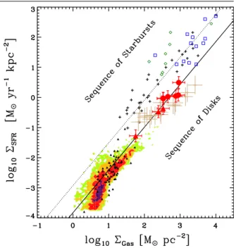
Figure 1.4 – Correlation between the surface density of star formation rate (ΣSFR) and the surface density of hydrogen gas (Σgas), the so-called Schmidt–Kennicutt law, adapted from Daddi et al. (2010a). The red triangles, red circles, brown crosses, black triangles, and the shaded region at the bottom represent “normal” star-forming galaxies at various epochs in the history of the Universe. The black crosses, green diamonds and blue squares are ultra-luminous galaxies, i.e., starburst galaxies (see the original paper for details). The black solid line is the best-fit power law to the normal galaxies, and the black dotted line is this same power law adapted for starbursting systems.
et al. (2011) and Sargent et al. (2012) analyzed the sSFR distributions in a deep Herschel sur-vey, and found that these distributions could be well described by a simple two-component model, dubbed “Two Star Formation Mode” (2SFM, Sargent et al.2012). In this framework, most galaxies are in the “Main Sequence” (MS) mode, with sSFRs varying by a bit less than a factor of two, and a small fraction are in the “Starburst” (SB) mode, with a systematic enhance-ment of their sSFR by about a factor of a few compared to Main Sequence galaxies. In practice, although the philosophy is radically different, this is conceptually very similar to the bimodal sSFR distribution introduced in the previous paragraph (Noeske et al.2007). The main differ-ences are that isolated galaxies and mergers are replaced by the anonymous “Main Sequence” and “Starburst” galaxies, and that these starbursts are a clear minority, both in numbers (3%) and star formation rate density (10%) so that no strong bimodality emerges, consistently with the argument of Noeske et al. (2007).
This finding can be related to another scaling law, namely the Schmidt-Kennicutt (SK) law (Schmidt 1959; Kennicutt 1983), which is one of the most important building block of star formation as we know it. This scaling law tells us that the density of star formation in a given volume is directly connected to the density of hydrogen gas in the same volume5. The correlation is super-linear, meaning that gas is more efficiently converted into stars in denser environments. Recently, it was argued that this scaling law was subject to a bimodal behavior (Daddi et al. 2010a; Genzel et al.2010), with a sequence of “disks” and a sub-population of “starbursts” with greatly enhanced star formation efficiency, see Fig.1.4. Interestingly, these outliers to the SK law are also outliers to the SFR–M∗relation, indicating that they are indeed growing in a different mode, which Daddi et al. (2010a) also suggested to be triggered by major mergers.
Once again, if major mergers are indeed the cause of these starbursts, then the number 5In practice, it is more common in the literature to use surface densities instead of the probably more intuitive
volumedensities. This is actually what was done since the very beginning in the original paper by Schmidt (1959), where he considered star formation inside the disk of the Milky Way. While the disk is actually made of several components, a young thin disk, and an older thick disk, Schmidt assumed that this difference was simply caused by the passing of time, and that all stars were born in a disk of non-evolving width (between 200 and 800 pc, depending on the distance to the center of the Galaxy). For this reason, he averaged his observables along a direction perpendicular to the galactic plane, leading to surface densities of star and gas. Probably by convention, it has remained the standard ever since. When studying distant galaxies, it is questionable whether this choice makes any sense, since only a fraction of these galaxies actually have a clear disk structure (see, e.g., Labbé et al.2003). However, from a more practical point of view, surface densities are model-independent observables, while volume densities cannot be measured without knowing the extent of the object about the third dimension, an information that is often missing and has to be assumed.
of such starbursts should have been larger in the past, where mergers were more frequent. Some studies have already reported such an evolution (e.g., Dressler et al.2009), however it is important to note that these results are very sensitive to the exact definition of a “starburst”. In studies focusing exclusively on the local Universe, it is not uncommon to refer to a galaxy as a starburst if its sSFR (or, worse, its SFR) is larger than a given value. This definition breaks down as soon as one looks back in time, where the SFRs were globally higher, as it would imply that most galaxies in the distant Universe were starbursts. Because it lacks a proper reference point to anchor itself to, this definition is not very useful. An alternative, more interesting definition uses the birth-rate parameter b, introduced in the previous section. One can define a starburst as a galaxy with b > N, i.e., a galaxy whose current SFR is at least N times more than its past average (with, e.g., N = 2 as in Heckman et al. 1990). While more physically motivated, such a definition also suffers from a bias, this time toward young galaxies, or equivalently, toward all galaxies in the young Universe. Indeed, being young, their SFR can only be rising, and their birth-rate parameter must consequently be larger than 1. This does not necessarily mean that they are evolving in a particular way, and for all we know, a young galaxy with b > 1 could be growing like any other young galaxy. Picking a threshold in b high enough should prevent this bias, but this precise threshold depends on the expected star formation history. For example, all star formation histories following the “delayed exponentially declining” functional shape, where SFR(t) ∝ t exp(−t/τ), start with b = 2 and only fall below b = 1 after t >∼ 2 τ, i.e., when the galaxy has already formed more than half of its final mass.
Instead, the definition I will be using in this thesis is the one that allows us to pinpoint unusualbehaviors, galaxies whose star formation rates are different from that of other galax-ies with otherwise similar propertgalax-ies observed at the same epoch in the history of the Universe. One way to achieve this is to define a galaxy as a “starburst” if its SFR is at least N times higher than the average SFR of galaxies of the same stellar mass, at the same epoch. Interestingly, this definition alone does not allow us to disentangle between two different scenarios, correspond-ing to different duty cycles, i.e., the time a given galaxy spends in the starburst mode. First, the enhancement of star formation could be rare, in the sense that it happens only in a few partic-ular galaxies that will always be highly star-forming, while all the others will never experience it in all their lifetime. Second, the enhancement could be more common, but sustained over very short periods of times so that we only see a scant of starbursts at a given instant. Actually, it could very well be both at the same time. A funny picture I have in mind to illustrate this degeneracy is to consider the photograph of a pool filled with frogs, where a handful of these frogs are seen hanging in the air. What could be happening to them? We know that frogs tend to leap quite often, so a natural explanation is that the ones that are hanging in the air were just caught in the act of jumping, and that they will fall down a couple of seconds later. But that’s on Earth. Now, what do you think would happen if instead the photograph was taken on the Moon6? It could very well be that most frogs preferred to stay safe in the water, while a few adventurous ones attempted to jump some time ago and remained hanging above the pool for several (long) hours, lacking sufficient gravity to fall back toward the pool. The fact is, from the picture alone, we cannot tell between these two alternatives. We need to bring additional information, i.e., on which planet the photograph was taken, to figure out what is actually go-ing on. In the case of the starburts, it is the depletion timescale that helps us disentanglgo-ing the different scenarios: as can be seen from Fig.1.4, at fixed gas mass, starbursts are forming stars about ten times faster, therefore their depletion timescales are very low (of the order of 100 Myr, see, e.g., Daddi et al.2010a). For this reason, we know that starbursts cannot remain starbursts for a long time, and unless their reservoirs are quickly replenished with enormous amounts of gas, their star formation activity has to fall down soon after they are observed. This is very well matching the expected behavior of a galaxy experiencing a major merger.
For this reason, in Chapter3(Section3.4.6), I use this definition to study the time evolution 6And if you are willing to assume, for the sake of the argument, that there are pools and frogs on the Moon.
of the starburst population observed in our deep Herschel surveys, and compare it to the trends expected for major mergers to learn more about this extravagant population.
1.2.3 Does the interstellar dust hide a significant portion of the star formation
activity in the Universe?
The first estimate of the SFR density in the Universe was established by measuring the evolu-tion of the UV luminosity of galaxies at different epochs (Lilly et al.1996; Madau et al.1996). Indeed, the sum of the UV light emitted by all the stars in a galaxy is a good tracer of the galaxy’s current star formation rate (e.g., Kennicutt1998b). In star-forming galaxies, the ma-jority of the UV light is produced by very hot stars, which are at least five times more massive and several hundred times more luminous than our Sun. Because of these extreme masses, their gravitational potential is higher, the hydrogen gas they contain is heated to higher tem-peratures and therefore converted faster into helium. For this reason, massive stars have very short lifetimes of less than 100 Myr, compared to the estimated 10 Gyr of our Sun. Knowing this, one can use these stars as a signpost of “recent” star-formation, with a time resolution of about 100 Myr.
There is an issue though. This UV light is made of energetic photons, with wavelengths be-tween 150 and 300 nm. This spatial scale happens to be smaller than the typical size of the dust grainsthat are present in the interstellar medium (ISM, see, e.g., Zubko et al.2004). Therefore, whenever a UV photon intercepts the course of a dust grain, it has a non-negligible probability of being absorbed (or scattered) by this grain, and may never reach our telescope. Depending on the density of dust along the line of sight, only a fraction of the UV light of a galaxy actu-ally manages to escape, and star formation rates can therefore be severely underestimated. An example of such a situation is shown in Fig.1.5.
Fortunately, we know of different ways to recover this missing light. The most direct one is to look for the energy that was absorbed: since energy is always conserved, it has to come out of the dust grain one way or another. In fact, it does so through thermal radiation. When a grain absorbs a UV photon, in virtue of conservation of momentum, the energy it acquires is transmitted in the form of kinetic energy to the individual molecules that compose it. If the grain absorbs such photons at a high enough rate (which is the case for the biggest grains which have the largest cross-section), the grain itself thermalizes and reaches a temperature of a few tens of Kelvins. According to Planck’s law, a black body of such temperature will radiate its energy by emitting photons at wavelengths of the order of 100 µm. This falls in the FIR domain, which is also commonly referred to as the “sub-millimeter” domain (the right hand side of Fig.1.5). Therefore, if one can measure the luminosity of a galaxy in the FIR, and since the dust is transparent to these wavelengths, one can add it back to the observed UV luminosity to recover the intrinsic UV luminosity, and eventually measure an accurate SFR. In most star-forming galaxies, dust attenuation is such that the FIR luminosity is usually much higher than the observed UV luminosity. For this reason, star formation rates obtained this way are usually dubbed “FIR-based”.
The main issue with this approach is that measuring the FIR luminosity is not always easy, and for two reasons. The most important one is that our atmosphere is not transparent between 3 and 800 µm (the atmospheric transmission is poor), precisely because its temperature makes it also radiate at these wavelengths. Some observatories (like JCMT and ALMA) allow us to ob-serve at 300–400 µm, but the observing times needed to detect anything but the brightest nearby objects are usually prohibitive. For this reason, most of what we know of this wavelength do-main comes from space telescopes like Spitzer and Herschel (to name only the two most recent ones), which are obviously not bothered by the atmosphere. However, there comes the second issue: at these wavelengths, the angular resolution is two orders of magnitude worse than in the optical, because of the increased diffraction (which is proportional to the wavelength). This means that most of the distant galaxies observed by Hubble are nothing more than large “blobs”
Figure 1.5 – Spectral energy distribution (SED) of a typical star-forming galaxy similar to our Milky Way. I show here the intensity of the emitted light (in units of L⊙, our Sun’s own luminosity) as a func-tion of wavelength. The blue curve shows how the SED of the galaxy would look like in the absence of interstellar dust, using the Bruzual & Charlot (2003) stellar population models and a constant star formation history. The red curve shows the actual observed SED, where dust absorbs a non-negligible fraction of the stellar light (an attenuation of one magnitude in the V band, i.e., at λ ≃ 0.6 µm). The extinction law is taken from Calzetti et al. (2000), and the dust emission is produced using the models of Galliano et al. (2011).
(a): This sharp decrease of the light intensity at λ ≃ 0.1 µm is called the Lyman break. Photons emitted at wavelengths shorter than this threshold have enough energy to fully ionize hydrogen atoms, regardless of their excitation state. They are therefore very easily absorbed, either within the galaxy, or somewhere along the line of sight in the intergalactic medium (IGM). The net consequence is that we receive essen-tially zero photons shortward of the Lyman break.
(b): This second break in the SED at λ ≃ 0.4 µm is called the Balmer break. This is conceptually identi-cal to the Lyman break, except that this time the photons just have enough energy to ionize an hydrogen atom if this atom is in its first excited state, or above. Because a good fraction of the hydrogen atoms are in their ground state, photons with wavelengths shorter than the Balmer break have a fair chance of not being absorbed. However, the Balmer break is almost coincident in wavelength with another feature, called the 4000 Å break. This break arises in the atmosphere of the stars themselves, and is the result of more complex opacity processes due to non-hydrogen atoms (e.g., calcium).
(c): These prominent features in the mid-infrared between λ = 5 and 15 µm are created by a combi-nation of numerous emission lines which are emitted by large carbonated molecules, called polycyclic aromatic hydrocarbons (PAHs). This is a peculiar type of dust grain typically found within star-forming regions. They are relatively fragile, and tend to be destroyed by too intense radiation fields. Their con-nection to physical processes inside galaxies are still not very well understood.
(d): This is the emission of normal dust grains, re-emitting the stellar light that was absorbed. It is the sum of many gray bodies of different temperatures, ranging between a few tens to a hundred of Kelvins. I show here a typical such combination, but the shape of this part of the spectrum can vary significantly from one galaxy to another, depending on the geometry of the dust clouds and their position relative to young stars, but also on the physical composition of the dust (i.e., silicate versus carbonated grains, and the grain size distribution).
in FIR images: we cannot see their detailed structure, and worse, galaxies appear so big that they tend to overlap, making it difficult (if not sometimes impossible) to robustly attribute the observed flux to the right counterpart. This is called the problem of “confusion”, and is illus-trated in Fig.1.6. The only way to reduce this diffraction is to use larger mirrors7. However, because of practical constraints during launch, the size of the mirror on these space telescopes 7Or, equivalently, to use interferometry, which is very common in the radio domain.
Figure 1.6 – Left: A 30” × 30” region of the cosmological deep field GOODS–South, as observed by Hubbleand shown here in false colors (F606W+F850LP+F160W, i.e., green, red, and near-infrared). These very deep observations allow us to detect many galaxies at varying distances. Right: The same region of the sky observed this time by Spiter (24 µm as blue) and Herschel (100 µm as green, and 160 µm as red). The most obvious detections are pinpointed with white circles, and reported on the Hubble image. These two pictures give an example of the fraction of galaxies for which we have a far-infrared detection.
is much smaller compared to that of their ground-based equivalents. For example, the mirror of Spitzerhas a diameter of only 0.9 m, while that of Herschel, the largest ever launched, is 3.5 m wide. In comparison, the standard mirror size for optical telescopes nowadays is about 8 m, and up to 10 m for the largest ones. Sub-millimeter ground-based telescopes like the JCMT can reach even up to 15 m.
In the end, in a typical cosmological deep-field observed by Hubble, Spitzer and Herschel, we can measure the FIR luminosity of only 15% of the galaxies with stellar mass larger than 3×10⁹M
⊙(see Section3.2.6). The other ones are too faint to be detected in the FIR, even on the deepest Spitzer and Herschel images. There are of course many things to do with these 15%, and the study of these detections has provided a wealth of key results during the past ten years (e.g., Elbaz et al.2007; Magnelli et al.2009; Tacconi et al.2010; Daddi et al.2010a; Rodighiero et al.2011; Elbaz et al.2011; Magdis et al.2012). In this thesis, I present in Chapter3(Section
3.4.6) new results about the evolution of the starburst population (introduced in the previous section) which are only based on this somewhat limited sample. Yet, we would definitely like to be able to measure SFRs for the remaining 85%, since Herschel and Spitzer detections only unveil about half of the star formation rate density of the Universe (see Section 3.4.5), or, equivalently, of the cosmic infrared background (CIRB, e.g., Leiton et al.2015).
This is actually possible by interpreting in a clever way the observed UV spectrum of the galaxy (Calzetti et al.2000). We do not know a priori how bright is the intrinsic spectrum, i.e., what we would see without dust, but we do have a good idea of the shape of this spectrum, in particular its spectral slope β. The spectral slope characterizes the way the light intensity varies with wavelength. A “gray” slope means that the light has the same intensity at all wavelengths, a “blue” slope indicates that the galaxy is brighter in the short wavelengths, while a “red” slope means the opposite8. It turns out that the intrinsic spectral slope of a star-forming galaxy between 0.1 and 0.3 µm is fairly blue (see Fig.1.5). Then, because the strength of the dust absorption depends on the wavelength, the light at the shortest wavelengths will be more 8These names were not chosen randomly: these colors are those that our eyes would perceive with such spectra.
attenuated than the light at the longest wavelengths. In the end, dust will tend to make the observed spectral slope redder (again, see Fig. 1.5). By measuring this observed slope, we can estimate how much dust is present in the line of sight, and recover the intrinsic spectrum. This is informally known as the “β-slope” technique, and by opposition to the FIR-based SFRs introduced above, this method provides “UV-based” SFRs.
Measuring fluxes in the UV domain is much easier than in the FIR. This is especially true for distant galaxies, for which this emission in shifted by the cosmic Doppler effect into the optical domain, which is easily accessible from the ground. Thanks to this fact, we have access to the UV spectrum of essentially all the galaxies detected in cosmological deep fields, allowing us to derive star formation rates even for very faint galaxies. For this reason, UV-based SFR are very commonly used in the literature (e.g., Meurer et al.1999; Steidel et al.1999; Daddi et al.
2004a; González et al.2010; Bouwens et al. 2011, to only cite a few of the most influential works).
The problem of this approach is that it requires quite a number of assumptions. At first sight, the most obvious one is the assumption about the spectral slope of the intrinsic spectrum. While it is true that all star-forming galaxies will have blue intrinsic spectral slopes (because their light is dominated by the young and massive stars), the precise value of the slope will depend on the star formation history of the galaxy: a recent burst will make the slope slightly bluer, while a declining star formation activity will make the slope slightly redder (Leitherer & Heckman1995; see also Boquien et al.2012). Other factors can have similar effects to some extent, like the stellar metallicity Z of the galaxy, which is the proportion of stellar baryons which are neither hydrogen nor helium (i.e., “metals”: oxygen, iron, ...). But probably more problematic are the assumptions about the dust. The transition from the observed to the intrinsic slope is made using an extinction curve, which tells us exactly how efficient is a parcel of dust at absorbing photons as a function of wavelength. Observations of our neighborhood, either within the Milky Way (Witt et al.1984) or peering inside its satellites like the Small Magellanic Cloud (SMC, Prevot et al.1984), have shown that this curve is not universal (see, e.g., Gordon et al.2003). In particular, it is expected to depend on a combination of factors, among which are the distribution of dust grain sizes and their chemical properties. Finally, building the effective extinction curve over the whole galaxy requires assumptions on the geometry of the dust cloud, i.e., how is the dust spatially distributed with respect to the stars. For example, the usual assumption is that the stars are located behind a uniform dust “screen” of variable width. Another very common and similar technique is to use a model to interpret simultaneously the whole spectrum from the UV to the near-infrared (NIR), including the stellar emission and the dust absorption, which is known as “spectral energy distribution (SED) fitting” (see Silva et al.1998; da Cunha et al.2008; Kriek et al.2009; Noll et al.2009, where some of the most commonly used codes are described). While it may help to remove some degeneracies, e.g., with respect to the star formation history or the metallicity, it essentially boils down to the same mechanism to estimate the star formation rates, and therefore requires the same set of assumptions9.
It turns out that, in spite of all these (sometimes crude) assumptions, the end result is on average in good agreement with the more direct estimates obtained from the FIR luminosity of local galaxies (Meurer et al. 1999; Calzetti et al.2000), although some correction were later published (Takeuchi et al.2012). This puzzling agreement probably shows that although each galaxy is unique in its detailed properties and structure, most of the differences are washed out when averaging quantities over the whole volume of the galaxy10. Most, but not all. While these dust corrections appear to be working for the majority of Main Sequence galaxies (e.g., Daddi et al.2007b; Rodighiero et al.2014), a number of studies have shown that these tech-9There are codes which actually interpret the photometry from the UV all the way up to the FIR in a consistent
way, when FIR photometry is available. In this case, the mechanism to estimate the SFR is much closer to the FIR-based approach.